Article

Evaluation of Ensemble Inflow Forecasts for Reservoir Management in Flood Situations

1
Civil Engineering Department, Hydraulics, Water Resources and Environment Division, Faculty of Engineering, University of Porto, Rua Roberto Frias, 4200-465 Porto, Portugal
2
Interdisciplinary Centre of Marine and Environmental Research (CIIMAR), University of Porto, Terminal de Cruzeiros do Porto de Leixões, Avenida General Norton de Matos, 4450-208 Matosinhos, Portugal
*
Author to whom correspondence should be addressed.
Hydrology 2023, 10(2), 28; https://doi.org/10.3390/hydrology10020028
Submission received: 30 November 2022 / Revised: 14 January 2023 / Accepted: 16 January 2023 / Published: 19 January 2023

Abstract

:
This paper describes the process of analysis and verification of ensemble inflow forecasts to the multi-purpose reservoir of Aguieira, located in the Mondego River, in the center of Portugal. This process was performed to select and validate the reference inflows for the management of a reservoir with flood control function. The ensemble inflow forecasts for the next 10-day period were generated forcing a hydrological model with quantitative precipitation forecasts from the High-Resolution Model (HRES) and the Ensemble Prediction System (EPS) of the European Center for Medium-range Weather Forecasts (ECMWF). Due to the uncertainty of the ensemble forecasts, a reference forecast to be considered for operational decisions in the management of reservoirs and to take protection measures from floods was proved necessary. This reference forecast should take into account the close agreement of the various forecasts performed for the same period as also the adjustment to the corresponding observed data. Thus, taking into account the conclusions derived from the evaluation process of the consistency and the quality of the ensemble forecasts, the reference inflow forecast to the Aguieira reservoir was defined by the maximum value of the ensemble in the first 72 h of the forecast period and by the 75th percentile in the following hours (from 72 to 240 h).

1. Introduction

The concept of probabilistic weather forecasting, using Ensemble Prediction Systems (EPS), was introduced in meteorology in the early 1990 s. It has since been increasingly used worldwide in the operational forecasting of future meteorological conditions [1,2,3,4,5,6,7].
Ensemble forecasting techniques are generally based on the analysis of multiple forecasts for the same place and time, thus enabling the incorporation of existing uncertainties into a forecast. Towards this purpose, a numerical method is used to generate a representative sample of possible future states of a dynamical system. In this approach, several numerical forecasts (deterministic predictions) are made using the same model, using slightly different initial conditions, which are established depending on the existing set of records (past and current data). In this way, it is possible to analyze the impact of model uncertainties on forecasts made worldwide [2,3,6,7,8]. Ensemble forecasts can also be built from numerical forecasts obtained by different forecasting models, different formulations of a forecasting model, or even using forecasts from different forecasting centers [2,3,6,7].
Building upon the good results from the use of the EPS in weather forecasting, this approach was gradually applied in other disciplines, namely related to hydrology, as is the case of flood forecasting [3,4,5,6,7,8,9] or of reservoir management [10,11,12,13,14,15]. The growing interest in this matter led to the creation, in 2004, of the HEPEX (Hydrologic Ensemble Prediction Experiment), which is a global community of researchers and users of hydrological ensemble predictions that share their knowledge and experiences in the use of this approach, improving and fostering the use of ensemble hydrological forecasts [3,6,7,9,16,17].
Any prediction system, whether deterministic or probabilistic (by ensemble), is subject to different types of errors. Knowledge of the quality and uncertainty factors underlying the forecasting system is therefore key for the operational use of forecasts to be considered reliable. This is an imperative in flood forecasting, in particular with regard to its use for the management of reservoirs with the function of controlling or minimizing the effects of floods downstream. Operational decisions must be made based on inflow forecasts, which comprise many sources of uncertainty derived from the hydrological modelling process, such as the model’s formulation and parameterization, the model’s initial conditions and the input data, especially the meteorological data [7,11,12,14].
The evaluation of the quality of a forecasting system generally consists in measuring the degree of correspondence between forecasts and real observed values—i.e., to the verification of the forecasts. It can be assessed using many statistical metrics and methods: from simple parameters, such as the simple mean errors, to the analysis of histograms. Some of these methods are applicable to deterministic or ensemble forecasts only, whereas other methods are applicable to both types. In cases where ensemble forecasts are represented by the mean or a percentile of the ensemble distribution, for example, specific methods for deterministic forecasts can also be applied. However, methods that focus especially on ensemble forecasts allow for a better analysis of forecast uncertainty. On the other hand, some methods are applicable to the prediction of discrete events, such as the occurrence or surpassing of a determined threshold for a variable, whilst the others apply only to the prediction of continuous variables. Several authors have described the application of different forecasts’ quality evaluation methods [6,7,11,18,19,20,21,22,23]. An example worth mentioning, since it was used in this study, is the Ensemble Verification System (EVS) [20]—a computer application developed by the NOAA’s National Weather Service. It automatically applies several of the verification methods most often used internationally at the operational level to evaluate ensemble forecasts of continuous numerical variables, such as temperature, precipitation and streamflows.
The results that enable a forecast to be qualified as optimal, according to each type of statistical metric or method of quality evaluation, are presented in the bibliography e.g., [6,7,20,24]. However, no reference criteria were found to classify the quality of forecasts for the full range of possible results from these methods.
Depending on the application of a forecasting system, some quality attributes and their respective evaluation methods are more relevant than others. With regard to the identification of flood situations, the ability to discriminate flood flows is of particular importance, since flood warnings are only effective if they are consistently correct [20,23,25]. On the other hand, for the operational management of a reservoir, it is important that the forecast bias be small so that the flow volumes predicted over time are as close as possible to the observed values [6,7,12].
In addition to quality, a forecasting system can be evaluated according to other perspectives, particularly through the evaluation of: (i) consistency, which is the degree of agreement between forecasts; and (ii) value, defined as the degree of utility of forecasts, either in economic terms, or on the basis of other measurable benefits [7,18,21]. The three characteristics—quality, consistency and value—are closely interconnected and positively correlated, i.e., a forecasting system that reports good results in one of the properties also tends to report good results in the others [6,7,18,25,26].
The present work focused on the evaluation of ensemble inflow forecasts to a multi-purpose reservoir. It intended to assess the degree of reliability that can be expected from the evaluated forecasts, that is, how closely the hydrological forecasts adhere to the observed values in a general way and also in specific cases of occurrence of high flows that can cause flooding situations.
The concept of ensemble forecast implies having a large number of prediction results for the same period. The dispersion and uncertainty of these results require a reference forecast to take operational reservoir management decisions and to enact protection measures from floods. Therefore, the present work was performed with the purpose of selecting a reference forecast for the decision-making process of the management of a reservoir with a flood control function. This reference forecast should take into account relevant statistical parameters, such as the matching approximation of the various forecasts performed for the same period (consistency analysis) and the adherence to the corresponding observed data (verification or quality assessment).

2. Materials and Methods

2.1. Study Case

The present work focuses on inflow forecasts to the multi-purpose reservoir of Aguieira, located in the Mondego River, in the center of Portugal (Figure 1).
With a total storage capacity of 450 hm3, the Aguieira Reservoir is the largest reservoir in the Medium Mondego multi-purpose reservoirs’ system and the one located further upstream on the Mondego River. It holds an important role in streamflow regulation and flood control (in particular, for the protection of the riverside area of the city of Coimbra), in addition to serving other purposes, namely: hydropower generation, irrigation and municipal and industrial water supply. The Aguieira Dam, completed in 1981 and operational since then, makes this possible.
The watershed that drains to the Aguieira Reservoir has an area of 3070 km2, corresponding to approximately 46% of the total area of the Mondego River basin. It is located in the rainiest area of the Mondego basin and includes the inflows of the Dão River, the main tributary of the Mondego River, whose confluence is located immediately upstream of the study section [7,27]. The ground elevation varies approximately from approximately 1990 m, in the Serra da Estrela mountains, where the Mondego River rises from, to approximately 40 m, at the base of the Aguieira dam. The climate in this region is marked by the influence from the Atlantic Ocean, becoming progressively more humid with increasing altitude and in the interior of the basin. The wet season, when most of the year’s precipitation occurs, and the probability of flooding is greatest, occurs from mid-October to mid-April [7].

2.2. Methodology

The data used in this study consisted in daily ensemble streamflow forecasts for the upcoming 10 days’ period to the Aguieira reservoir. These data were obtained with a hydrological model of the Mondego River basin designed for this purpose based on the HEC-HMS software, using the corresponding ensemble precipitation forecasts as meteorological input data. This hydrological model and its calibration and validation processes are described in a paper published by the same authors [27]. As meteorological input data in the model, an ensemble of 52 quantitative precipitation forecasts, with a time-step of 3 h and a forecast horizon of 10 days, were used to obtain each daily inflow forecast. Such precipitation data were derived from the High-Resolution Model (HRES) and the Ensemble Prediction System (EPS) products, provided by the European Centre for Medium-range Weather Forecasts (ECMWF) at 00 UTC of each day [28].
The evaluation process of these ensemble inflow forecasts was carried out for the 4-year period from 1 March 2010 to 28 February 2014 (the period for which the observed inflow data to the Aguieira reservoir were available) and was based on the evaluation of the consistency and the quality of the flow forecasts for each day during that period.
First, a graphical analysis was carried out to evaluate, in a visual and simplified way, the forecasts linked with one of the biggest floods recorded during the period of analysis, which occurred on 30 March 2013. For that purpose, the ensemble inflow forecasts in the 6 days prior to the occurrence of the respective flood peak were analyzed.
Subsequently, a more sustained and comprehensive evaluation was carried out, covering the entire 4-year period and carried out through the metrics and statistical processes indicated below.
The consistency of the forecasts was evaluated by analyzing the matching approximation among the various members of the ensemble forecasts performed on the same day, represented by the dispersion of the ensemble. For this purpose, the standard deviation (STD), for each forecast horizon, was calculated for all performed ensemble forecasts (one per day, during the analysis period).
Considering the purpose of the forecasts under analysis– flood forecasting for the operational management of reservoirs in these situations—an attempt was made to choose a set of metrics and/or statistical processes suited to describing the quality attributes considered most important for this purpose, namely: total error, bias, reliability and discrimination. Given that there are several evaluation methods for each of these attributes that can be employed, only one method per attribute was chosen, with the exception of the evaluation of the total error, for which three statistical measures were considered since they address different types of forecasts (see Table 1). Thus, to evaluate the quality of the forecasts, the following statistical metrics and methods were considered: Mean Absolute Error (MAE), Relative Mean Error (RME), Mean Continuous Rank Probability Score (MCRPS), Brier Score (BS), Rank Histogram (RH) and Relative Operating Characteristic Diagram (ROCD). The selection of these methods was based on recommendations from the literature and results from their use in similar applications [3,11,20]. The description and details of the application of these statistical methods can be found in the references [20,23,24].
The specific evaluation methods for deterministic forecasts—MAE and RME—were applied to the mean of the ensemble distribution.
For the application of the statistical methods, Ensemble Verification System (EVS) software was used [20]. Regarding the methods that are focused on the surpassing of a specific threshold, such as BS, RH and ROCD, two thresholds with interest for the management of the reservoir were considered:
(a)
Threshold 1: 100 m3/s, which corresponds to the mean value of the incoming flow to the reservoir during the wet period (December to March), in the 4-year period of records under analysis;
(b)
Threshold 2: 500 m3/s, which corresponds to the maximum flow capacity of the hydraulic circuit of the dam, with the circuit discharge corresponding to the one to be first used in case of flooding.
These two thresholds were also used in the analysis of the remaining statistical methods mentioned above (MAE, MCRPS and RME), to evaluate the performance of forecasts specifically in scenarios of occurrence of higher inflow values, whilst excluding from the application of these statistical methods the observed inflows with values below the defined thresholds. These methods were then applied to the full data series and to two subsets of data defined through the established thresholds. In any case, when applied using EVS, these methods compare the average of the forecasts with the corresponding observed value, for a given forecasting period.
All the evaluation methods considered were applied with a time step of 3 h and a horizon of 240 h, thus obtaining the corresponding results for each forecast horizon (0–240 h).

3. Results and Discussions

3.1. Graphical Analysis

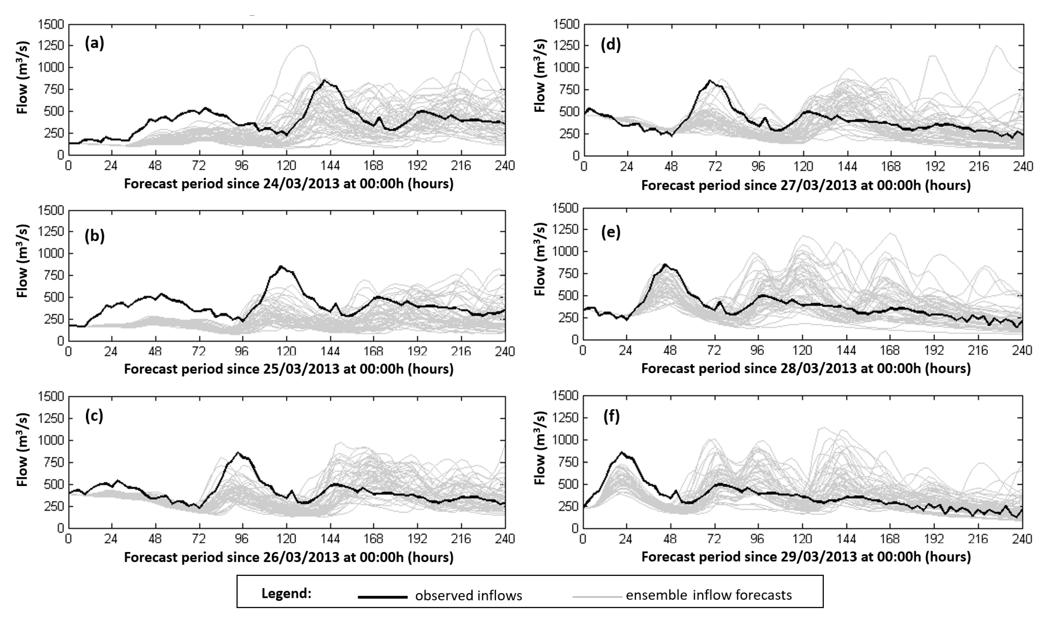
Figure 2 shows the hydrographs of the forecasted and observed inflows to the Aguieira dam, in the 6 days before the flood that occurred on 30 March 2013. In each graph, gray lines represent the various members of the ensemble inflow forecasts, performed in the day stated in the legend of the abscissa axis, for the following 10 days; the black line corresponds to the hydrograph observed in the same period.
Focusing on the degree of dispersion of the ensemble forecast members in the various graphs depicted in Figure 2, in general, dispersion increases with the forecast period. To put it more precisely, it is noticeable that, in most cases, up to a forecast period of 48 to 72 h, the ensemble forecast members report very close values and that from that point onwards, dispersion increases significantly. This simple analysis enables us to infer that forecasts are, in general, more consistent up to a forecasting period of 72 h, and that thereafter they lose consistency.
Turning to the analysis of the quality of the forecasts, by comparing the hydrographs of ensemble inflow forecasts with those actually observed, the following key aspects were evaluated: (i) the ability to predict the occurrence, as well as the value or magnitude, of the flood peak (i.e., the maximum flood flow value) and (ii) the graphical positioning of the observed hydrographs relative to the members of the corresponding ensemble flow forecasts.
In what concerns the first aspect, the occurrence of the flood peak is, in general, predicted at least 6 days in advance. Furthermore, the consistency of this forecast increases as the forecast date approaches the respective day of occurrence. On the other hand, whilst forecasting the magnitude of the flood peak, the same pattern did not hold.
Regarding the position of the observed hydrograph relative to the members of the ensemble forecasts, the scenario that displays a better forecast quality is, by definition, that in which the observed values are within the range of distribution of the ensemble members. It can be inferred from all the graphs shown in Figure 2 that, in effect, this is likelier to happen when the dispersion of the members is greater and consequently the consistency is lower. As is highlighted in the figures below, this happens more frequently for the longer forecast periods, i.e., beyond 72 h.

3.2. Statistical Analysis of the Consistency

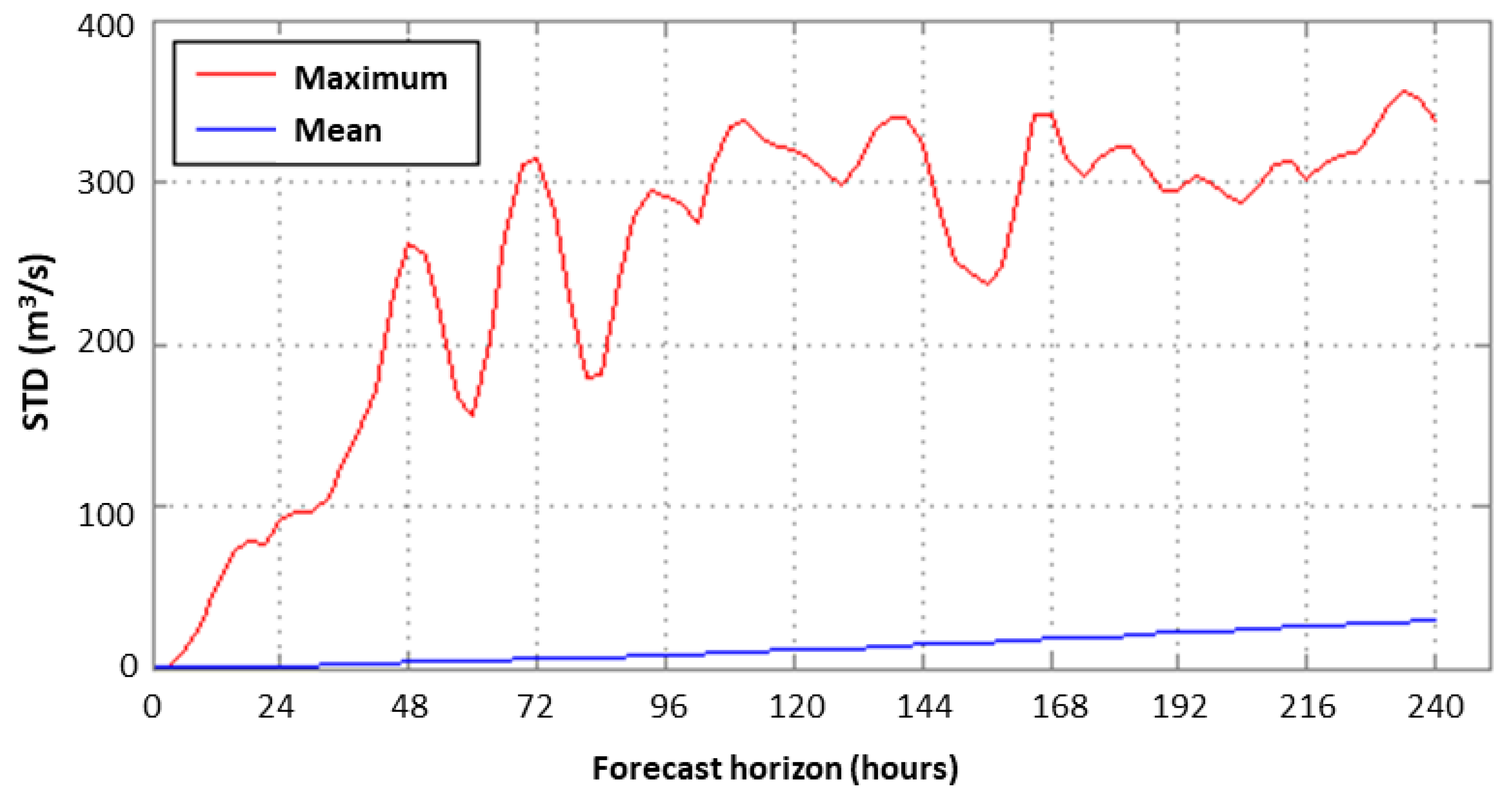
As mentioned, the consistency of the forecasts was assessed by means of the evaluation of the standard deviation, calculated for each forecast horizon, along all the ensemble forecasts performed in the 4-year period of analysis. Figure 3 shows the mean and maximum values of the standard deviations obtained for each forecast horizon. Those results allow us to characterize the dispersion of the ensemble members over the forecast horizon. As can be observed, the standard deviation increases with the forecast horizon (for both the mean and the maximum STD values), which means that the dispersion of ensemble members also increases.

3.3. Statistical Analysis of the Quality

The results obtained with the application of the statistical methods used in the evaluation of the quality of the forecasts are presented below, in the Section 3.3.1, Section 3.3.2, Section 3.3.3, Section 3.3.4, Section 3.3.5 and Section 3.3.6.
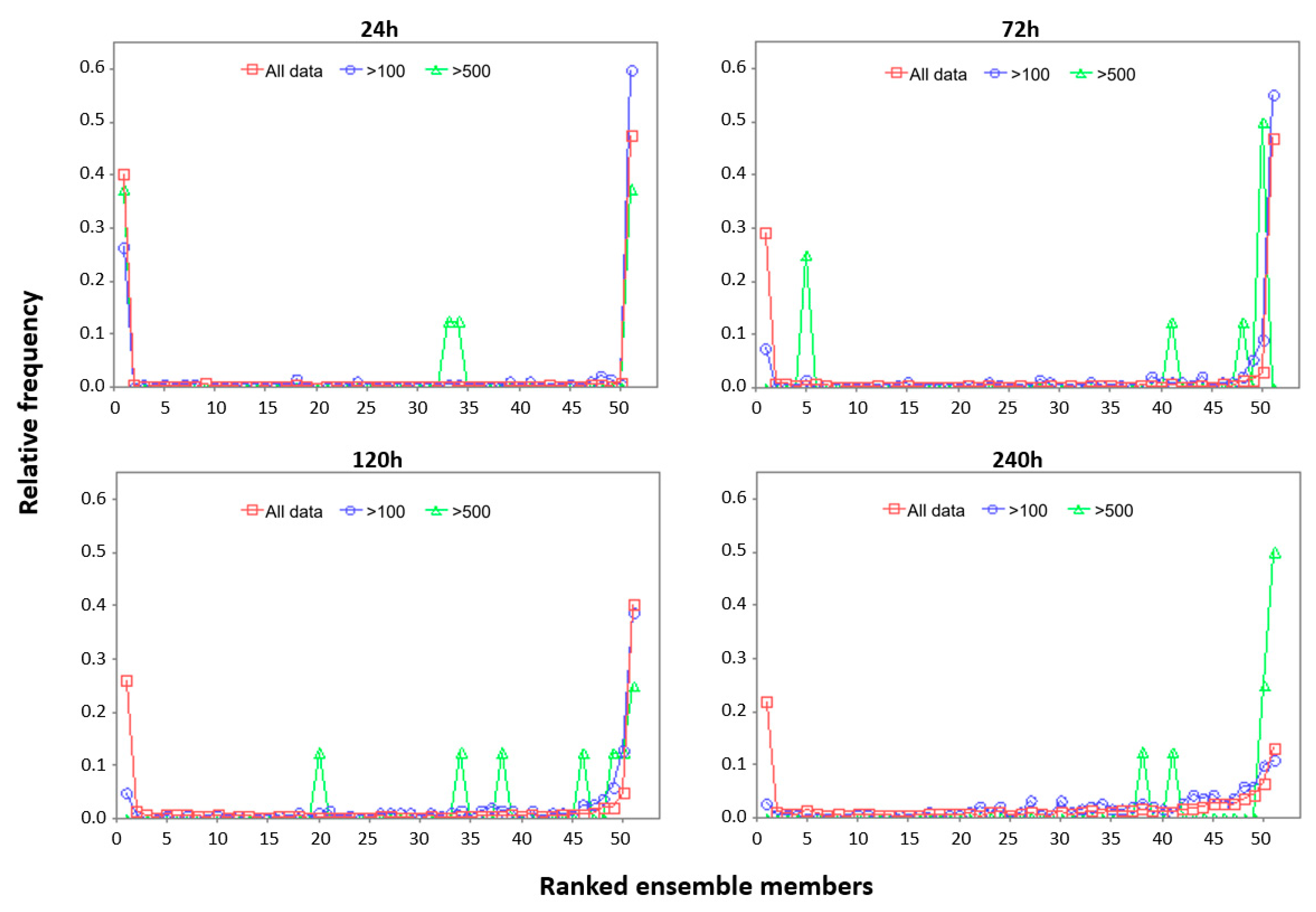
The results presented for the MAE, RME, MCRPS and RH evaluation methods were obtained from the total data (“all data”) for the analysis period and from the smallest data samples, which contain only the values of inflows occurring above the two thresholds defined in Section 2.2. Regarding to the BS index and the ROCD diagram, the presented results were obtained only for each of these two smallest sampling data cases. Since the RH and ROCD diagrams generate a graph for each forecast horizon, only four instances were chosen for the presentation of the respective results: 24 h, 72 h, 120 h and 240 h

3.3.1. Mean Absolute Error (MAE)

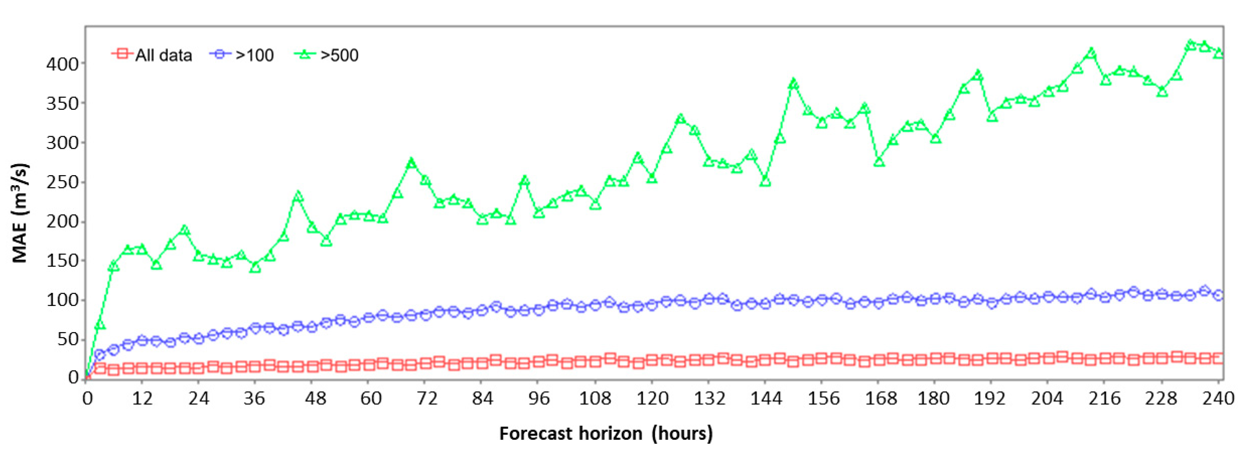
The results of the MAE statistical metric are shown in Figure 4. As can be inferred from Figure 4, and as would be expected, the MAE values increase with time over the forecast horizon, as well with the reduction of the data sampling size, taking into account the samples with data above the established thresholds. Considering the full dataset, the errors ranged from 15 m3/s to approximately 30 m3/s. On the other hand, considering the sampling data sets above the defined thresholds, the errors reached values close to the corresponding thresholds: 95 m3/s for the lowest threshold (100 m3/s) and close to 440 m³/s for the highest threshold (500 m3/s). The results for the initial period of forecast horizons are more strictly constrained by the initial conditions introduced in the prediction models, and therefore consistently report errors closer to zero.

3.3.2. Relative Mean Error (RME)

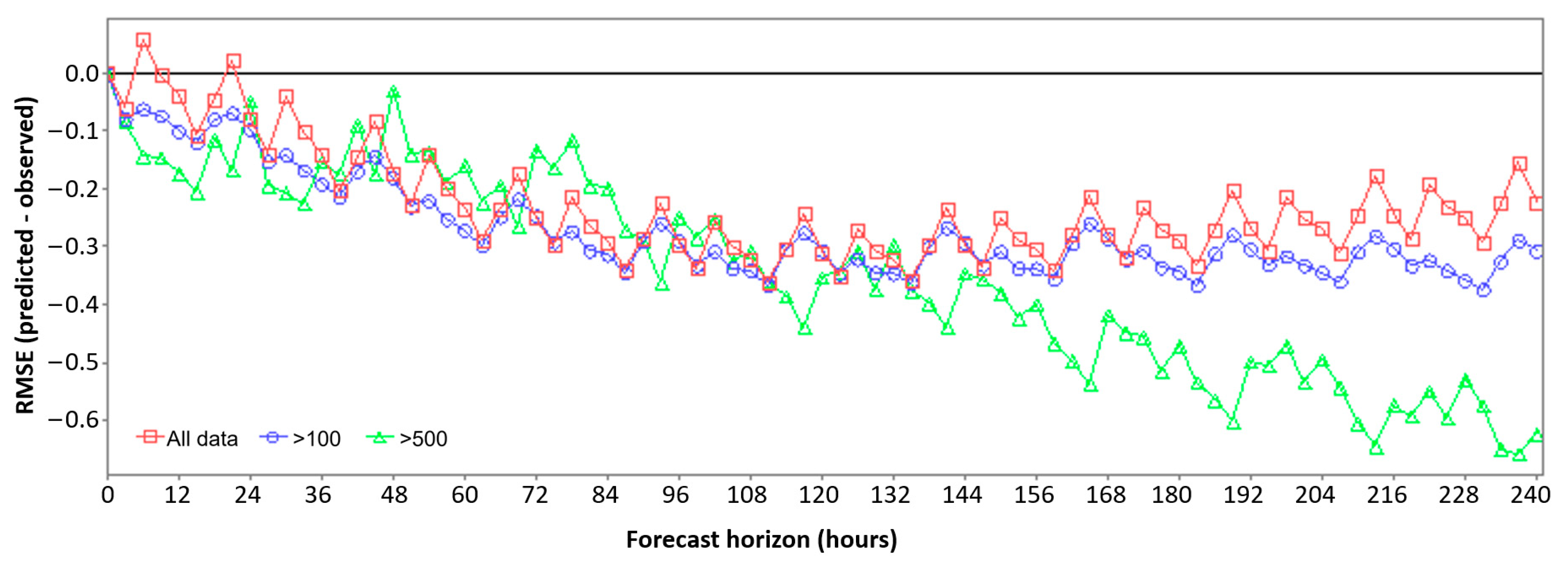
The results of the RME are shown in Figure 5. From the absolute values of the RME, it is noticeable that forecasts’ relative error increases with the forecast time horizon, especially up to approximately 120 h. From this prediction period onwards, the RME stabilizes for the complete data sampling set and for the sampling set with data above the lower threshold previously established. In effect, the RME values for the two sampling data sets prove quite similar throughout the forecast time period. For the sampling set with data above the highest threshold, the RME increases continuously over the entire forecast time period. Approximately, up to the 120th hour of the forecast horizon, the RME values for the three data sampling sets are similar.
Negative RME results indicate that, on average for the analyzed data, the mean values of the ensemble forecasts are lower than the respective observed values. According to Figure 5, the corresponding deviations ranged from zero to approximately 30% for the two largest sampling data sets, and reached values close to 60% for the smaller data set (highest threshold). Based on this evidence, we could conclude that the average of the ensemble forecasts underestimates the observed values. However, the existing deviation is, on average, limited to 30% up to 120 h (5 days) from the beginning of the forecast time period, for all the three data sampling sets considered (i.e., being almost irrelevant if the sampling data is limited by the thresholds for that initial 120 hours’ period). In view of all the uncertainties in the forecasting process, that deviation was considered acceptable.

3.3.3. Mean Continuous Rank Probability Score (MCRPS)

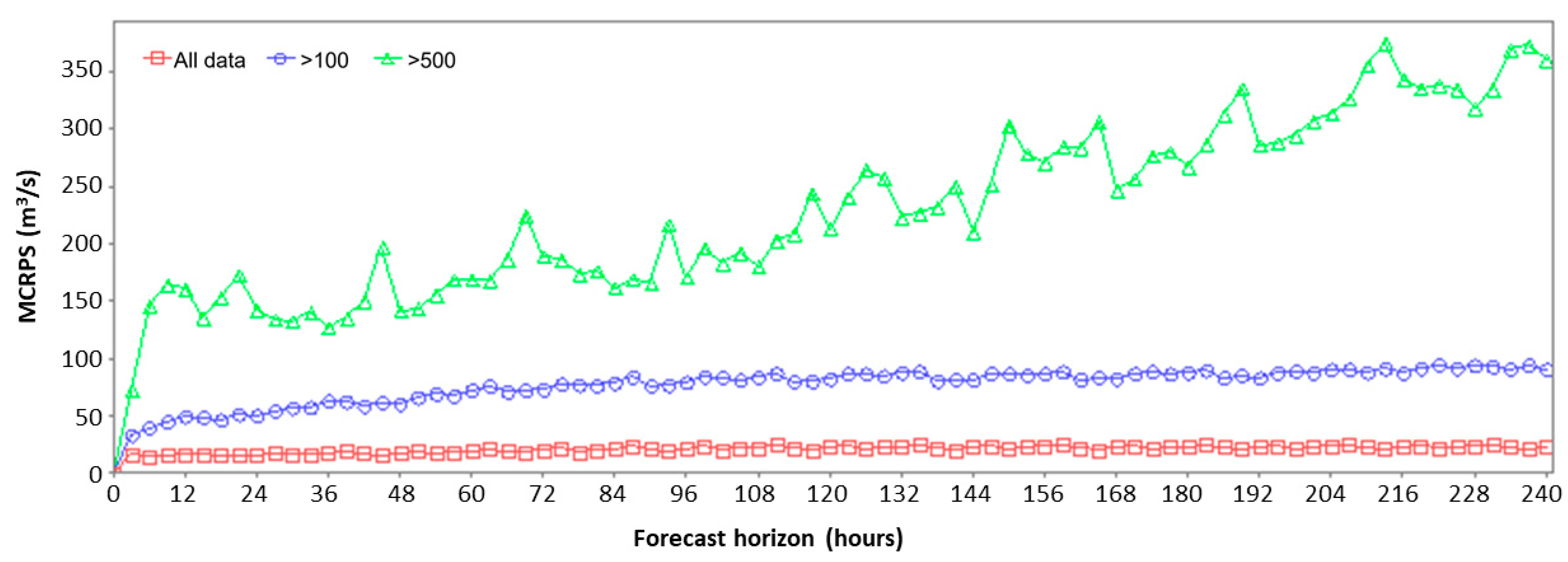
The results obtained for the MCRPS statistics—which translates the quality of a prediction per ensemble into a single error value—are presented in Figure 6. Unlike the previously shown metrics, which consider only the ensembles’ mean, the MCRPS considers all the values of the forecasts’ distribution. As the time development and values of the results due to the three sampling sets are similar to the corresponding ones obtained with the MAE (Figure 4), the analysis of the results would lead to conclusions similar to those stated before for the MAE. The errors obtained with the MCRPS are, however, slightly lower for all three sampling datasets. These results, combined with the conclusions obtained for the RME, enable the conclusion that the forecast values above the average of the ensemble are, in general, closer to the corresponding observed values.

3.3.4. Brier Score (BS)

Figure 7 shows the results obtained for the BS index, which allows the evaluation of the error with which discrete events (such as the exceedance of a threshold) are predicted through the distribution of ensemble forecasts. Taking these results into account and similar to the previous observations for the MAE and MCRPS statistics, the BS results also exhibit a general increase of the forecast errors with the increase of the forecast horizon. However, the analysis of this index indicates that there are more errors in the forecast of the exceedance for the lower threshold than for the upper threshold. Even so, the maximum value reached by this index was approximately 0.08, which is a value very close to the optimal result (BS = 0). These results lead to the conclusion that actual occurrences of inflows above the defined thresholds have a very high probability of being correctly predicted by means of the ensemble forecasts.

3.3.5. Rank Histogram (RH)

The Rank Histograms corresponding to different forecast horizons are presented in Figure 8. As can be seen in this figure, for the shortest forecast time displayed (corresponding to 24 h) the histogram generally displays an “U” format, which indicates that the corresponding observations frequently occurred above and below the ensemble forecasted range of values. However, in these cases a slight negative bias (rightward shift) is observed, which corresponds to the existence of more cases in which the observed values were above the ensemble’s maximum value, rather than below the minimum value. As the forecast time increases, there is a greater tendency for histograms to take an “inverted L” format, which indicates that the bias of the analyzed data is clearly negative, that is, the observations were more often above than below the 75th percentile of the ensemble forecasts. This inference reinforces the conclusions previously obtained for the error measures calculated with the mean values of the ensemble forecasts, namely the RME analysis.
For the larger forecast horizon (240 h), the histogram shows a greater spread of the observations, although a negative bias of the predictions is still noticeable. This is related to the existence of a greater dispersion of forecasts for the longer forecast periods because the wider the forecast range, the greater the probability of the observation being within that range.

3.3.6. Relative Operating Characteristic Diagram (ROCD)

Figure 9 shows the ROCD diagrams for each of the two threshold sampling data cases considered, for different times in the forecast horizon period. Like the BS index, this statistical evaluation of the quality of ensemble forecasts also focuses on the occurrence of discrete events, corresponding to the exceedance of the defined thresholds. As is shown in Figure 9, all the data points in the four graphs are located below 0.3 (on the abscissa axis), which means that the number of forecasted events above the pre-defined thresholds that were not effectively observed is small, i.e., that the probability of occurrence of false alarms in the analyzed forecasts is generally very low. However, according to Figure 9, probability of occurrence increases with the increase in the forecast time horizon and the order number of the ensemble members, which is also related to the ensemble’s forecasted range of values. Regarding the probability of detection of the magnitude of pre-established events, it does not change significantly with the time over forecast horizon, but it increases significantly with the rise in the order number of the ensemble members. According to the diagrams shown in Figure 9, the upper members of the ensemble forecasts present a probability of detection of the predefined events (occurrences above the established thresholds) above 70% and a probability of detecting false events below 30%.

4. Conclusions

Taking into account the inferences drawn from the analysis of the results of each of the statistical method applied and presented in the previous section and in the absence of reference criteria to systematically classify the quality of the ensemble forecasts based on those results, it may be concluded that the ensemble inflows forecasts used and evaluated in this work have demonstrated to be, in general, of good quality to detect the occurrence of flows above the pre-established thresholds, especially when those thresholds correspond to higher percentiles of the ensemble. Concerning the prediction of the magnitude of the events, it was concluded that, in general, the average of the ensemble forecasts underestimates the corresponding observed values, although the expected deviation is, on average, only approximately 30% for a forecast time up to 120 h. The values corresponding to the upper percentiles of the ensemble forecasts range also exhibit a negative deviation, especially in the initial forecast horizons, since there were many cases (more than 40% of cases, for prediction periods up to 120 h) in which the observed values were above the ensemble forecasted range of values, as shown in the Rank Histograms (Figure 8). However, considering only the upper percentiles of the forecasts above the average of the ensemble, the deviations will necessarily be less than 30%, which by itself can be considered acceptable in light of all the uncertainties inherent to the forecasting process. The forecast of the inflows to reservoirs can significantly contribute to the improvement of the reservoirs’ operational management. Therefore, the present work is of great importance to assess the degree of confidence that can be expected from the forecasts employed. The conclusions derived from the analysis above made it possible to define that the reference forecasts to be taken for the management of the Aguieira reservoir should be composed of:
(i)
A maximum ensemble value in the first 72 h, which corresponds to the most conservative solution with the lowest associated error, compared to the use of a lower percentile;
(ii)
The 75th percentile of the ensemble forecasts in the following hours (from 72 to 240 h), which is a more conservative operational guideline and exhibits a lower relative mean error compared to the use of the mean values of the ensemble forecasts, and, on the other hand, corresponds to a probability of detecting false alarms lower than the use of the maximum ensemble value. In fact, and since the predictions above 72 h show greater dispersion, the 75th percentile (whose values are between the mean value and the ensemble maximum value) was selected as a reference since it minimizes the triggering of unnecessary measures for the control of floods, caused by false alarms, and at the same time preserves a good performance in the detection of true alarms. In addition, the deviations in the reference forecast after the 72hour forecast will not have a significant impact on the operational management of the reservoir since the errors can be minimized with the next day’s forecast.

Author Contributions

Conceptualization, methodology development and application, J.M.; result analysis and validation, J.M. and R.M.; writing—original draft preparation, J.M.; writing—review and editing, R.M. and J.M.; supervision, R.M. All authors have read and agreed to the published version of the manuscript.

Funding

This research was funded by Portuguese Foundation for Science and Technology (PhD grant reference SFRH/BD/65905/2009, supported by “Programa Operacional Potencial Humano do Fundo Social Europeu” (POPH/FSE) funding).

Data Availability Statement

The data presented in this study are available on request from the corresponding author. The data is not publicly available due to the source data used being private and subject to restricted access.

Acknowledgments

The authors thank ECMWF and EDP-Produção for providing the base data used in this study and Pedro Pinto de Sousa for linguistic revision.

Conflicts of Interest

The authors declare no conflict of interest.

References

  1. Ramos, M.; Bartholmes, J.; Thielen, J. Development of decision support products based on ensemble forecasts in the European Flood Alert System. Atmos. Science Lett. 2007, 8, 113–119. [Google Scholar] [CrossRef]
  2. ECMWF. IFS Documentation CY33R1-Part V: Ensemble Prediction System. In IFS Documentation CY33R1; ECMWF: Reading, UK, 2009; Volume 5, pp. 1–25. [Google Scholar] [CrossRef]
  3. Cloke, H.; Pappenberger, F. Ensemble flood forecasting: A review. J. Hydrol. 2009, 375, 613–626. [Google Scholar] [CrossRef]
  4. Nobert, S.; Demeritt, D.; Cloke, H. Using Ensemble Predictions for Operational Flood Forecasting: Lessons from Sweden. J. Flood Risk Manag. 2010, 3, 72–79. [Google Scholar] [CrossRef]
  5. Bao, H.; Zhao, L.; He, Y.; Li, Z.; Wetterhall, F.; Cloke, H.; Pappenberger, F.; Manful, D. Coupling ensemble weather predictions based on TIGGE database with Grid-Xinanjiang model for flood forecast. Adv. Geosci. 2011, 29, 61–67. [Google Scholar] [CrossRef] [Green Version]
  6. Fan, F. Ensemble Forecast of Inflows to Reservoirs in Large Brazilian River Basins. Ph.D. Thesis, Federal University of Rio Grande do Sul-Institute of Hydraulic Research, Porto Alegre, Brazil, 2015. (In Portuguese). [Google Scholar]
  7. Mendes, J. Ph.D. Thesis, Faculty of Engineering of University of Porto, Porto, Portugal, 2017. (In Portuguese).
  8. Ramos, M.; Thielen, J.; Pappenberger, F. Utilisation de la prévision météorologique d’ensemble pour la prévision hydrologique opérationnelle et l’alerte aux crues. In Proceedings of the Colloque SHF-191º CST-“Prévisions hydrométéorologiques”, Lyon, France, 18–19 November 2008. [Google Scholar]
  9. Wu, W.; Emerton, R.; Duan, Q.; Wood, A.W.; Wetterhall, F.; Robertson, D.E. Ensemble flood forecasting: Current status and future opportunities. WIREs Water 2020, 7, e1432. [Google Scholar] [CrossRef]
  10. Alemu, E.; Palmer, R.; Polebitski, A.; Meaker, B. A Decision Support System for Optimizing Reservoir Operations Using Ensemble Streamflow Predictions. J. Water Res. Plann. Manag. 2011, 137, 72–82. [Google Scholar] [CrossRef]
  11. Fan, F.; Schwanenberg, D.; Collischonna, W.; Weerts, A. Verification of inflow into hydropower reservoirs using ensemble forecasts of the TIGGE database for large scale basins in Brazil. J. Hydrol. Region. Stud. 2015, 4, 196–227. [Google Scholar] [CrossRef] [Green Version]
  12. Arsenault, R.; Côte, P. Analysis of the effects of biases in ensemble streamflow prediction (ESP) forecasts on electricity production in hydropower reservoir management. Hydrol. Earth Syst. Sci. 2019, 23, 2735–2750. [Google Scholar] [CrossRef] [Green Version]
  13. Peng, A.; Zang, X.; Peng, Y.; Xu, W.; You, F. The application of ensemble precipitation forecasts to reservoir operation. Water Suppl. 2019, 19, 588–595. [Google Scholar] [CrossRef]
  14. Delaney, C.J.; Hartman, R.K.; Mendoza, J.; Dettinger, M.; DelleMonache, L.; Jasperse, J.; Ralph, F.M.; Talbot, C.; Brown, J.; Reynolds, D.; et al. Forecast informed reservoir operations using ensemble streamflow predictions for a multipurpose reservoir in Northern California. Water Res. Res. 2020, 56, e2019WR026604. [Google Scholar] [CrossRef]
  15. Cassagnole, M.; Ramos, M.H.; Zalachori, I.; Thirel, G.; Garçon, R.; Gailhard, J.; Ouillon, T. Impact of the quality of hydrological forecasts on the management and revenue of hydroelectric reservoirs–a conceptual approach. Hydrol. Earth Syst. Sci. 2021, 25, 1033–1052. [Google Scholar] [CrossRef]
  16. Coustau, M.; Rousset-Regimbeau, F.; Thirel, G.; Habets, F.; Janet, B.; Martin, E.; Saint-Aubin, C.; Soubeyroux, J. Impact of improved meteorological forcing, profile of soil hydraulic conductivity and data assimilation on an operational Hydrological Ensemble Forecast System over France. J. Hydrol. 2015, 525, 781–792. [Google Scholar] [CrossRef]
  17. Schaake, J.; Hamill, T.; Buizza, R.; Clark, M. HEPEX: The Hydrological Ensemble Prediction Experiment. Bullet. Am. Meteorol. Soc. 2007, 88, 1541–1547. [Google Scholar] [CrossRef]
  18. Murphy, A.H. What is a good forecast? An essay on nature of goodness in weather forecasting. Weather Forecast. 1993, 8, 281–293. [Google Scholar] [CrossRef]
  19. Hashino, T.; Bradley, A.A.; Schwartz, S.S. Evaluation of bias-correction methods for ensemble streamflow volume forecasts. Hydrol. Earth Syst. Sci. 2007, 11, 939–950. [Google Scholar] [CrossRef] [Green Version]
  20. Brown, J.; Demargne, J.; Seo, D.-J.; Liu, Y. The Ensemble Verification System (EVS): A software tool for verifying ensemble forecasts of hydrometeorological and hydrologic variables at discrete locations. Environ. Model. Softw. 2010, 25, 854–872. [Google Scholar] [CrossRef]
  21. Pappenberger, F.; Bogner, K.; Wetterhall, F.; He, Y.; Thielen, J. Forecast convergence score: A forecaster’s approach to analysing hydrometeorological forecast systems. Adv. Geosci. 2011, 29, 27–32. [Google Scholar] [CrossRef] [Green Version]
  22. Pappenberger, F.; Ramos, M.H.; Cloke, H.L.; Wetterhall, F.; Alfieri, L.; Bogner, K.; Salamon, P. How do I know if my forecasts are better? Using benchmarks in hydrological ensemble prediction. J. Hydrol. 2015, 522, 697–713. [Google Scholar] [CrossRef] [Green Version]
  23. Demargne, J.; Brown, J. HEPEX Science and Challenges: Verification of Ensemble Forecasts. HEPEX 2013. Available online: http://hepex.irstea.fr/hepex-science-and-challenges-verification-of-ensemble-forecasts/ (accessed on 3 August 2022).
  24. CAWCR. WWRP/WGNE Joint Working Group on Forecast Verification Research. Collaboration for Australian Weather and Climate Research; 2015. Available online: http://www.cawcr.gov.au/projects/verification/ (accessed on 3 August 2022).
  25. UNISDR. Guidelines for Reducing Flood Losses. A Contribution to the International Strategy for Disaster Reduction. United Nations Office for Disaster Risk Reduction, United Nations 2002. Available online: http://www.un.org/esa/sustdev/publications/flood_guidelines.pdf (accessed on 3 August 2022).
  26. Roebber, P.; Bosart, L. The complex relationship between forecast skill and forecast value: A real-world analysis. Weather Forecast. 1996, 11, 544–559. [Google Scholar] [CrossRef]
  27. Mendes, J.; Maia, R. Hydrologic modelling calibration for operational flood forecasting. Water Res. Manag. 2016, 30, 5671–5685. [Google Scholar] [CrossRef]
  28. Owens, R.G.; Hewson, T.D. ECMWF Forecast User Guide; ECMWF: Reading, UK, 2018. [Google Scholar] [CrossRef]
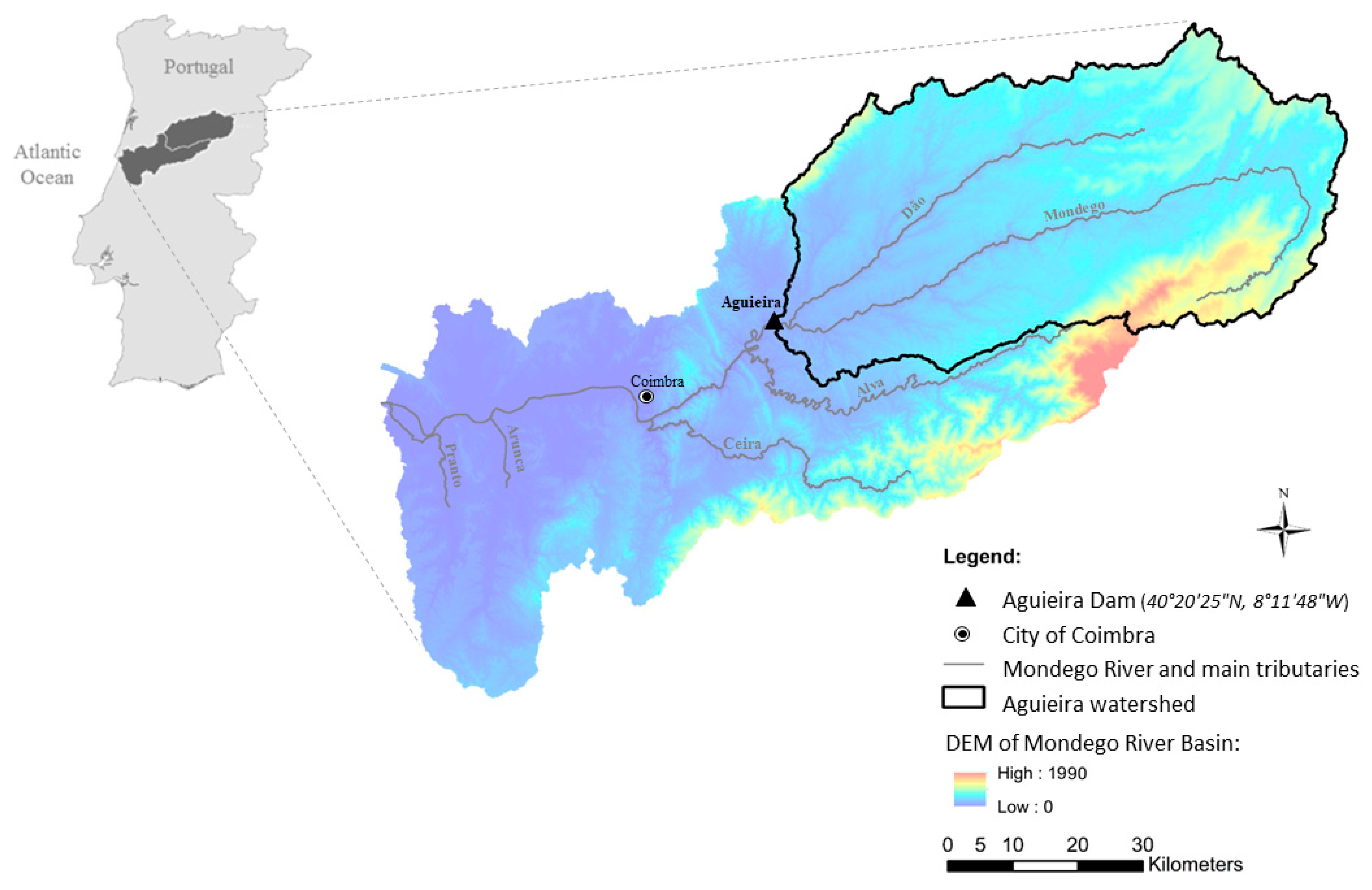
Figure 1. Location of the Aguieira reservoir and the corresponding watershed in the Mondego River Basin (in Portugal).
Hydrology 10 00028 g001
Figure 2. Comparison of the ensemble inflow forecasts to the Aguieira dam, in the 6 days before to the flood that occurred on 30 March 2013, with the corresponding observed inflows.
Hydrology 10 00028 g002
Figure 3. Maximum and mean values of the standard deviations obtained for each forecast horizon.
Hydrology 10 00028 g003
Figure 4. Results of the statistical metric MAE relative to the mean values of the ensemble inflow forecasts over the forecast time horizon, for different sets of data.
Hydrology 10 00028 g004
Figure 5. Results of the statistical metric RME relative to the mean values of the ensemble inflow forecasts over the forecast time horizon, for different sets of data.
Hydrology 10 00028 g005
Figure 6. Results of MCRPS of the ensemble inflow forecasts for each forecast horizon.
Hydrology 10 00028 g006
Figure 7. Results of BS of the ensemble inflow forecasts for each forecast horizon.
Hydrology 10 00028 g007
Figure 8. Rank Histograms of ensemble inflow forecasts for the forecast horizons of 24 h, 72 h, 120 h and 240 h.
Hydrology 10 00028 g008
Figure 9. ROCD of ensemble inflow forecasts for the forecast horizons of 24 h, 72 h, 120 h and 240 h.
Hydrology 10 00028 g009
Table 1. Statistical methods used to evaluate the quality of forecasts, per type of attribute considered, with: the respective classification in terms of the type of forecast to which it is applied—deterministic and/or by ensemble; focused (Y) or not (N) in exceeding a certain threshold and the description of the criteria which characterize an optimal quality (ideal result).
AttributeEvaluation MethodsType of ForecastOptimal Result
Total ErrorMAEDeterministic(N)Values equal to 0
MCRPSEnsemble(N)
BSEnsemble(Y)
BiasRMEDeterministic(N)
ReliabilityRHEnsemble(Y)Horizontally Uniform Histogram
DiscriminationROCDBoth(Y)Points located in the upper left corner of the diagram (POD = 1 and POFD = 0)
Disclaimer/Publisher’s Note: The statements, opinions and data contained in all publications are solely those of the individual author(s) and contributor(s) and not of MDPI and/or the editor(s). MDPI and/or the editor(s) disclaim responsibility for any injury to people or property resulting from any ideas, methods, instructions or products referred to in the content.