Abstract
Quebec has experienced a significant decrease in the amount of snow and an increase in temperature during the cold season. The objective of this study is to analyze the impacts of these climate changes on the spatio-temporal variability of the daily maximum flows generated by snowmelt in winter and spring using several statistical tests of correlation (spatial variability) and long-term trend (temporal variability). The study is based on the analysis of flows measured in 17 watersheds (1930–2019) grouped into three hydroclimatic regions. Regarding the spatial variability, the correlation analysis revealed that in winter, the flows are positively correlated with the agricultural area and the daily maximum winter temperature. In the spring, the flows are positively correlated with the drainage density and the snowfall but negatively correlated with the area of wetlands and the daily maximum spring temperature. As for temporal variability (long-term trend), the application of eight statistical tests revealed a generalized increase in flows in winter due to early snowmelt. In the spring, despite the decreased snow cover, no negative trend was observed due to the increase in the spring rainfall, which compensates for the decrease in the snowfall. This temporal evolution of flows in the spring does not correspond to the predictions of climate models. These predict a decrease in the magnitude of spring floods due to the decrease in the snowfall in southern Quebec.
1. Introduction
In regions with cold temperate climates (cold, snowy winters and hot, dry summers), the most significant freshets and associated floods were caused by snowmelt. Due to global warming, these regions still tend to see less snow in winter, the hydrological impacts of which lead to decreased freshet flows during spring snowmelt (e.g., [1,2,3,4,5,6]). Thus, among others, Blöschl et al. [3] clearly demonstrated that in Eastern Europe, a region characterized by this type of cold temperate climate, the decrease in the snowfall due to global warming has caused a significant decrease in the magnitude of spring flood flows generated mainly by the melting snow.
On the other hand, in these same climatic regions, in winter, warming associated with more frequent rainfall and early snowmelt should lead to increased winter daily maximum flows (e.g., [1]). Thus, the decrease in the magnitude of spring flood flows is partly offset by the increase in that of winter floods, which are becoming more and more frequent. However, very few studies have attempted to compare the temporal variability of the magnitude of flood flows generated by snowmelt in spring and winter in these cold temperate climatic regions to test this hypothesis along with the rising temperature.
In Quebec, a region also characterized by a cold temperate climate, several climate models have already predicted such an evolution in the magnitude of flood flows generated mainly by snowmelt in spring and winter in the current context of global warming [7]. However, there is still no one who has already been interested in verifying this hypothesis, despite the fact that several studies have already demonstrated the decrease in the amount of snowfall and the increase in temperature ([8,9,10]) during the cold season. Most of the work published on the temporal variability of floods in Quebec and Canada has focused exclusively on annual daily maximum flows generated mainly by spring snowmelt (e.g., [11,12,13,14,15,16,17]). Nevertheless, Beauchamp et al. (2015) analyzed the temporal variability of maximum daily flows in winter. The main objective of this study was to determine the climatic indices which influence the temporal variability of these flows. Thus, the effects of short (STP)- and long (SLP)-term persistence on the stationarity of the hydrological series analyzed were not taken into account. The conclusion of this study on the stationarity of the hydrological series analyzed, thus, deserves to be re-examined in the light of these two types of robust statistical tests.
In addition, the characteristics of floods are also significantly influenced by physiographic factors and land use, as several studies have already shown. These different factors can amplify or attenuate the effects of global warming on flood characteristics [6,18]. However, in Quebec, there is still no study on the impacts of these factors on the spatial variability of the magnitude of flood flows generated by snowmelt in winter and spring. This aspect is important because it will make it possible to determine the influence of these factors on the sensitivity of watersheds to changes induced by changes in precipitation and temperature regimes due to global warming.
In view of these considerations, the general objective of our study is to analyze the impacts of the decrease in snow cover on floods during the cold season (winter and spring) on the one hand, and the following specific objectives, on the other hand:
(i) Compare the temporal variability of seasonal daily maximum flows in winter and spring. This objective is based on the following hypothesis: the rise in temperature at the origin of the early snowmelt in winter and the significant decrease in the amount of snowfall in winter and spring have led to a significant increase in the magnitude of the flows daily maximums in winter to the detriment of that of the maximum daily flows in spring. There is therefore a negative correlation between the temporal variability of flows in winter and in spring;
(ii) Compare the factors that influence the spatial variability of the magnitude of daily maximum flows in winter and spring. The assumption underlying this objective is as follows: the magnitude of the maximum daily flows in winter and spring is influenced by the same physiographic and land-use factors because these flows are generated mainly by snowmelt, the effects of which can be amplified depending on the rainfall, during both seasons;
(iii) Determine whether these physiographic and land-use factors that influence the spatial variability of the magnitude of daily maximum flows during the two seasons amplify or attenuate the effects induced by global warming (temporal variability);
(iv) Finally, determine the impacts of short (STP)- and long (SLP)-term persistence on the stationarity of the series of the magnitude of the daily maximum flows during the two seasons.
2. Materials and Methods
2.1. Station Descriptions and Data Sources
We analyzed the flows in 17 watersheds across three hydroclimatic regions, which were established based on flow, temperature and precipitation patterns in southern Quebec [11] (Table 1 and Figure 1). The watersheds were chosen because the daily flow measurements of each spanned more than 85 years with no significant disturbances caused by human activity. The first southwest hydroclimatic region is located on the north shore and is characterized by a temperate continental climate. The watersheds in this region lie almost entirely in the Canadian Shield, which consists mainly of metamorphic and Precambrian mafic rocks. These rocks are often covered by surficial deposits of glaciofluvial origin (sand and gravel). The watersheds on the south shore of the St. Lawrence River were grouped into two hydroclimatic regions, one located north (maritime temperate climate) and one south (mixed temperate climate) of 47° N. They drain the Appalachians, an eroded mountain range consisting of sedimentary rocks, and the St. Lawrence Lowlands, a topographically flat geological formation consisting mainly of sedimentary rocks, also of marine, river and glacial origin.

Table 1.
Description of the stations studied.
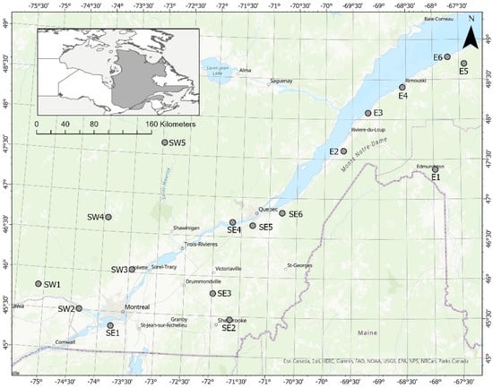
Figure 1.
Locations of the river stations. SE = Southeastern Hydroclimatic Region; E = Eastern Hydroclimatic Region; SW = Southwestern Hydroclimatic Region.
Daily flow data for these 17 rivers were taken from the website of the Ministère d’Environnement et de Lutte contre les changements climatiques du Québec’s Centre d’expertise hydrique du Québec (https://www.cehq.gouv.qc.ca/index_en.asp, accessed on 20 February 2020). The physiographic data of the watersheds come from the database of the Glaciolab laboratory at the University of Quebec at Trois-Rivières.
They have already been described in detail by [19] in particular. These data were supplemented by those extracted from the database published by [20] with particular regard to data on the areas of wetlands. It is important to note that the areas of wetlands include those of different types of wetlands (ponds, swamps, bogs, peatlands, floodplains, etc.) and small lakes, as well as those of other bodies of water and depressions that can contribute water surface runoff. It is important to remember that the objective of our study is not to determine the influence of each type of wetland or other body of water, but to determine the influence of the surface area they occupy in a watershed on the magnitude of the flows. Climate variables were obtained from the Environment Canada website (https://climat.meteo.gc.ca/climate_normals/index_f.html, accessed on 18 June 2021). These are the averages of the monthly climatic averages calculated over the following two periods: 1971–2000 and 1981–2010. The physiographic and climatic data analyzed are shown in Table 2.
Table 2.
Correlation coefficients calculated between physiographic variables and magnitude (L/s/km²) of winter and spring maximum daily flows from 1930–2019.
2.2. Data Analysis
2.2.1. Analysis of Spatial Variability of Seasonal Daily Maximum Flows
For each river, we compiled a series of winter (January to March) and spring (April to June) daily maximum flows, the highest values measured in both seasons from 1930–2019. We calculated the arithmetic mean (Qmean) for each series and compared the means of the 17 rivers using parametric (ANOVA) and non-parametric (Kruskal–Wallis) tests. Given the varying surface areas of the watersheds, we converted daily flows into specific flows (L/s/km²), then correlated the means with the seasonal and physiographic climate variables of the watersheds (see Table 2).
2.2.2. Analysis of Temporal Variability (Long-Term Trend) of Seasonal Daily Maximum Flows
We used nine different statistical tests to compare the long-term trend of daily maximum flow in winter and spring. These tests are described in detail in the scientific literature (e.g., [21,22,23,24,25]). This temporal variability analysis was carried out in the following steps:
- -
- The original Mann–Kendall (MK) test was applied in the first step. Its mathematical description and application in hydroclimatology were outlined in detail by [26]. The purpose of this test was to detect the long-term trend of a non-autocorrelated hydroclimatic series;
- -
- Given that the original MK test did not account for short-term and long-term persistence effects (STP and LTP), two tests were applied in the second step to eliminate the following short-term persistence effects: the prewhitening method (MMK-PW) tests, developed by [27], and the trend-free prewhitening method (TFPW) tests described by [28]. The purpose of both tests was to eliminate autocorrelation in the series data;
- -
- Two tests were applied in the third step to correct the effects of autocorrelation on the variance; both tests were modified Mann–Kendall tests (MMK) developed by [29,30];
- -
- The long-term persistence (LTP) test was applied in the fourth step to eliminate the effects of long-term persistence. Developed by [31,32], the test’s application has been described in detail, notably by [22];
- -
- To detect breaks in the means, two statistical tests were applied at the fifth stage: Pettitt’s tests as described in [33,34]. The first test exclusively detects abrupt breaks while the second test considers abrupt and progressive breaks;
- -
- Finally, the regional MK test was applied in the last step to eliminate the spatial autocorrelation (cross-correlation) effects described by [35,36]. However, the results of the latter are not presented here because no significant spatial autocorrelation was observed.
3. Results
3.1. Comparison of Spatial Variability of Winter and Spring Daily Maximum Flows and Correlation Analysis
Daily means maximum flow (expressed as specific flows) in winter and spring are shown in Figure 2. In winter, the highest flow values were observed in the southeast hydroclimatic region (SE1 to SE6) south of 47° N on the south shore. The mean values of these flows were greater than 80 L/s/km² in this region, but less than 50 L/s/km² in the other two hydroclimatic regions (E1 to E6 and Sw1 to SW5). In spring, the mean flow values of rivers in the southwest hydroclimatic region (SW1 to SW5) on the north shore of the St. Lawrence River were lower than those on the south shore. These means were all below 179 L/s/km², but most rivers on the south shore far exceeded this threshold (Figure 2).
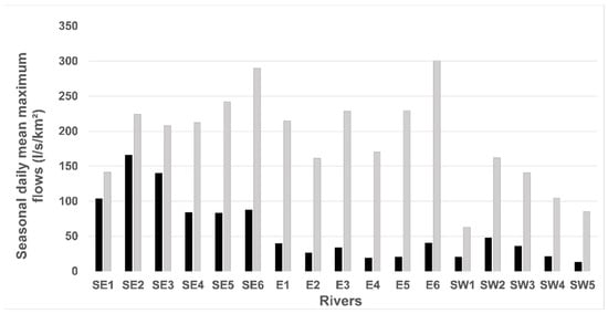
Figure 2.
Comparison of maximum daily flow means in winter (black bars) and spring (grey bars).
The results of the analysis of the correlation between maximum daily flow means and physiographic factors (Table 2) showed that in winter, average flow values were only significantly correlated with agricultural areas in the watersheds. This correlation was positive. In spring, they were negatively correlated with wetlands (the highest correlation value) but positively correlated with drainage density and agricultural area. As for climatic variables, in winter, the daily maximum flows are positively correlated with the winter daily maximum temperature. In spring, they are positively correlated with the amount of snowfall but negatively correalted with the daily maximum temperature during the cold season.
3.2. Comparison of Temporal Variability (Stationarity) of Winter and Spring Maximum Daily Flows
The results of applying six tests regarding long-term trend analysis are shown in Table 3 and Table 4 for winter and spring, respectively. In winter, these results are consistent. Indeed, these tests clearly show that the hydrological series of 15 of the 17 rivers analyzed were affected by a significant long-term trend (Table 3 and Figure 3, Figure 4 and Figure 5). The change was widespread on both shores of the St. Lawrence River. These changes result in a significant increase in maximum daily flows over time (positive trend). An example of this increase is given in Figure 3.
Table 3.
Results of the various Mann–Kendall tests applied to daily maximum flow series in winter from 1930–2019.
Table 4.
Results of the various Mann–Kendall tests applied to daily maximum flow series in spring from 1930–2019.
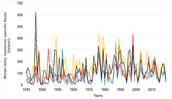
Figure 3.
Interannual variability of winter daily maximum specific flows (L/s/km²) in the Southeastern hydroclimatic region from 1930 to 2019. Châteaugay River: red curve; Eaton River: yellow curve; Nicolet River: black curve; Etchemin River: blue curve; Beaurivage River: orange curve; Du Sud River: grey curve.
Figure 4.
Interannual variability of winter daily maximum specific flows (L/s/km²) in the Eastern hydroclimatic region from 1930 to 2019. Ouelle River: yellow curve; Du Loup River: orange curve; Trois-Pistoles River: red curve; Rimouski River: blue curve; Matane River: grey curve; Blanche River: black curve.
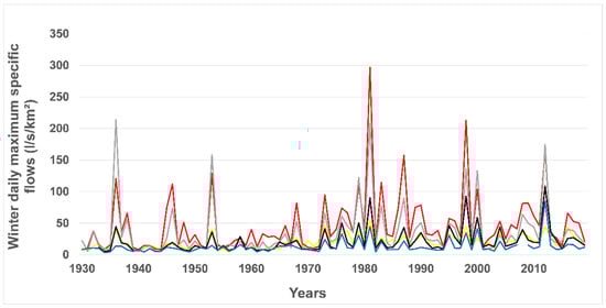
Figure 5.
Interannual variability of winter daily maximum specific flows (L/s/km²) in the Southwestern hydroclimatic region from 1930 to 2019. Petite Nation River: yellow curve; Du Nord River: Red curve; L’Assomption River: grey curve; Matawin River: black curve; Vermillon River: blue curve.
In spring, the test results are no longer consistent. The original MK test and those that eliminate the effects of short-term persistence revealed a significant positive long-term trend for the five rivers on the north shore (Figure 6) and seven of the rivers on the south shore, five of which were located north of 47° N and two south of 47° N (Table 4). It is very important to mention that, unlike the north shore, almost all statistically significant trends on the south shore were detected primarily by a single test (MMKY). However, the test that eliminates the effects of long-term persistence (LTP) revealed a significant long-term trend in three rivers only: two on the north shore and one on the south shore (north of 47° N). Taking into account the effects of the long-term trend (Hurst effect) on the stationarity of the hydrological series, the change in flows observed, therefore, became less widespread on the north shore in spring, in contrast with the results of the other tests. The Z values of all the tests are positive, with the exception of those of the Eaton and Rimouski rivers on the south shore. These values show an almost generalized upward trend in the magnitude of the maximum daily flows in spring and winter. This is an important result of this study.
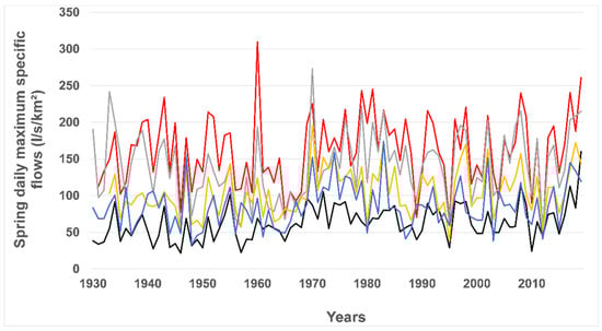
Figure 6.
Interannual variability of spring daily maximum specific flows (L/s/km²) in the Southwestern hydroclimatic region from 1930 to 2019. Petite Nation River: black curve; Du Nord River: Red curve; L’Assomption River: grey curve; Matawin River: orange curve; Vermillon River: blue curve.
The application of two tests (Pettitt and Lombard) to detect the breaks in the averages highlighted by the previous tests reveals that these breaks are almost abrupt, and all occurred before 1973 (Table 5). To verify whether winter and spring daily maximum flow series were affected by a second break in means, the six statistical tests were applied to analyze the series from 1975–2019. No changes were detected in the long-term trend or in the break in means (these results are not presented here). Therefore, the wet period of the 2010s, which was characterized by high-intensity freshets, did not significantly affect the means of the hydrological series.
Table 5.
Pettitt and Lombard test results applied to maximum daily flow series in winter and spring from 1930–2019.
Finally, the correlation between the maximum daily flows in winter and in spring was calculated. The results of this analysis are presented in Table 6. They revealed that for the three periods, we can conclude that in the majority of watersheds, there is no significant correlation between the magnitude of the maximum daily flows in winter and spring despite the general increase in this magnitude observed in winter. Nevertheless, some regional trends are worth highlighting. On the south shore (SE1 to SE6), south of 47° N, all the signs of correlation coefficients are negative. On the other hand, north of this parallel (E1 to E6), these signs become globally positive. On the north shore (SW1 to SW5), no correlation coefficient is statistically significant for the three periods.
Table 6.
Correlation coefficients calculated between the winter and spring daily maximum flows for three periods.
4. Discussion
4.1. Spatial Variability of Winter and Spring Maximum Daily Flows
Analysis of the spatial variability of maximum daily flows in winter and spring from 1930–2019 revealed a regional disparity across Quebec. In winter, rivers south of 47° N (SE1 to SE6) on the south shore had higher maximum daily flows than the rivers in other hydroclimatic regions. Maximum daily flow means were all greater than 80 L/s/km² in this region in winter, but less than 50 L/s/km² elsewhere. In spring, spatial disparity resulted in lower maximum daily flows on the north shore (SW1 to SW5) of the St. Lawrence River than on the south shore, where overall flow means were greater than 170 L/s/km², but were less than 170 L/s/km² on the north shore.
The correlation analysis between the flows revealed that many physiographic and climatic factors can explain this spatial disparity in flows. In winter, agricultural area in the watersheds and winter daily maximum temperature are the two factors positively correlated with winter daily maximum flows. Watersheds south of 47° N tended to have larger agricultural areas (>20%) than those in other hydroclimatic regions in Quebec. The impacts of agriculture on floods have already been extensively studied, even in Quebec (e.g., [37,38,39,40]). However, all of these studies focused on the impacts of agriculture on flood flows due to rainfall and sometimes snowmelt in spring. These conditions differ from those that cause winter floods due to total freezing of the ground and all water bodies. As such, the effect of evapotranspiration would not come into play in this context. Regardless, it is well-known that agriculture causes soil sealing, which promotes runoff from snowmelt in winter. However, soil sealing has also been observed in other regions due to extremely cold winters in Quebec. However, unlike non-agricultural watersheds, in agricultural watersheds, fields are plowed in late fall for seeding in spring after the snow melts. Thus, the soil of the fields remains completely bare (devoid of any plant cover). When snowmelt runoff occurs in winter, water runs off these bare soils more easily than any other type of terrain. This explains the higher flood flows in the more agricultural watersheds on the southern shore, in particular, those located south of 47° N. This melting of snow in winter results from the rise in temperature which also generates precipitation in liquid form (rain). This explains the positive correlation observed between winter daily maximum flows and winter daily maximum temperatures.
In spring, four factors influenced maximum daily flows: wetland area, drainage density, snowfall and spring daily maximum temperature. The correlation was negative with the wetlands area and daily maximum temperature but positive with the other two factors. The north shore watersheds with the largest wetland area (>8%) had the lowest maximum daily flows. The effects of this factor on the magnitude of freshets have already been analyzed in the scientific literature (see syntheses provided by [41,42,43]. These studies show that these effects varied from one watershed to the next because they depend on many intrinsic and extrinsic factors: area, topography, antecedent humidity conditions, water level, soil characteristics, type of plants and vegetation that colonize them, location in the watershed, seasonality, degree of connectivity with river channels, etc. Depending on these different factors, wetlands can cause the magnitude of floods to rise or fall. In Quebec, Blanchette et al. [44] demonstrated that the decrease in the area of wetlands in the St. Charles River watershed had caused a significant decrease in the magnitude of flood flows. This significant decrease in the magnitude of flood flows resulted from the well-known process of the “sponge effect” exerted by wetlands on water runoff and infiltration. However, in the context of this study, wetlands include other types of water bodies such as small lakes or other surface depressions present in the watersheds of Quebec due to the succession of glacial and interglacial periods that have sculpted its landscape. Under these conditions, we can no longer invoke this “sponge effect” to explain the negative correlation observed between the magnitude of spring daily maximum flows and the area of these wetlands. Rather, it is another effect called the “surface water storage effect”. The different landscape units (wetlands, lakes and other surface depressions) store surface water first from melting snow and then gradually release it to feed river channels. Thus, the magnitude of the flows remains low, but their duration is long, unlike the sponge effect exerted exclusively by typical wetlands. The surface water storage effect has already been described by several authors [45,46,47,48,49,50,51,52,53]. It has just been described in Quebec by [54,55] in four watersheds on both shores.
In Quebec, our results clearly showed that the larger the wetland area, the smaller the magnitude of spring freshets in the watershed. In contrast, watersheds with larger agricultural areas had fewer wetlands, as drainage increased significantly following the modernization of agricultural practices in Quebec since 1950 [56]. However, their drainage density networks increased overall, which promoted a relatively rapid concentration of runoff from snowmelt to the channels. This rapid transfer of runoff increased spring flood peaks, which were, thus, positively correlated with drainage density and agricultural area (the correlation between flow rates and agricultural area is significant at the 10% level). It should be noted that wetlands covered less than 4% of watersheds on the south shore, but more than 8% on the north shore.
Regarding climatic variables, spring floods were mainly brought on by snowmelt. The magnitude of their peak, therefore, depended on the accumulation of snow throughout the cold season, which explained the positive correlation between maximum daily flows and the amount of snowfall in winter and spring. As for the spring daily maximum temperature, this climatic variable favors the ablation of snow and the evaporation of water from the melt, thus contributing to the reduction in spring flood peaks (negative correlation). In addition, relatively warm springs are generally dry and often follow winters with early snowmelt in Quebec [17].
4.2. Temporal Variability of Winter and Spring Maximum Daily Flows
Analysis of long-term trends in the maximum daily flows of the series showed a clear difference between winter and spring in southern Quebec. In fact, eight different statistical tests showed that in winter, almost all of the rivers (88%) had a significant increase in maximum daily flows, whereas in spring, only 18% of the rivers analyzed had an increase. As such, it seems clear that a significant widespread change in maximum daily flows occurred in winter across southern Quebec. Two hypotheses could be used to explain this increase in maximum daily flow means in winter.
- -
- The increase in temperatures during the winter in southern Quebec. This increase has already been observed by several authors [9,10]. This increase would, thus, cause an early melting of snow which would be at the origin of the increase in the maximum daily flows in winter. Early snowmelt has been observed in many parts of North America (e.g., [13,15,57,58,59,60]);
- -
- The increased frequency of precipitation in the form of rain. Such an increase would likely have caused the increase in the magnitude of winter maximum daily flows. This increase was observed in a few watersheds analyzed as part of this study, both on the south shore and on the north shore (the results are not presented here).
In the spring, the significant decrease in the snowfall during the cold season did not lead to a decrease in spring daily maximum flows. In fact, long-term trend analysis has clearly shown that a hydrological series of flows is not affected by a negative trend in the three hydroclimatic regions. Thus, most of the hydrological series have remained stationary; others have been affected by a positive trend (increase in flows). This absence of any negative trend despite the decrease in the amount of snow can be explained by the increase in the spring rainfall. This rainfall increased in spring in the three hydroclimatic regions [10]. This increase, thus, compensates for the decrease in the amount of snow. In addition, rain accelerates snowmelt by increasing the peaks (spring daily maximum flows) of floods. This increase in the amount of rainfall was observed in some watersheds analyzed as part of this study, both on the south shore and on the north shore (the results are not presented here).
Finally, the results reveal that the upward trend in the magnitude of the spring daily maximum flows seems more generalized on the north shore than on the south shore. This can be explained by the fact that the very significant reduction in agricultural area that has occurred since 1950 in the agricultural watersheds of the south shore favors infiltration to the detriment of runoff. This argument is based on the fact that the spring daily minimum flows increase significantly over time in the most agricultural watersheds located south of 47° N (SE1 to SE6) on the south shore, while this increase is totally absent on the north shore (SW1 to SW5) [59,60]. It follows that changes in land use in the agricultural watersheds of the southern shore tend to attenuate the effects of warming on the increase in the magnitude of spring flood flows. On the other hand, in winter, the presence of bare soil in cultivated fields tends to promote runoff, thereby increasing the magnitude of winter flood flows that will become more and more frequent in southern Quebec.
5. Conclusions
Winter and spring daily maximum flows are mainly caused by snowmelt in southern Quebec. Analysis of the spatial variability of their magnitude revealed that the same physiographic and climatic factors were not at play in both seasons, even though the freshets were caused by snowmelt. In winter, the magnitude of these flows was influenced by agricultural area (positive correlation) and winter daily maximum temperature in the watersheds. As such, the highest flow magnitude values were observed in the agricultural watersheds of the hydroclimatic region south of 47° N (SE1 to SE6) on the south shore of the St. Lawrence River. This influence can be explained by agricultural practices which consist of leaving the soil bare in the fields in winter, thus promoting runoff during snowmelt. In the context of the rise in temperature and the amount of rain due to warming, these agricultural practices will amplify the intensity of winter floods, which will become more and more frequent in southern Quebec. In spring, the magnitude of maximum daily flows was mainly influenced by wetland areas (negative correlation) and snowfall (positive correlation). Wetlands store runoff water on the surface and gradually release it (surface water storage effect) to river channels. This process is slightly different from the classic sponge effect. The lowest magnitude values for these spring daily maximum flows were observed in watersheds on the north shore (SW1 to SW5) of the St. Lawrence River, where wetland areas were larger (>8%) than those on the south shore (<4%).
Analysis of the temporal variability in the magnitude of daily maximum flows using eight different statistical tests revealed an overall increase in winter across Quebec. This increase in magnitude was likely due to rising winter temperatures and rainfall. In the spring, the most significant result is the demonstration of the absence of any negative long-term trend in the hydrological series despite a significant decrease in the amount of snow. This decrease in snowfall is compensated by the increase in the rainfall due to the increase in temperature. The effects of this temperature increase on the temporal variability of flows seem more marked on the north shore than on the south shore. On the south shore, the significant reduction in agricultural area since the modernization of agriculture in 1950 has, over time, favored infiltration to the detriment of runoff, thus mitigating the increase in the intensity of spring floods.
In light of these results, the temporal evolution of the daily maximum flows in spring does not correspond to that predicted by climate models. These predict their decline in future decades due to the decrease in the amount of snow. However, these models do not integrate the increase in spring rainfall in their predictions.
As a general summary, the analysis of the seasonal daily maximum flows in the cold season (winter and spring) made it possible to draw up a global and precise portrait of their spatio-temporal variability in southern Quebec. With regard to spatial variability, the main factor in the variability of these flows is the wetlands area, with the exception of the winter season. During winter, the variability of flows is mainly influenced by the agricultural area. As for the temporal variability, it is characterized by a generalized tendency to increase flows during the four seasons, mainly due to the increase in rainfall in the context of generalized warming of the climate. However, this upward trend is more marked on the north shore than on the south shore. Thus, wetlands spatially attenuate the intensity of floods but increase their magnitude over time because their surface runoff water storage capacity does not increase over time as the amount of rainfall increases. Thus, unlike the minimum daily flows, the generalized decrease in snow cover due to the increase in temperature does not seem to affect the seasonal daily maximum flows due to the increased rainfall in southern Quebec.
Finally, the changes observed in the spatio-temporal variability of flows in the different watersheds will be associated later with the resulting ecological impacts in order to be able to establish ecological limits of hydrologic alteration (ELOHA) thresholds in order to be able to monitor their integrity in this context of climate change.
Author Contributions
Conceptualization: A.A.A.; methodology: A.A.A.; formal analysis: investigation: A.A.A.; writing—original draft preparation: A.A.A.; writing—review and editing, A.A.A.; funding acquisition, A.A.A. All authors have read and agreed to the published version of the manuscript.
Funding
This research was funded by the Natural Sciences and Engineering Research Council of Canada (NSERC), grant number 261274/2019.
Informed Consent Statement
Not applicable.
Data Availability Statement
The data presented in this study are available on request from the author.
Conflicts of Interest
The author declares no conflict of interest.
References
- Aygün, O.; Kinnard, C.; Campeau, S. Impacts of climate change on the hydrology of northern midlatitude cold regions. Prog. Phys. Geogr. Earth Environ. 2020, 44, 338–375. [Google Scholar] [CrossRef]
- Berghuisjs, W.R.; Aalbers, E.E.; Larsen, J.R.; Transcoso, R.; Woods, R.A. Recent changes in extreme floods across multiple continents. Environ. Res. Lett. 2017, 12, 114035. [Google Scholar] [CrossRef]
- Blöschl, G.; Hall, J.; Viglioni, A.; Perdigão, R.A.; Merz, B.; Lun, D.; Arheimer, B.; Aronica, G.T.; Bilibashi, A.; Boháč, M.; et al. Changing climate both increases and decreases European river floods. Nature 2019, 573, 108–111. [Google Scholar] [CrossRef] [PubMed]
- Buttle, J.M.; Allen, D.M.; Caissie, D.; Davison, B.; Hayashi, M.; Peters, D.L.; Whitfield, P.H. Flood processes in Canada: Regional and special aspects. Can. Water Resour. J. 2016, 41, 7–30. [Google Scholar] [CrossRef]
- Mallakpour, I.; Villarini, G. The changing nature of flooding across the Central United States. Nat. Clim. Chang. 2015, 5, 250–254. [Google Scholar] [CrossRef]
- Mangini, W.; Viglione, A.; Hall, J.; Hundecha, Y.; Ceola, S.; Montanari, A.; Rogger, M.; Salinas, J.L.; Borzi, I.; Parajka, J. Detection of trends in magnitude and frequency of flood peaks across Europe. Hydrol. Sci. J. 2018, 63, 493–512. [Google Scholar] [CrossRef]
- Boyer, C.; Chaumont, D.; Chartier, I.; Roy, A.G. Impact of climate change on the hydrology of St. Lawrence tributaries. J. Hydrol. 2010, 384, 65–83. [Google Scholar] [CrossRef]
- Brown, R.D. Analysis of snow cover variability and change in Québec, 1948–2005. Hydrol. Process. 2010, 24, 1929–1954. [Google Scholar] [CrossRef]
- Guerfi, N.; Assani, A.A.; Mesfioui, M.; Kinnard, C. Comparison of the temporal variability of winter daily extreme temperatures and precipitations in southern Quebec (Canada) using the Lombard and copula methods. Int. J. Climatol. 2015, 35, 4237–4246. [Google Scholar] [CrossRef]
- Yagouti, A.; Boulet, G.; Vincent, L.; Vescovi, L.; Mekis, E. Observed changes in daily temperature and precipitation indices for Southern Québec, 1960–2005. Atmos.-Ocean 2008, 46, 243–256. [Google Scholar] [CrossRef]
- Assani, A.A.; Charron, S.; Matteau, M.; Mesfioui, M.; Quessy, J.-F. Temporal variability modes of floods for catchments in the St. Lawrence watershed (Quebec, Canada). J. Hydrol. 2010, 385, 292–299. [Google Scholar] [CrossRef]
- Burn, D.H.; Whitfield, P.H. Changes in floods regimes in Canada. Can. Water Resour. J. 2016, 41, 139–150. [Google Scholar] [CrossRef]
- Cunderlik, J.M.; Ouarda, T.B.M.J. Trend in the timing and magnitude of floods in Canada. J. Hydrol. 2009, 375, 471–480. [Google Scholar] [CrossRef]
- Hodgkins, G.A.; Whitfield, P.H.; Burn, D.H.; Hannaford, J.; Renard, B.; Stahl, K.; Fleig, A.K.; Madsen, H.; Mediero, L.; Korhoneb, J.; et al. Climate-driven variability in the occurrence of major flood across North America and Europe. J. Hydrol. 2017, 552, 704–717. [Google Scholar] [CrossRef]
- Mazouz, R.; Assani, A.A.; Quessy, J.-F.; Légaré, G. Comparison of the interannual variability of spring heavy floods characteristics of tributaries of the St. Lawrence River in Quebec (Canada). Adv. Water Resour. 2012, 35, 110–120. [Google Scholar] [CrossRef]
- Zadeh, S.M.; Burn, D.H.; O’Brien, N. Detection of trends in flood magnitude and frequency in Canada. J. Hydrol. Reg. Stud. 2020, 28, 100673. [Google Scholar] [CrossRef]
- Beauchamp, M.; Assani, A.A.; Landry, R.; Massicotte, P. Temporal variability of the magnitude and timing of winter maximum daily flows in southern Quebec (Canada). J. Hydrol. 2015, 529, 410–417. [Google Scholar] [CrossRef]
- Tramblay, Y.; Mimeau, L.; Neppel, L.; Vinet, F.; Sauquet, E. Detection and attribution of flood trends in Mediterranean basins. Hydrol. Earth Syst. Sci. 2019, 23, 4419–4431. [Google Scholar] [CrossRef]
- Kinnard, C.; Bzeouich, G.; Assani, A. Impacts of summer and winter conditions on summer river low flows in low elevation, snow-affected catchments. J. Hydrol. 2022, 605, 127393. [Google Scholar] [CrossRef]
- Belzile, L.; Bérubé, P.; Hoang, V.D.; Leclerc, M. Méthode Écohydrologique de Détermination des Débits Réservés Pour la Protection des Habitats du Poisson Dans les Rivières du Québec; Rapport présenté par l’INRS-Eau et le Groupe-conseil Génivar inc; au Ministère de l’Environnement et de la Faune et à Pêches et Océans Canada: Quebec City, QC, Canada, 1997; 83p. [Google Scholar]
- Dinpashoh, Y.; Mirabbasi, R.; Jhajharia, D.; Abianeh, H.Z.; Mostafaeipour, A. Effect of short-term and long-term persistence on identification of temporal trends. J. Hydrol. Eng. ASCE 2014, 19, 617–625. [Google Scholar] [CrossRef]
- Kumar, S.; Duffy, C.J. Detecting hydroclimatic change spatio-temporal analysis of time series in Colorado River basin. J. Hydrol. 2009, 374, 1–15. [Google Scholar] [CrossRef]
- Kumar, S.; Merwade, V.; Kam, J.; Thurner, M. Streamflow trends in Indiana: Effects of long term persistence, precipitation and subsurface drains. J. Hydrol. 2009, 374, 171–183. [Google Scholar] [CrossRef]
- Quessy, J.F.; Favre, A.C.; Saïd, M.; Champagne, M. Statistical inference in Lombard’s smooths-change model. Environmetrics 2011, 22, 882–893. [Google Scholar] [CrossRef]
- Serinaldi, F.; Kilsby, C. The importance of prewhiting in change point analysis under persitence. Stoch. Environ. Res. Risk Assess 2016, 30, 763–777. [Google Scholar] [CrossRef]
- Sneyers, R. On the Statistical Analysis of Series of Observations; Technical Notes N°143; World Meteorological Organization: Geneva, Switzerland, 1990; 192p. [Google Scholar]
- Von Storch, H. Misuses of statistical analysis in climate research. In Analysis of Climate Variability; von Storch, H., Navarra, A., Eds.; Springer: Dordrecht, The Netherlands, 1999; pp. 11–26. [Google Scholar]
- Yue, S.; Pilon, P.; Phinney, B.; Cavadias, G. The influence of autocorrelation on the ability to detect trend in hydrological series. Hydrol. Process. 2002, 16, 1807–1829. [Google Scholar] [CrossRef]
- Hamed, K.H.; Rao, A.R. A modified Mann-Kendall trend test for autococorrelated data. J. Hydrol. 1998, 204, 182–196. [Google Scholar] [CrossRef]
- Yue, S.; Wang, C.Y. The Mann-Kendall test modified by effective sample size to detect trend in serially correlated hydrological series. Water Resour. Manag. 2004, 18, 201–218. [Google Scholar] [CrossRef]
- Hamed, K.H. Trend detection in hydrologic data: The Mann-Kendall trend test under the scaling hypothesis. J. Hydrol. 2008, 394, 350–363. [Google Scholar] [CrossRef]
- Koutsoyiannis, D.; Montanari, A. Spatial analysis of hydroclimatic time series: Uncertainy and insights. Water Resour. Res. 2007, 43, W05429. [Google Scholar] [CrossRef]
- Pettitt, A.N. A non-parametric approach to the change-point problem. J. R. Stat. Soc. Ser. C 1979, 28, 126–135. [Google Scholar] [CrossRef]
- Lombard, F. Rank tests for changepoint problems. Biometrika 1985, 74, 615–624. [Google Scholar] [CrossRef]
- Douglas, E.M.; Vogel, R.M.; Kroll, C.N. Trends in flood and low flows in the United States: Impact of spatial correlation. J. Hydrol. 2000, 240, 90–105. [Google Scholar] [CrossRef]
- Khaliq, M.N.; Ouarda, T.B.M.J.; Gachon, P. Identification of temporal trends in annual and seasonal low flows occuring in Canadian rivers: The effect of short- and long-term persistence. J. Hydrol. 2009, 369, 183–197. [Google Scholar] [CrossRef]
- Assani, A.A.; Landry, R.; Kinnard, C.; Azouaoui, O.; Demers, C.; Lacasse, K. Comparison of the spatiotemporal variability of temperature, precipitation, and maximum daily spring flows in two watersheds in Quebec characterized by different land use. Adv. Meteorol. 2016, 2016, 3746460. [Google Scholar] [CrossRef]
- Muma, M.; Assani, A.A.; Landry, R.; Quessy, J.-F.; Mesfioui, M. Effects of the change from forest to agriculture land use on the spatial variability of summer extreme daily flow charactersitics in southern Quebec (Canada). J. Hydrol. 2011, 407, 153–163. [Google Scholar] [CrossRef]
- Quilbé, R.; Rousseau, A.; Moquet, J.-S.; Savary, S.; Ricard, S.; Garbouj, M.S. Hydrological response of a watershed to historical land use evolution and future land use scenarios under climate change conditions. Hydrol. Earth Syst. Sci. 2008, 12, 101–110. [Google Scholar] [CrossRef]
- Sylvain, J.M.; Assani, A.A.; Landry, R.; Quessy, J.-F.; Kinnard, C. Comparison of the spatio-temporal variability of annual minimum daily extreme flow characteristics as a function of land use and dam management mode in Quebec, Canada. Water 2015, 7, 1232–1245. [Google Scholar] [CrossRef]
- Bullock, A.; Acreman, M.C. The role of wetlands in the hydrological cycle. Hydrol. Earth Syst. Sci. 2003, 7, 358–389. [Google Scholar] [CrossRef]
- Acreman, M.C.; Holden, J. How wetlands affect floods. Wetlands 2013, 33, 773–786. [Google Scholar] [CrossRef]
- Lane, C.R.; Leibowitz, S.G.; Autrey, B.C.; LeDuc, S.D.; Alexander, L.C. Hydrological, physical, and chemical functions and connectivity of non-floodplain wetland to downstream waters: A review. JAWRA J. Am. Water Resour. Assoc. 2018, 54, 346–371. [Google Scholar] [CrossRef]
- Blanchette, M.; Rousseau, A.N.; Foulon, E.; Savary, S.; Poulin, M. What would have been the impacts on low flow support and high flow attenuation under steady state land cover conditions? J. Environ. Manag. 2019, 234, 448–457. [Google Scholar] [CrossRef] [PubMed]
- Holden, J.; Burt, T.P. Runoff production in blanket peat covered catchments. Water Resour. Res. 2003, 39, 1191. [Google Scholar] [CrossRef]
- Quin, A.; Destouni, G. Large-scale comparison of flow-variability dampening by lakes and wetlands in the landscape. Land Degrad. Dev. 2018, 29, 3617–3627. [Google Scholar] [CrossRef]
- Rains, M.C. Water sources and hydrodynamics of closed-basin depressions, Cook Inlet Region, Alaska. Wetlands 2011, 31, 377–387. [Google Scholar] [CrossRef]
- Rajib, A.; Golden, H.E.; Lane, C.R.; Wu, Q. Surface depression and wetland water storage improves major river basin hydrologic predictions. Water Resour. Res. 2020, 56, e2019WR026561. [Google Scholar] [CrossRef]
- Shook, K.R.; Pomeroy, J.W. Memory effects of depressional storage in Northern Prairie hydrology. Hydrol. Process. 2011, 25, 3890–3898. [Google Scholar] [CrossRef]
- Shook, K.; Pomeroy, J.W.; Spence, C.; Boychuk, L. Storage dynamics simulations in prairie wetland hydrology models: Evaluation and parameterization. Hydrol. Process. 2013, 27, 1875–1889. [Google Scholar] [CrossRef]
- Yu, F.; Harbor, J. The effects of topographic depressions on multiscale overland flow connectivity: A high-resolution spatiotemporal pattern analysis approach based on connectivity statistics. Hydrol. Process. 2019, 33, 1403–1419. [Google Scholar] [CrossRef]
- Assani, A.A. Comparison of annual flood characteristics in four watersheds in relation to the wetland surface areas (southern Quebec, Canada). Wetl. Ecol. Manag. 2022, 30, 1181–1196. [Google Scholar] [CrossRef]
- Assani, A.A. Impact of wetland surface area on seasonal daily extreme flow characteristics during the summer-fall season in Southern Quebec (Canada). Int. J. Environ. Sci. Nat. Resour. 2022, 30, 556278. [Google Scholar] [CrossRef]
- Assani, A.A.; Zeroual, A.; Roy, A.; Kinnard, C. Spatial-temporal variability of seasonal daily minimum flows in southern Quebec: Synthesis on the impacts of climate, agriculture and wetlands. Hydrol. Res. 2022, 53, 1494–1509. [Google Scholar] [CrossRef]
- Assani, A.A.; Zeroual, A.; Roy, A.; Kinnard, C. Impacts of agricultural areas on spatio-temporal variability of daily extreme flows during the transitional seasons (spring and fall) in Southern Quebec. Water 2021, 13, 3487. [Google Scholar] [CrossRef]
- Ruiz, J. Modernization agriculture and agricultural land cover in Quebec (1951–2011). Cah. Géographie Québec 2019, 63, 213–230. [Google Scholar] [CrossRef]
- Burn, D.H. Climatic influences on streamflow timing in the headwaters of the Mackenzie River Basin. J. Hydrol. 2008, 352, 225–238. [Google Scholar] [CrossRef]
- Cayan, D.R.; Kammeriener, S.A.; Dettinger, M.D.; Caprio, J.M.; Peterson, D.H. Changes in the onset of spring in the western United States. Bull. Am. Meteorol. Soc. 2001, 82, 399–415. [Google Scholar] [CrossRef]
- Déry, S.J.; Stahl, K.; Moore, R.D.; Whitfield, P.H.; Menounos, B.; Burford, J.E. Detection of runoff timing changes in pluvial, nival and glacial rivers of western Canada. Water Resour. Res. 2009, 45, W04426. [Google Scholar] [CrossRef]
- Hodgkins, G.A.; Dudley, R.W. Change in the timing of winter spring stream flows in eastern North America. 1913–2002. Geophys. Res. Lett. 2006, 33, L06402. [Google Scholar] [CrossRef]


Disclaimer/Publisher’s Note: The statements, opinions and data contained in all publications are solely those of the individual author(s) and contributor(s) and not of MDPI and/or the editor(s). MDPI and/or the editor(s) disclaim responsibility for any injury to people or property resulting from any ideas, methods, instructions or products referred to in the content. |
© 2023 by the author. Licensee MDPI, Basel, Switzerland. This article is an open access article distributed under the terms and conditions of the Creative Commons Attribution (CC BY) license (https://creativecommons.org/licenses/by/4.0/).