Hydro-Geochemistry and Water Quality Index Assessment in the Dakhla Oasis, Egypt

Abstract

Water quality is crucial to the environmental system and thus its chemistry is important, and can be directly related to the water’s source, the climate, and the geology of the region. This study focuses on analyzing the hydrochemistry of specific locations within the Dakhla Oasis in Egypt. A total of thirty-nine groundwater samples representing the Nubian Sandstone Aquifer (NSSA) and seven surface water samples from wastewater lakes and canals were collected for analysis. Key parameters such as pH, electrical conductivity (EC), and total dissolved solids (TDS) were measured on-site, while major ions and trace elements (Fe⁺² and Mn⁺²) were analyzed in the laboratory. The water quality index (WQI) method was employed to assess the overall water quality. Hydro-chemical facies were investigated using Piper’s, Scholler’s, and Stiff diagrams, revealing sodium as the dominant cation and chloride, followed by bicarbonate as the dominant anion. The hydro-chemical composition indicates that Na–Cl constitutes the primary water type in this study. This points to the dissolution of evaporates and salt enrichment due to intense evaporation resulting from the region’s hyper-aridity. In groundwater samples, the order of hydro-chemical facies is HCO₃⁻ > Cl⁻ > SO₄⁻² > Na⁺ > Ca⁺² > K⁺ > Mg⁺², while in wastewater samples, it is Cl⁻ > Na⁺ > SO₄⁻² > HCO₃⁻ > Ca⁺² > Mg⁺² > K⁺. When considering iron and manganese parameters, the water quality index (WQI) values suggest that most groundwater samples exhibit excellent to good quality but become poor or very poor when these elements are included. This study could prove valuable for water resource management in the Dakhla Oasis.

1. Introduction

Dakhla, located in the Western Desert of Egypt, stands as the largest oasis, with a depression encompassing several smaller oases. These are interspersed by hills or desert expanses but remain relatively close to each other. Mut, positioned at the center, holds the distinction of being the largest settlement within the oasis, while Qasr is situated to the west (Figure 1). The study area specifically encompasses the central part of the El-Dakhla oases. Due to infrequent rainfall leading to a scarcity of surface water, the region heavily relies on groundwater resources. This dependence on groundwater requires the adoption of safe management practices to maintain its suitability for diverse uses. Different studies worldwide have evaluated the suitability of groundwater for different purposes using diverse methods across different regions, for instance, [1,2]. It is common for groundwater resources to be overexploited in arid and semi-arid regions due to doubtful quality and quantity of surface water supplies [3,4,5,6]. Minerals play the main role in the chemical composition of the water in which they dissolve until the process of ion exchange balances. Several factors determine the chemical composition of water, including precipitation, mineralogy, topography, and climate. During the groundwater circulation process, the type of geological formation affects the hydrochemistry of groundwater [7]. About one-fifth of the world’s population depends on groundwater for consumption for various uses [5,8]. Currently, there is a rising preference and demand for groundwater, primarily attributed to its lower susceptibility to pollution when contrasted with surface water [9]. In arid and semi-arid regions, the imperative for sustainable agriculture is escalating to cater to the expanding population, thereby necessitating access to suitable water for irrigation [10,11]. Because groundwater is used for many purposes, such as domestic, agricultural, and industrial applications worldwide, evaluating its levels and quality is crucial [12]. Freshwater sources are deteriorating due to a major problem caused by rising pollution and climate change [13]. The use of water resources, particularly for the supply of drinking water, is negatively impacted by this degradation. Public health issues have been associated with low water quality, mainly because of the spread of diseases transmitted through the water. Seasons and locations affect groundwater quality. The type of aquifer, pumping rates, precipitation, evapotranspiration, mineralogy, and water leakage from irrigation and drainage networks are just a few variables affecting groundwater quantity and quality [12].

Some environmental conditions affecting water chemistry are mineralogical composition of rocks, vegetation, relief, climate, and time. Methods of using water for various purposes change its quality and quantity, which threatens aquatic ecosystems [14]. Depending on the water quality, standards and objectives are traditionally assessed [15]. However, conventional water assessment is not sufficient to determine overall water quality or spatiotemporal trends [16]. Although dynamic or statistical mathematical modeling is considered one of the best ways to know and evaluate water quality [17,18,19], because of the difficulty in applying it, it requires a lot of effort and experience. From here, the researchers sought to derive a simple expression for the general quality of water, i.e., the water quality index (WQI) [20,21,22]. Surface and groundwater quality were assessed using the water quality index (WQI) method [12,23]. The water quality for drinking and other uses is measured by the water quality index (WQI). In order to evaluate the overall water quality at a specific place and time, multiple water parameters are transferred to provide a single number [23,24,25]. WQI is a useful and distinctive rating that helps choose the best treatment method by summarizing the state of the water quality in one phrase [12,23,24].

Based on worldwide water quality targets, there are many different coefficients of the WQI [26]. The increased demand for water and intensive residential, industrial, and agricultural activities, especially in development areas, usually leads to a deteriorating groundwater quality [27].

This study aims to assess the physio-chemical characteristics of groundwater within the Nubian Sandstone Aquifer, as well as the wastewater lakes and canals in Dakhla Oases, Egypt. The goal is to determine the suitability of this water for both domestic use and irrigation. Additionally, the study seeks to evaluate water quality using the water quality index (WQI). The water suitability and qualities were evaluated from samples collected only once in several locations. This research complements our previous study, which evaluated the water’s suitability for various uses [13]. In this paper, we conducted a chemical analysis and incorporated the water quality index (WQI), a method not utilized in our previous publication. While we agree that WQI is a simplistic tool and may not always offer a comprehensive evaluation due to its reliance on a specific set of parameters, we took extra steps to address potential limitations. For instance, given the elevated levels of iron and manganese, we recalculated the WQI both with and without these parameters to ensure a more accurate assessment.

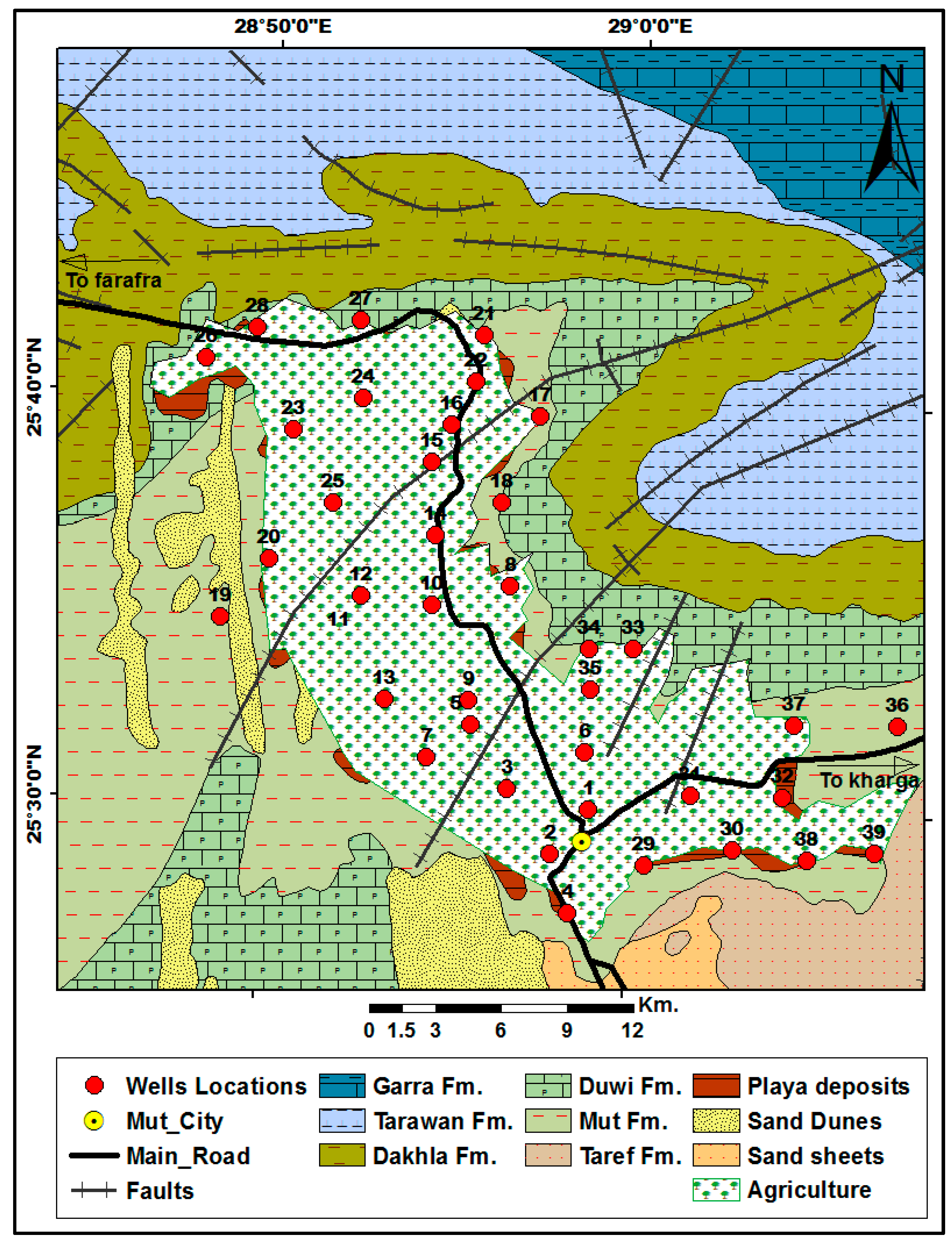
2. Study Area Description

The study area is located in Dakhla Oasis, Western Desert, Egypt, at longitudes 28°45′46.92″ and 29°09′35.76″ east, and between latitudes 25°25′07.51″ and 25°48′09.64″ north. Groundwater is the main source of water in the region, as it is used for various purposes through a number of wells dug in the region, whether municipal wells or private wells. Another source of water in the area is multiple agricultural drainage lakes interconnected by canals that provide water. Furthermore, there are scattered pockets of water dispersed among the farms. (Figure 1). These lakes result from over-irrigation, where horizontal leakage of irrigation water (flood irrigation) occurs from higher to lower areas through canals or lateral infiltration. This phenomenon wastes considerable amounts of water and causes subsequent salinization over time, rendering these resources unsuitable for any purpose. This ecosystem’s imbalance greatly impacts the quality and quantity of water [13,28,29,30]. The study area belongs to the hyper-arid part of Egypt [31] and is characterized by very dry climatic conditions, with intense sunlight. The study area belongs to the rainless part of Egypt. The hottest months are July and August, with a mean maximum temperature of 41.7 °C, and January and February are the coldest months, with a mean minimum temperature of 4.5 °C. Precipitation averages about 0.07 mm/year, comprising scarce summer rains and short spotty torrential winter rains. The relative humidity ranges between 17% in June and 35% in January, and the evaporation rate ranges between 8.8 mm/day in January and 37.6 mm/day in July, with an annual average of 24.3 mm (Egyptian Meteorological Authority, [32]). The Egyptian Meteorological Authority (EMA) primarily uses methods based on the FAO Penman–Monteith equation to calculate evaporation rates, relying on meteorological data such as temperature, relative humidity, wind speed, and solar radiation, which are then used in the FAO’s software tool (FAO 3.2) for calculations.

In environmental and agricultural studies, the Penman–Monteith equation is widely used to estimate evapotranspiration (ET). The standard form of the equation as recommended by the FAO (Food and Agriculture Organization) is:

$$ET={\displaystyle \frac{\left[0.408\mathsf{\Delta }\right(\mathrm{R}\mathrm{ₙ}-\mathrm{G})+\mathsf{\gamma }900/(\mathrm{T}+273)\mathrm{u}₂(\mathrm{e}\mathrm{ₛ}-\mathrm{e}\mathrm{ₐ}\left)\right]}{\mathsf{\Delta }+\mathsf{\gamma }(1+0.34 \mathrm{u}₂)}}$$

where ET is the evaporation rate (mm/day), Δ is the slope of the vapor pressure curve (kPa/°C), R_n is the net radiation at the crop surface (MJ/m²/day), G is the heat flux in the soil (MJ/m²/day), γ is the psychrophilic constant (kPa/°C), T is the air temperature at 2 m (°C), U₂ is the wind speed at 2 m (m/s), e_s is the saturated vapor pressure (kPa), and e_a is the actual vapor pressure (kPa).

The primary topographic feature of the Dakhla Oasis in terms of geomorphology is the steep scarp, which borders the oasis’s northern depression; it stretches more than 250 km in a WNW-ESE orientation and is irregular in its outline [31,33]. The escarpment consists of topographical features like recurring hills and terraces, featuring Upper Cretaceous to Paleocene shale and mudstone. It is typically topped with limestone and chalky limestone, reaching a height of 81 m in Mut and gradually decreasing northwestward to under 30 m near Al Qasr. In the study area, the Mut and Al-Qasr regions represent a depression of the vast lowlands that contain various geological formations that are considered among the factors that change the chemical composition of the water that is found between their pores or passing through them, thus affecting its quality.

Geology and Hydro-Geology

The geological formations are among the factors that determine the chemical nature of the water that is found between their pores or passing through them, and thus affecting its quality [28,29,30]. The geological and hydro-geological descriptions of the current study area are fully described in the previous study by Darwish et al. [13], and are shown in Figure 2. Briefly, these rock units in the study area date from the Late Cretaceous to Quaternary periods, and are represented from the base to the top by Maghrabi, Taref, Mut, Duwi, Dakhla, Tarawan, and Garra formations, and Quaternary deposits (Figure 2). The Maghrabi formation is primarily composed of marine shale and claystone. The Taref formation consists mainly of fine to medium-grained, well-sorted sandstone, with occasional shale interbeds. The Mut formation (also known as the Quseir Formation) forms the floor of the El-Dakhla depression [34] and includes variegated shale, siltstone, flaggy sandstone, ferruginous reddish claystone, and plant remains. The thickness of this formation decreases towards the east and south, where the Taref formation is exposed and extensively covers the study area’s surface. The Dawi formation, also known as the phosphate formation, comprises phosphate-bearing units alternating with black shale and limestone [35]. The Dakhla formation consists of dark grey shale, marl, and clay, interspersed with calcareous sandy and silty beds along the scarp face, and extends across parts of the plain west of Dakhla. The total thickness at the type section north of Mut town is approximately 230 m [36]. The Tarawan Formation is composed of fossiliferous, partly marly or chalky, yellowish-white limestone that grades into limestone, impure limestone, or dolomite [35]. The Garra formation is marked by white, thick-bedded, and chalky limestone beds at its top [37]. Quaternary deposits are characterized by significant aeolian accumulations, including frequent sand dunes and sand sheets, along with lacustrine playa deposits composed of horizontal alternating bands of friable sand, clay, and silt with plant remains. These deposits sometimes include intercalated salt crusts [38].

From a hydro-geological perspective, the Nubian Sandstone Aquifer System is a confined groundwater aquifer lying above impermeable rock that serves as the lower confining layer. The upper confining layer consists of impermeable variegated shale and clay overlaying the Nubian Sandstone Aquifer. The region’s main water-bearing sediments, derived from the Nubian sandstone succession, average 1500 m in thickness and are divided into three main subsurface water-bearing layers, separated by three alternating clay layers [39]. The Taref formation, with an average thickness of 110 m, represents the shallow water-bearing sediments. Water levels in this formation range from 60 to 120 m below the ground surface, with salinity levels ranging from 133 to 909 mg/L. The static water table of wells varies between 4.9 and 13.4 m, with an average total discharge of 895,608 m³ per day.

3. Materials and Methods

Samples were obtained from thirty-nine groundwater wells following a 10 min pumping process to eliminate stagnant water. One-liter polyethylene bottles, thoroughly rinsed with groundwater prior to sampling, were utilized. The bottles were filled to capacity with water samples and stored under standard preservation conditions. Furthermore, seven water samples from lakes and wastewater canals were gathered and preserved using an identical procedure; the samples were collected in January 2022. The 39 groundwater samples and 7 samples of wastewater from lakes and wastewater canals were sent to the Center Laboratories of the Ministry of Water Resources and Irrigation, New Valley, Egypt. The Global Positioning System (GPS) was employed to ascertain the location and elevation of the wells. In the field, electric conductivity (EC), total dissolved solids (TDS), temperature, and pH were measured. All the parameters in this study were measured according to the standard methods for examination of water and wastewater. The pH was measured with a pH meter (HANNA, HI98100) [40], while a handheld EC/TDS (HANNA, HI98311) was used to measure TDS, EC, and temperature. K⁺ and Na⁺ were determined using a flame photometer. Heavy metal concentrations were measured by flame atomic absorption spectrometry (AAS) [41]. Chloride and SO₄²⁻ were determined according to the standard methods [41]. The Versenate Titration method (EDTA) was used to determine the amount of soluble calcium and magnesium [41]. The total hardness (TH) was determined according to [42]. ArcGIS 10.3 and the Natural Neighbor interpolation method within the Spatial Analyst toolbox (The Spatial Analyst Toolbox is part of ArcGIS, a geographic information system software developed by Environmental Systems Research Institute, Redlands, California, USA), were used to generate the research area’s site map, sample sites, and all the spatial distribution maps of chemical parameters, pH, EC, TDS, total hardness, Na⁺, K⁺, Ca⁺², Mg⁺², Fe⁺², Mn⁺², Cl⁻, and SO₄⁻². By applying this technique, we visualized the spatial distribution of these parameters, identifying areas with high and low concentrations. The resulting maps provided valuable insights into potential spatial patterns and the factors influencing the distribution of these chemical constituents.

4. Results and Discussions

4.1. Physical Characteristics of Water

The results of physicochemical properties of water and wastewater are shown in

Table 1. Chemical analysis of the water samples.

		Groundwater Samples				Wastewater Samples
Parameter		Minimum	Maximum	Mean	STDEV	Minimum	Maximum	Mean	STDEV
pH		5.7	7.7	6.8	0.53	7	8.3	7.5	0.45
EC (µS/cm)		168	866.7	276	126.4	6766	114,000	40,526	39,481
TH	(mg/L)	41.5	129.6	73.6	27.77	467.4	13,482	4676	4358
TDS		101	520	165	75.8	6343	72,960	30,080	26,833
Ca+2		6.6	34.1	15.8	8.56	84.9	2400	813	782
Mg+2		3.4	12	8.2	2.02	62	1840	658	590.5
Na+		6	120	21.2	18.92	1023	28,538	8588	10,004
K+		4	20	11.4	4.81	55	1505	456	527.1
HCO3−		15	74	42.5	13.1	40	3752	972	1351.8
Cl−		19.2	94.7	38.1	18.19	929	43,693	12,293	15,326
SO4−2		7.5	103.5	35.4	19.8	15	12,935	3388	4634.7
Fe+2		1.4	10.6	4.7	2.43	0.01	0.15	0.06	0.06
Mn+2		0.02	4	0.5	0.87	0.07	0.9	0.35	0.323

and Figure 3 and Figure 4. Most of the collected groundwater samples from the study area have normal physical properties. The physicochemical results of the 39 groundwater samples and 7 samples from wastewater lakes and canals are presented in Supplementary Data, Tables S1 and S2. The data for this study were collected in January 2022, so all interpretations, analyses, and water assessments in the study area are specific to that date.

4.1.1. Temperature

In general, the temperature of the water varies greatly with the physiographical conditions. Ionic strength, conductivity, dissolution, solubility, and corrosion are all impacted by water temperature. The Dakhla Oasis’s groundwater in the study area is primarily fresh, with varying depths resulting in temperatures between 27 and 38 °C.

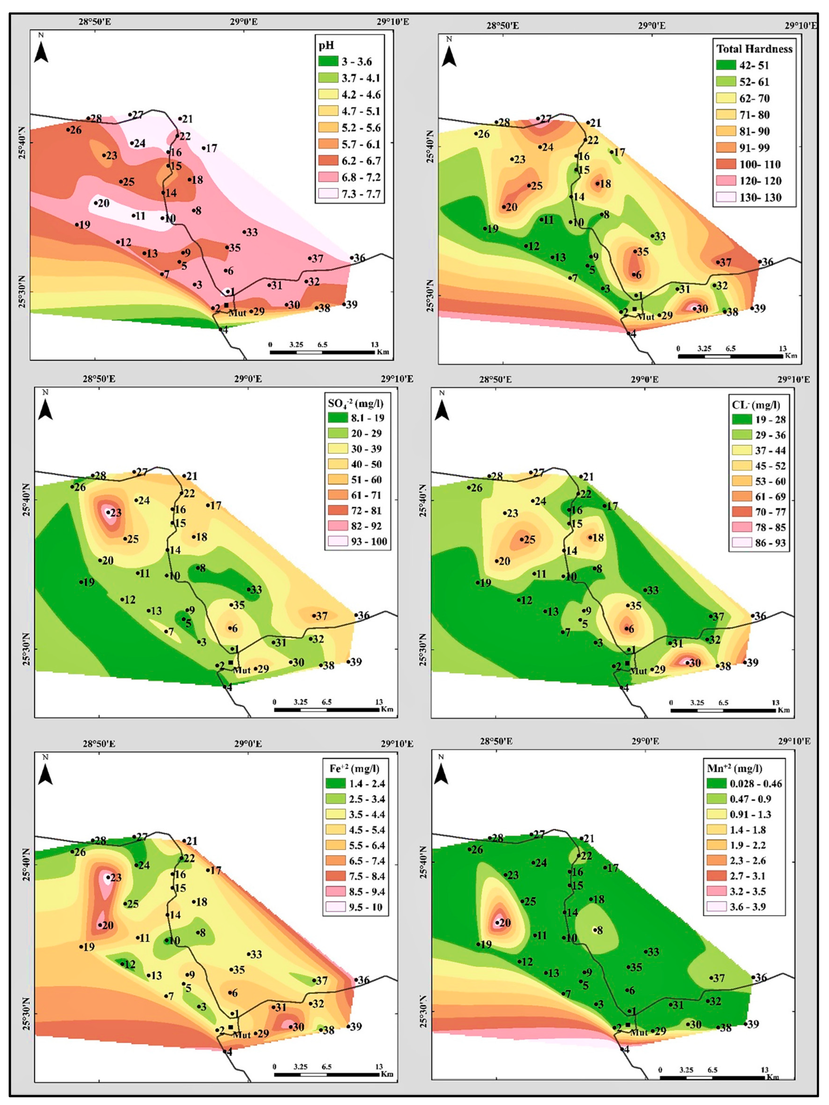
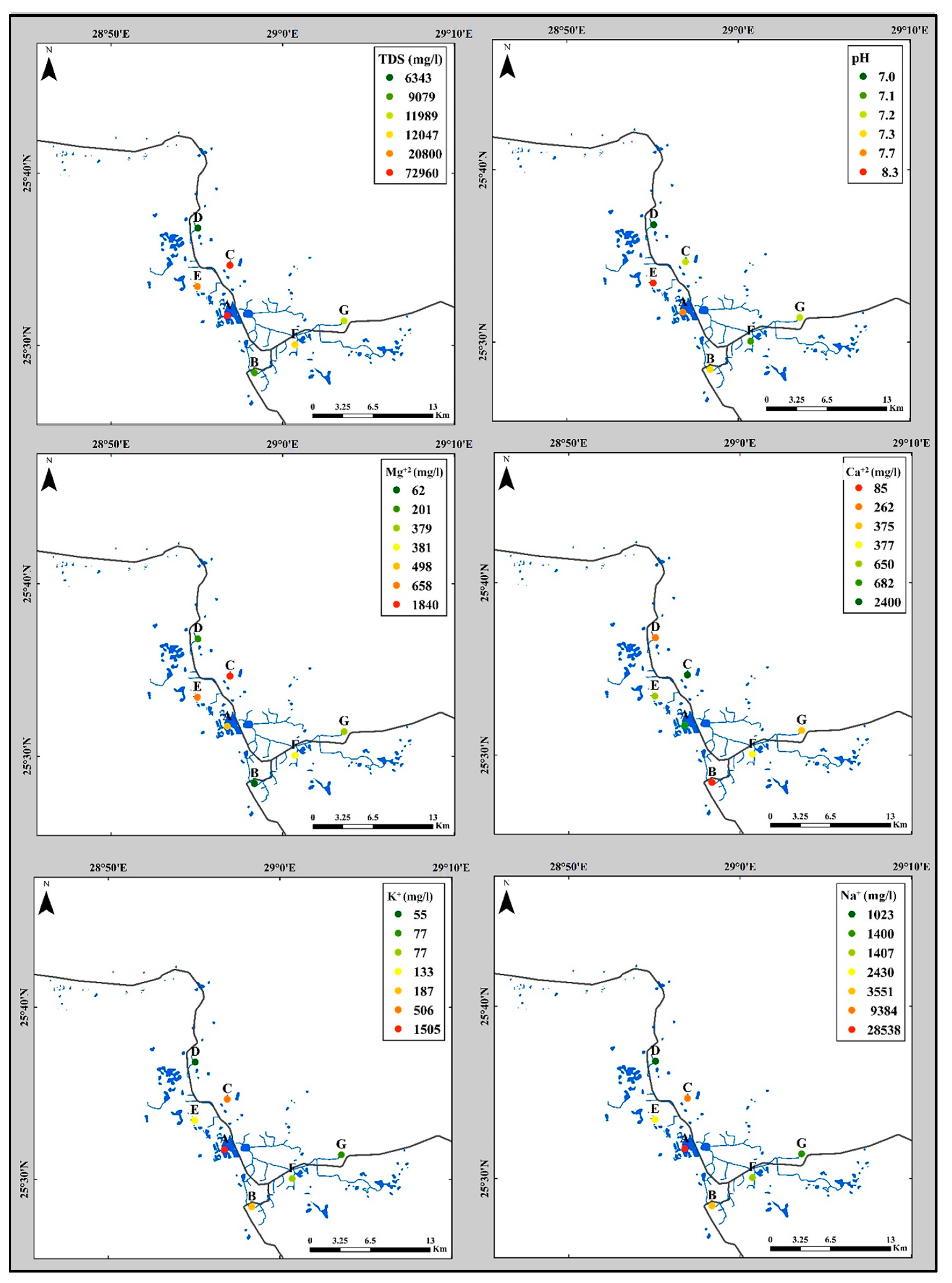
4.1.2. Hydrogen Ion Concentration (pH)

When water is indirectly exposed to the atmosphere, its pH generally ranges from 7.0 to just above 8.0, reflecting typical natural water conditions. The lower pH values can be attributed, to some extent, to the impact of agricultural fertilizers such as ammonium sulfate and superphosphate [43]. However, the pH value is a function of CO₂⁻, CO₃⁻, and HCO₃⁻, an equilibrium that is easily disturbed by the changes of CO₂ content. The pH in the study area ranges from 5.6 to 7.7, which reflects natural groundwater, and samples numbers 15, 23, and 38 have pH values of 5.8, 5.7, and 5.9, respectively, which indicates slightly acidic groundwater, In the wastewater lakes, the pH ranges from 7.0 to 8.3, which reflects a neutral to slightly alkaline water. The frequency distribution of the pH in the study area is shown in Figure 5 and Figure 6.

4.2. Chemical Characteristics of Water

The degree of diagnosis, the temperature of the water, and the chemical and physical characteristics of the nearby rocks all affect how much the chemical characteristics change. In the study area, the water’s chemical makeup is influenced by natural factors like soil and sediment with water content, as well as human-related factors such as sewage and agricultural runoff.

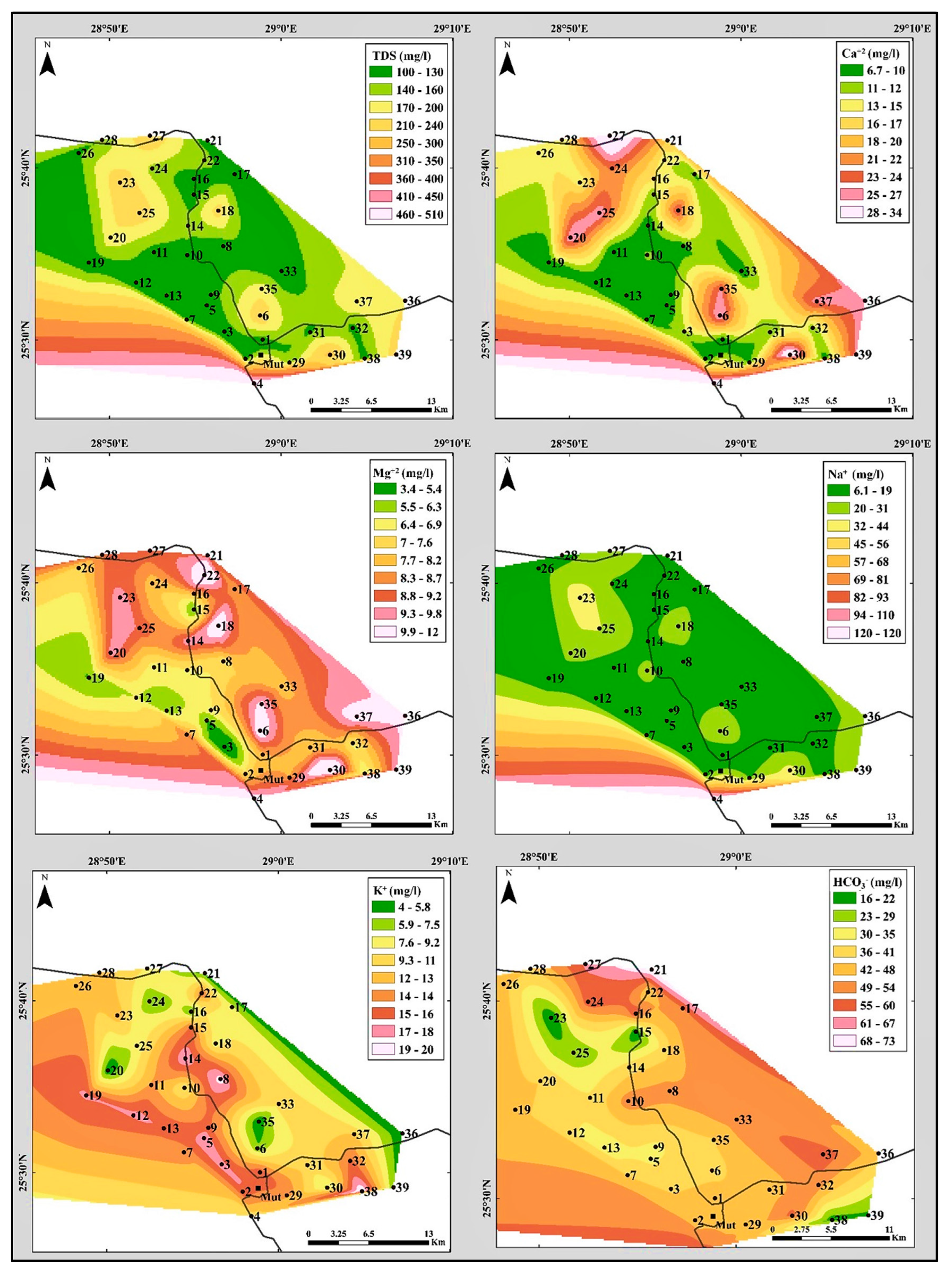
4.2.1. Total Dissolved Solids (TDS)

The analysis of TDS for all samples showed values less than 500 mg/L, which indicate significant differences in TDS from one sample to another [44,45]. Water is classified into four categories according to its salinity. TDS in the study area ranged from 101 to 520 mg/L with a mean concentration of 165 mg/L. According to [46,47], the groundwater in the current study is fresh and suitable for drinking, while TDS of the wastewater ranges from 6343 to 72,960 mg/L, with a mean concentration of 30,080 mg/L. Based on the classification suggested by [46,47], the wastewater samples are moderately saline water (brackish) to briny water (

Table 2. Water types according to their TDS of the study area.

Hem [47]		Davis and Dewiest [46]		Present Study
Water Type	TDS (mg/L)	Water Type	TDS (mg/L)	Groundwater	Wastewater
Freshwater	<1000	Freshwater	<1000	100% of the samples	---------
Moderately saline water	3000–10,000	Brackish	1000–10,000	-----------	(B and D samples)
Very saline water	10,000–35,000	Salty	10,000–100,000	-----------	(E–F–G samples)
Briny water	>35,000	brine	>100,000	-----------	(A and C samples)

). This high content of TDS is because of the discharge of different pollutants, such as human and animal sewage, where sewage water is poured into these ponds. Additionally, the evaporation, especially in the summer, increases the TDS in these lakes. In general, TDS in the current study increases in southwest directions. The frequency distribution of the TDS in the study area is shown in Figure 6 and Figure 7.

4.2.2. Total Hardness (TH)

Usually, the concentration of CaCO₃ in (ppm) present in the water is expressed as water hardness. Multivalent cations, particularly calcium and magnesium, are often present in significant concentrations in the natural waters. Water for domestic uses should not contain more than 80 mg/L total hardness. Water from aquifers with limestone or gypsum may contain 200 to 300 mg/L hardness or more; soft water easily contains a few minerals and lathers, but hard water is rich in minerals, causing “scale” in kettles.

There are two types of hardness in water, carbonate and non-carbonate. Hardness (temporary hardness) or carbonate hardness includes calcium and magnesium, which can combine with bicarbonate. Non-carbonate hardness, also known as permanent hardness, arises from the amalgamation of calcium and magnesium with sulfate, chloride, and nitrate ions, supplemented by minor constituents that contribute to its overall hardness. According to Hem [48], the hardness associated with carbonate compounds is quantified in terms of the calcium carbonate equivalent:

H_r = Ca⁺² × CaCO₃/Ca⁺² + Mg⁺² × CaCO₃/Mg⁺²

where H_r is the hardness, Ca⁺² and Mg⁺² are measured in ppm, and the ratios in the formula are weights. Carbonate hardness can be calculated by adding the milliequivalents of Ca⁺² and Mg⁺² per liter and multiplying the sum by 50. The non-carbonate hardness can be calculated as the difference between carbonate hardness and the alkalinity of the water as CaCO₃ (if hardness as CaCO₃ exceeds the alkalinity as CaCO₃). The alkalinity is expressed as the equivalent concentration of CaCO₃ obtained by adding the equivalents of CaCO₃ and HCO₃⁻ and expressing the sum as mg/L of CaCO₃. Water is classified regarding its hardness into four classes (

Table 3. Water classes according to their total hardness [23,24,25,26,27,28,29,30,31,32,33].

Class	Total Hardness (mg/L)	Present Study
		Groundwater	Wastewater
Soft	0–60	21 samples (53.85%)	------------
Moderately hard	61–120	16 samples (41.02%)	------------
Hard	121–180	2 samples (5.13%)	------------
Very hard	>180	------------	All samples (100%)

).

In the current study, the carbonate hardness in our samples ranges between 41.53 and 129.60 mg/L, with an average concentration of 73.6 mg/L. Thus, most of the groundwater samples are considered to be in the soft to moderately hard classes, and only two samples are hard (samples 27 and 30). The high value for TH may be due to alkaline soil, containing elements such as calcium and magnesium [49]. The wastewater is considered to be a very hard class, where the total hardness ranges between 467.4 and 13,482 mg/L, with an average concentration of 4676 mg/L. The frequency distribution of the water hardness in the study area is shown in Figure 5 and Figure 8.

4.2.3. Electrical Conductivity (EC)

When water has a high EC value, it will be toxic to different plants [50]. Agriculture crop productivity depends on EC, which is the most important water quality guideline [51].

Recently, Darwish et al. [13] found that the electrical conductivity (EC) values in groundwater from Dakhla Oasis varied between 168 and 866.7 µS/cm, averaging 276 µS/cm. The elevated EC levels observed in specific groundwater samples suggest the presence of certain salts in the water. Additionally, wastewater EC values ranged from 6766 to 114,000 µS/cm, with an average concentration of 40,526 µS/cm. The EC values in the groundwater samples indicate excellent water quality suitable for irrigation purposes, whereas the wastewater samples exhibit a water class ranging from poor to good [26].

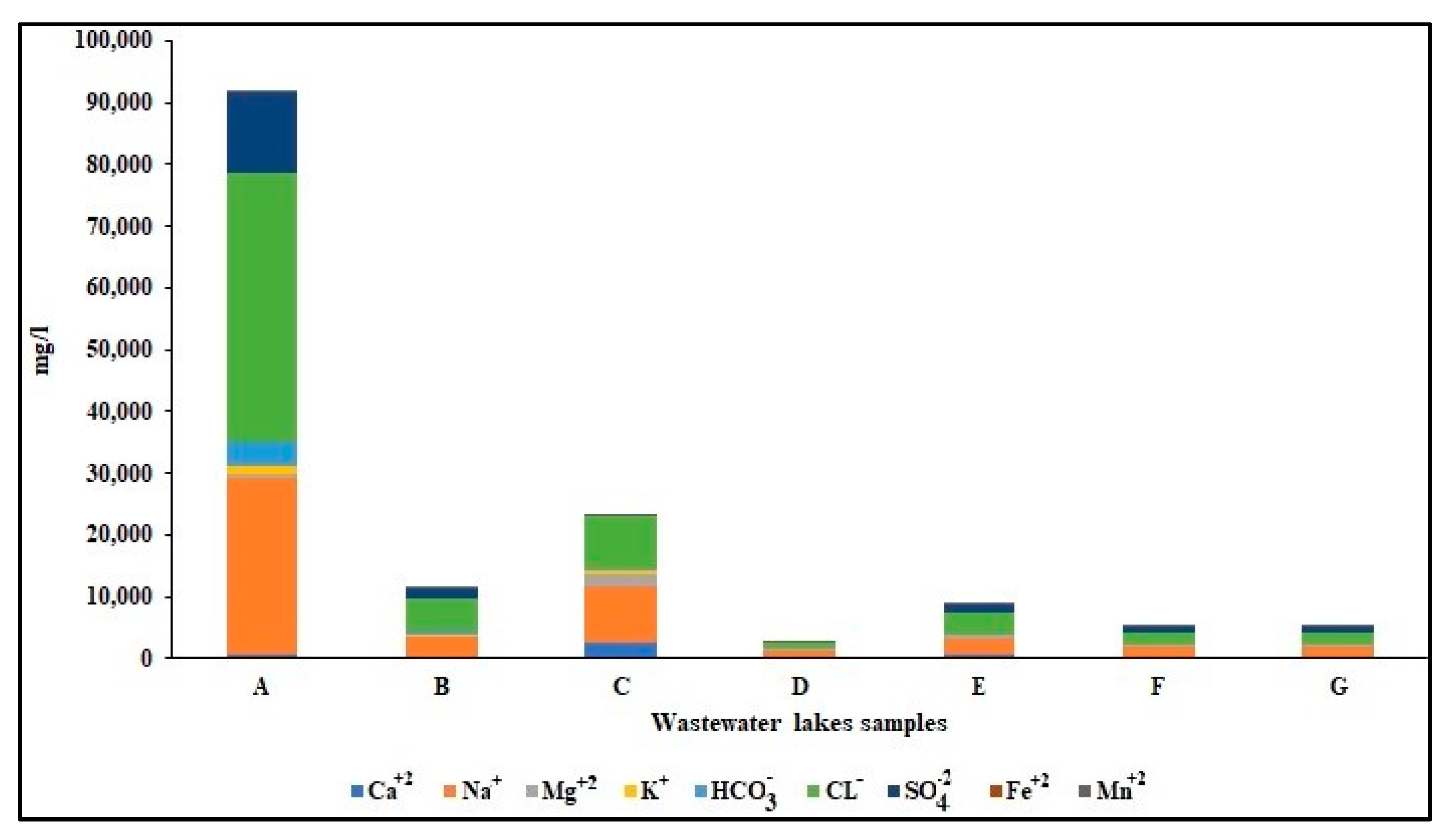
4.2.4. Ion Concentrations and Distribution

The primary source of elements in the groundwater is precipitation. The water in the study area comes from the Nubian Sandstone Aquifer System (NSAS), the largest known groundwater aquifer in the world, spanning four countries in northeastern Africa: northwestern Sudan, northeastern Chad, southeastern Libya, and most of Egypt [13]. Known as a fossil aquifer, the NSAS is composed of solid iron-rich sandstone with significant layers of oil shale and clay, as noted in the region’s geological profile. The aquifer’s water is typically fresh to slightly saline, with sodium as the dominant cation, surpassing calcium and magnesium, while chloride prevails over sulfates and bicarbonates [39]. The concentrations of these elements are a direct result of the aquifer’s water-bearing layers. High levels of sodium, chloride, and sulfates indicate filtration and dissolution processes of gypsum rocks and clay, influenced by the aquifer’s vast expanse and the ancient age of the water, which dates back to the Paleozoic through Upper Cretaceous periods. These factors allow rock elements to dissolve into the water over time [39].

Surface water in the study area, represented by agricultural drainage ponds, largely originates from groundwater, with some contributions from sewage water, such as in Mut Lake. The chemical element concentrations in this surface water are significantly higher than in groundwater due to environmental factors, climatic conditions, human activities, and the area’s geological formations. These lakes formed naturally from excess irrigation water flowing into lower-lying areas, where it dissolves minerals and increases the concentration of chemical elements. The addition of sewage water further raises the concentration of specific elements like chloride. In the case of Mut Lake, due to a mixture of agricultural runoff and sewage, the high chloride levels are linked to both human activities and animal waste. The arid climate and high evaporation rates also amplify the concentration of these elements, making them more prevalent than their source in the groundwater.

• A. Major Ions:

The distribution of the major ions in the study area in the groundwater and wastewater are shown in Figure 5, Figure 6, Figure 7 and Figure 8, and discussed in the following:

• Calcium and magnesium ion concentrations and distribution:

The two minerals that cause water hardness are calcium and magnesium dissolved in water [51]. Ca²⁺ is one of the main cations present in surface and groundwater. Calcium is present in sedimentary rocks in carbonates, like limestone and dolomite, and in sulfates, like gypsum and anhydrite. Since gypsum is relatively soluble in water, water contains large amounts of calcium when it comes into contact with gypsum. Water can dissolve up to 600 mg/L of Ca²⁺ at room temperature from gypsum [48]. Ca²⁺ concentrations in drinking water are usually less than 100 mg/L but brines contain up to 7500 mg/L. In subsurface waters, calcium is a frequent ion because of its abundance in the crust of the Earth and its mobility in the hydrosphere [46]. In our study, Ca²⁺ content in the well samples ranged between 6.6 mg/L (sample No. 11) and 34.1 mg/L (sample No. 27), below the suitable limit of 75 mg/L (WHO [52]), while in wastewater lakes and canals, Ca²⁺ content ranged from 84.87 mg/L (sample No. B) to 2400 mg/L (sample No. C), and was above the acceptable limit of 75 mg/L (WHO [52]).

Magnesium is similar to Ca²⁺ as a principal cation in the groundwater and surface water, and as a major cause of water hardness. Occasionally, magnesium is mixed with calcium carbonate and clay minerals in sedimentary rocks to form magnesite and other carbonates. Magnesium and calcium are in equal amounts in the case of dolomite. The concentration of Mg²⁺ in drinking water is usually less than 50 mg/L, but in ocean water is about 1000 mg/L and reaches 57,000 mg/L in brines. If it is present in a high concentration, it will have laxative effects. In the current study, Mg²⁺ content in groundwater well samples ranged between 3.36 mg/L (sample No. 3) and 11.18 mg/L (sample No. 18), and was below the acceptable limit of 30 mg/L (WHO [52]), while in wastewater lakes and canals, the Mg²⁺ ranged between 61.97 mg/L (sample No. B) and 1840 mg/L (sample No. C), and was higher than the acceptable limit of 30 mg/L (WHO [52]).

• Sodium and potassium ions concentrations and distribution:

Natural water typically contains a notable amount of sodium, with shale and clay sediments frequently contributing to elevated sodium levels. Additional sources include the leaching of sodium-rich evaporates like halite [13,43,48]. The concentration of sodium in natural water typically falls below 200 mg/L, contrasting with seawater at around 10,000 mg/L and brines at approximately 25,000 mg/L [13,43,48]. K⁺ concentration in the groundwater is usually less than sodium concentrations. Clay minerals are the main natural source of K⁺ in sedimentary rocks. K⁺ concentration is usually under 10 mg/L in natural water, but up to 100 mg/L in hot springs and 25,000 mg/L in brines [13,43,48]. In the study area, sodium content ranged between 6 mg/L (sample No.33) and 120 mg/L (sample No. 4), and was below the acceptable limit of 200 mg/L (WHO [52]), and potassium content ranged between 4 mg/L (samples No. 20, 35, and 36) and 20 mg/L (sample No. 38), and was below the acceptable limit of 12 mg/L (WHO [52]). In wastewater lakes, the sodium content ranged between 1023 mg/L (sample No. D) and 28,538 mg/L (sample No. A), and potassium content ranged between 55 mg/L (sample No. D) and 1505 mg/L (sample No. A). High concentrations of K⁺ may lead to Mg²⁺ deficiency and iron chlorosis. An imbalance of Mg²⁺ and K⁺ may be toxic, but the high calcium levels reduce the effects of both Mg²⁺ and K⁺ [53].

• Bicarbonate ions concentration and distribution:

The common concentration of bicarbonate in groundwater is 200 mg/L, and higher concentrations of bicarbonate can occur where CO₂ is produced within the aquifer. In our study, the bicarbonate concentrations in groundwater range between 15.1 mg/L (sample No. 15) and 58.6 mg/L (sample No. 24), and are below the acceptable limit of 500 mg/L (WHO [52]), while in wastewater lakes and canals, the bicarbonate content ranges between 39.9 mg/L (sample No. D) and 3752 mg/L (sample No. A).

• Sulphate ions concentrations and distribution:

In natural aquatic environments, sulphate derived from gypsum and anhydrite holds significant importance. Typically, the sulphate concentration in regular water remains below 300 mg/L, except in wells affected by acid mine drainage, where it can exceed this limit. In certain brines, sulphate levels may soar up to 200,000 mg/L. Within the investigated region, the sulphate concentrations in groundwater well samples varied from 7.5 mg/L (sample No. 8) to 103.5 mg/L (sample No. 23), all falling below the acceptable limit of 250 mg/L as per WHO standards [52]. Conversely, in the wastewater lake, sulphate content ranged from 14.6 mg/L (sample No. D) to 12,935 mg/L (sample No. A).

• Chloride ions concentrations and distribution:

Chloride ions exist in all drinking water, exhibiting an average of 3 mg/L in rainwater and soaring to 19,000 mg/L in seawater [53]. Water containing less than 150 mg/L of chloride is considered suitable for a wide range of purposes. In the study area, chloride concentrations in groundwater range between 19.23 mg/L (sample No. 33) and 94.7 mg/L (well no.30), and were within the acceptable limit of 250 mg/L (WHO [52]), while in wastewater lake the chloride content ranges between 928.6 mg/L (sample No. D) and 43,693 mg/L (sample No. A), and was above the acceptable limit of 250 mg/L (WHO [52]).

• B. Trace elements:

Some trace elements, such as Fe⁺², Mn⁺² Ni⁺², and Pb⁺², are measured in some water points in the study area. The distributions of the trace elements in the groundwater and wastewater in the study area are shown in Figure 6 and Figure 9.

• Iron (Fe⁺²) and Manganese (Mn⁺²)

The metallic taste in groundwater is mainly because of the presence of iron and manganese. Iron and manganese may be removed by a water softener if they are present in low quantities. Aeration, chlorination, and feeding ozone or H₂O₂ can aid in the precipitation of Fe²⁺, which is removed from the water by filtration. Iron and manganese can also be removed with potassium permanganate feed combined with manganese greens and filters.

The prevalent form of iron in groundwater is Fe²⁺. In the presence of oxygen, Fe²⁺ becomes Fe³⁺, causing the water to discolor brown as Fe(OH)₃ precipitates. Moreover, the activity of heterotrophic and iron oxidizing bacteria activity could also increase or decrease the concentration of iron in groundwater. The existence of iron in drinking water results in a metallic flavor. As per the guidelines from the American Public Health Service, the highest acceptable concentration of iron in drinking water is 0.3 mg/L (U.S. Public Health Service 1962). Different types of microorganisms could have an effect on the chemistry of Fe²⁺/Fe³⁺ in groundwater [33]. River water contains a higher concentration of iron (about 0.67 mg/L) compared to sea water (0.003 mg/L) [9]. The average iron content estimated for water derived from sedimentary rocks are as follows: sandstone, 0.74 mg/L; loose sand average, 0.31 mg/L; siltstone and clay, 1.61 mg/L; and limestone and clay, 0.42 mg/L. In the current study, iron concentration in groundwater wells samples ranged from 1.4 mg/L (water samples No. 12 and 27) to 10.6 mg/L (water sample No. 23), which is higher than the permissible limit of 0.3 mg/L (WHO [52]). In wastewater lakes and canals, the iron content ranged between 0.01 mg/L (water sample No. D) and 0.15 mg/L (water sample No. A), which is considered below the permissible limit of 0.3 mg/L (WHO [52]).

In natural water, Mn²⁺ is normally less than 0.2 mg/L, while in groundwater it reaches more than 10 mg/L. The hydrated oxides of Mn²⁺ are much less soluble than those of Fe²⁺, although they are present in most groundwater at lower concentrations than Fe²⁺ [32,33]. The maximum concentration of Mn²⁺ for different water supplies is set at 0.05 mg/L, and the maximum limit is 0.5 mg/L according to the World Health Organization [16]. In the current study, Mn²⁺ in groundwater well samples averaged between 0.02 mg/L (water samples No. 27 and 35) and 4 (samples No. 4 and 20), and was over the acceptable limit of 0.1mg/L (WHO [52]). In wastewater lakes and canals, the manganese content ranged between 0.07 mg/L (water sample No. D) and 0.9 mg/L (water sample No. A), and was above the acceptable limit of 0.3 mg/L (WHO [52]).

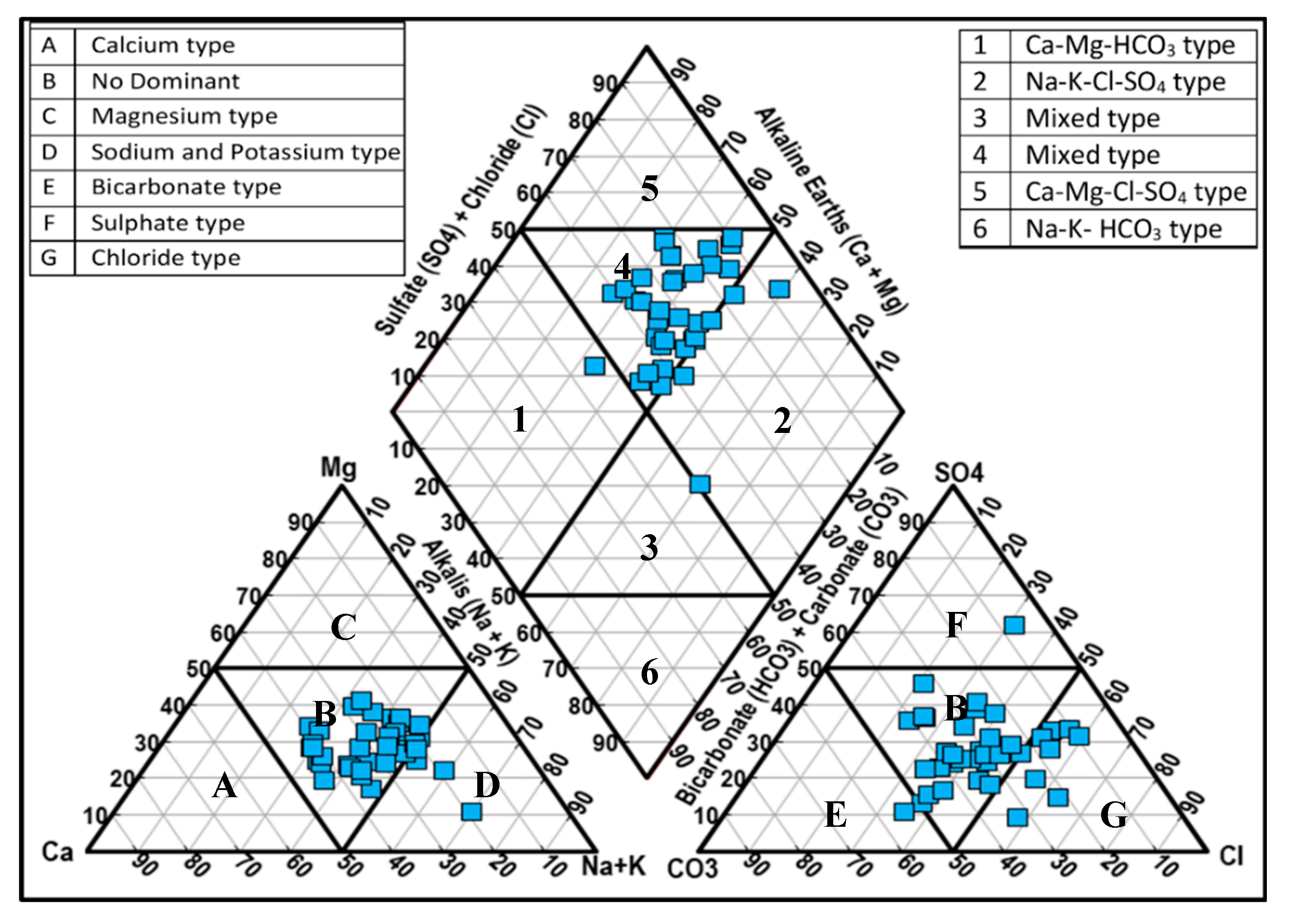
4.2.5. Hydro-Chemical Classifications

Both the trilinear diagram [54] and the semilogarithmic diagram [55] were used to correlate the chemical composition of the water in the area. Various water facies were recognized and distinguished using Piper’s diagram [56].

The trilinear diagram stands out as a commonly employed graphical technique for categorizing natural waters. It serves as a valuable instrument for interpreting water analysis. The categorization approach is based on the millionth percentage equivalents of both cations and anions. This procedure utilizes two triangular diagrams, with one on the left dedicated to plotting cations and another on the right for plotting anions, both within a diamond-shaped field. The diagram consists of two identical triangles. Broadly speaking, the upper triangle of this diamond-shaped field represents water with secondary salinity properties, indicating higher concentrations of sodium and chloride compared to sodium and potassium. Calcium and magnesium appear to have primary alkalinity properties in the lower triangle, whereas carbonate and bicarbonate do not. In the area of study, the data of the chemical analysis of the samples are separated into three groups according to their locations (Figure 10). The data representation showed that the samples are close to each other and could not be distinguished into groups, indicating that the groundwater there has a good connection and a close relationship. A majority of cations are sodium ions, while anions such as carbonate and bicarbonate are most dominant. On the other hand, the majority of the samples are of Na-Cl facies. In the cation’s triangle, Na⁺ and K⁺ are higher than Ca²⁺ and Mg²⁺, and in the anion triangle, carbonate and bicarbonate ions are higher than chloride ions, and sulfate ions are the lowest.

• Trilinear diagram:

The trilinear diagram was generated through the utilization of the Excel software program in 2022. In the upper triangle of the diagram, water samples exhibit secondary salinity properties characterized by higher levels of sulfate and chloride in comparison to sodium and potassium. On the other hand, the lower triangle showcases calcium and magnesium, which are deemed to possess primary alkalinity properties when contrasted with the carbonates and bicarbonates found in the upper triangle. The findings from the analyzed samples were graphically represented on a Piper diagram.

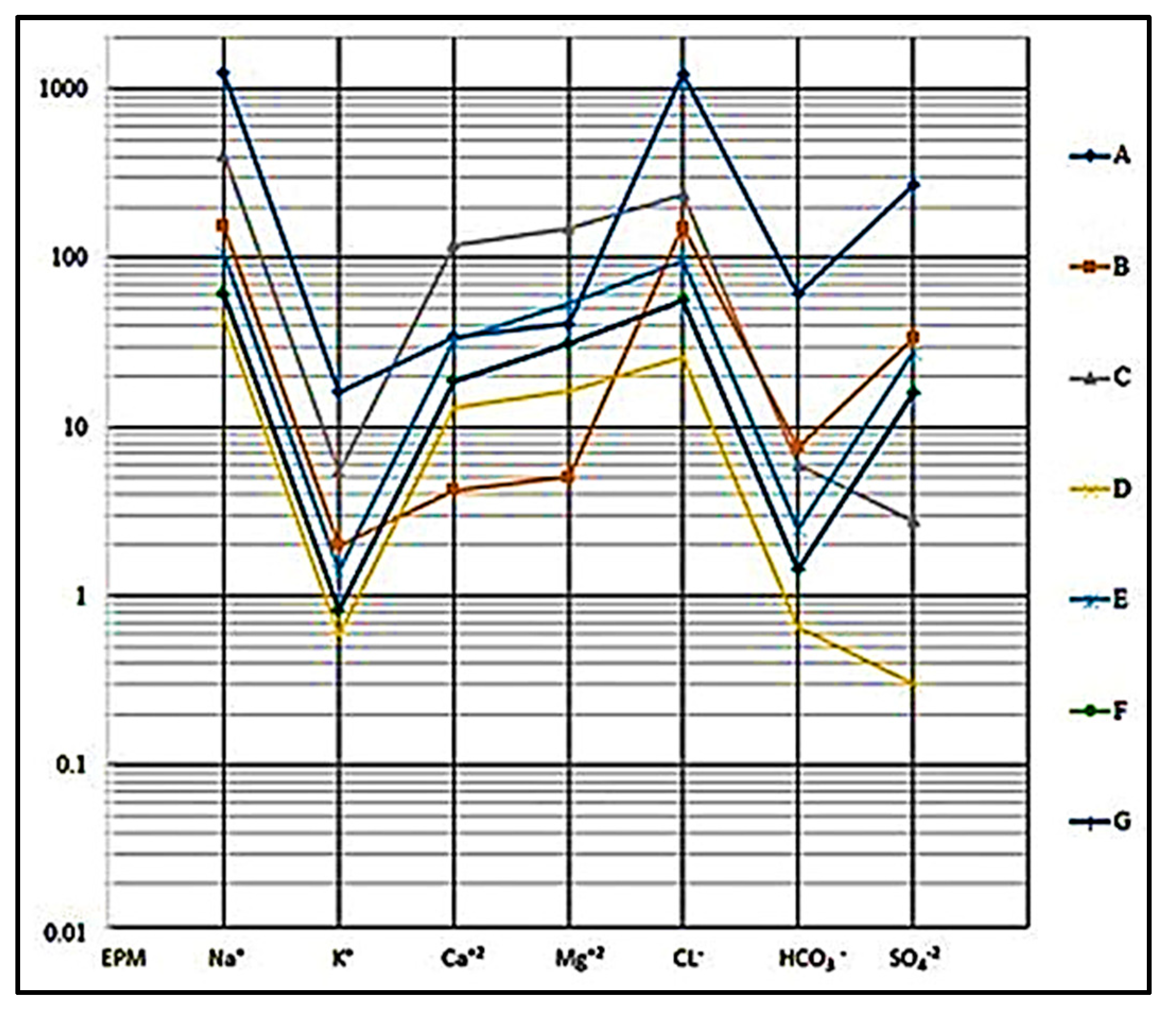
• Semilogarithmic diagram:

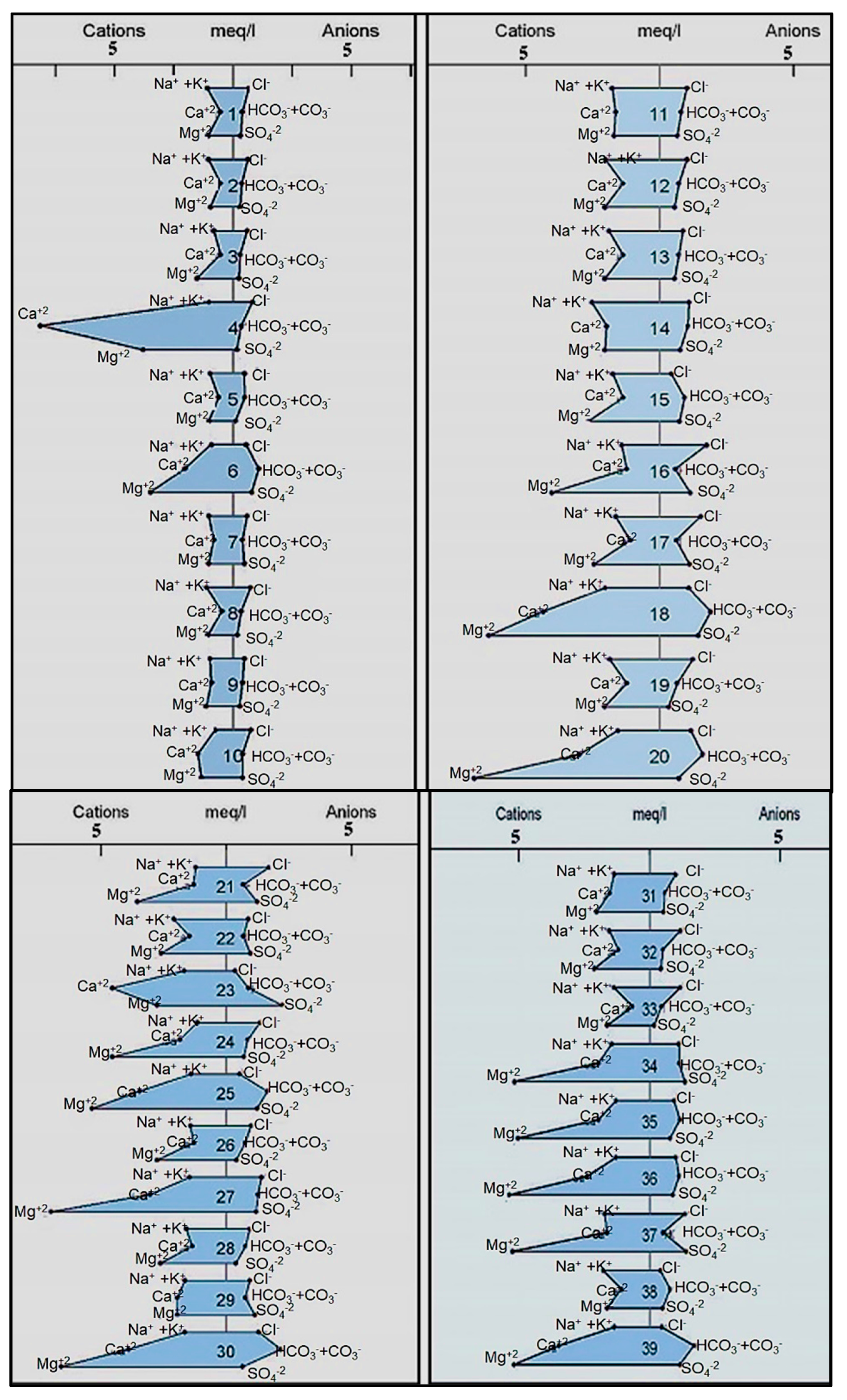
The Schoeller semi-logarithmic diagram was created using the Excel software program (2016); the analysis results are plotted on the Schoeller diagram [55]. This diagram can be used to represent an analysis by connecting points related to gravimetric concentrations. Logarithmic scales are used to express concentration values. The plotting of data on a diagram of this type may be helpful in comparative analysis of the major ions; in particular, for water samples that are high in this diagram (Figure 11 and Figure 12), it is clear that Na⁺ > Cl⁻ > Ca⁺² >SO₄⁻² > HCO₃⁻ > Mg⁺² > K⁺. Analyses of the chemical composition of the water samples are plotted in equivalents per million (meq/L). According to the Schoeller diagram, the general patterns in the samples were HCO₃⁻ > Cl⁻ > SO₄⁻² > Na⁺ > Ca⁺² > K⁺ > Mg⁺², while in the wastewater samples they were Cl⁻ > Na⁺ > SO₄⁻² > HCO₃⁻ > Ca⁺² > Mg⁺² > K⁺.

• Stiff diagram

Stiff Jr. [57] developed a graph to represent the chemical analysis called the Stiff diagram. It is widely used to display the major ion content in water samples. The diagram has a polygonal shape (four parallel horizontal axes extending on either side of a vertical zero axis). Major ions (meq/L) and anions are plotted on the right, while cations are plotted on the left of the zero axis. A Stiff diagram can be used to compare water from different sources and can be used to visualize ionic-related water bodies in order to determine their flow paths, or to show how the ionic composition of a water body changes over time. The plotted points yield a pattern with the shape characteristics of the composition of the representative sample. The analysis generates polygons that highlight similarities or differences in overall water chemistry. The width of each polygon serves as an approximate representation of the total ionic content.

The results revealed that the proximity of groundwater samples is characterized by the abundance of sodium, potassium, and magnesium cations and chloride anions. Lake samples were characterized by the abundance of sodium and potassium cations and chloride anions (Figure 13 and Figure 14).

4.2.6. Water Type

According to the results obtained from the chemical analysis, the Piper, Schoeller, and Stiff diagrams, and the ion dominance in the water samples, the groundwater types are differentiated depending on their localities, and the abundance sequence for both anions and cations following the variety orders are distinguished (

Table 4. Groundwater types in the study area.

Sample	(%)			(%)			Water Type
No.	Na+ & K+	Ca+2	Mg+2	CL−	HCO3−	SO4−2
1	41	23	36	38	38	24	Na+ > Mg+2 > Ca+2	Sodium -Chloride
							CL− > HCO3− > SO4−2
2	44	22	34	38	38	24	Na+ > Mg+2 > Ca+2	Sodium -Chloride
							CL− > HCO3− > SO4−2
3	47	36	17	36	41	23	Na+ > Ca+2 > Mg+2	Sodium -Bicarbonate
							HCO3− > CL− > SO4−2
4	70	19	11	37	50	13	Na+ > Ca+2 > Mg+2	Sodium -Bicarbonate
							HCO3− > CL− > SO4−2
5	30	24	26	58	33	9	Na+ > Mg+2 > Ca+2	Sodium -Chloride
							CL− > HCO3− > SO4−2
6	39	37	24	54	16	30	Na+ > Ca+2 > Mg+2	Sodium -Chloride
							CL− > SO4−2 > HCO3−
7	44	20	37	35	31	34	Na+ > Mg+2 > Ca+2	Sodium -Chloride
							CL− > SO4−2 > HCO3−
8	45	23	32	38	47	15	Na+ > Mg+2 > Ca+2	Sodium -Bicarbonate
							HCO3− > CL− > SO4−2
9	50	22	28	45	31	24	Na+ > Mg+2 > Ca+2	Sodium -Chloride
							CL− > HCO3− > SO4−2
10	52	23	25	35	38	27	Na+ > Mg+2 > Ca+2	Sodium -Chloride
							CL− > SO4−2 > HCO3−
11	50	19	31	42	31	27	Na+ > Mg+2 > Ca+2	Sodium -Chloride
							CL− > HCO3− > SO4−2
12	49	22	29	41	34	25	Na+ > Mg+2 > Ca+2	Sodium -Chloride
							CL− > HCO3− > SO4−2
13	49	23	28	43	30	27	Na+ > Mg+2 > Ca+2	Sodium -Chloride
							CL− > HCO3− > SO4−2
14	48	17	35	46	28	26	Na+ > Mg+2 > Ca+2	Sodium -Chloride
							CL− > HCO3− > SO4−2
15	47	29	24	53	14	33	Na+ > Ca+2 > Mg+2	Sodium -Chloride
							CL− > SO4−2 > HCO3−
16	26	40	34	24	40	36	Na+ > Ca+2 > Mg+2	Sodium -Bicarbonate
							HCO3− > SO4−2 > CL−
17	21	28	39	26	37	37	Na+ > Mg+2 > Ca+2	Sodium -Bicarbonate
							HCO3− > SO4−2 > CL−
18	42	33	25	52	17	31	Na+ > Ca+2 > Mg+2	Sodium -Chloride
							CL− > SO4−2 > HCO3−
19	49	24	27	40	44	16	Na+ > Mg+2 > Ca+2	Sodium -Bicarbonate
							HCO3− > CL− > SO4−2
20	33	42	25	56	24	20	Na+ > Ca+2 > Mg+2	Sodium -Chloride
							CL− > HCO3− > SO4−2
21	29	38	33	26	37	37	Ca+2 > Mg+2 > Na+	Calcium -Bicarbonate
							HCO3− > SO4−2 > CL−
22	38	24	38	35	26	39	Na+ > Mg+2 > Ca+2	Sodium -Sulphate
							SO4−2 > CL− > HCO3−
23	59	19	22	31	7	62	Na+ > Mg+2 > Ca+2	Sodium -Sulphate
							SO4−2 > CL− > HCO3−
24	34	42	24	39	36	25	Ca+2 > Na+ > Mg+2	Calcium -Chloride
							CL− > HCO3− > SO4−2
25	44	36	20	56	11	33	Na+ > Ca+2 > Mg+2	Sodium -Chloride
							CL− > SO4−2 > HCO3−
26	40	32	28	46	35	19	Na+ > Ca+2 > Mg+2	Sodium -Chloride
							CL− > HCO3− > SO4−2
27	37	44	19	42	27	31	Ca+2 > Na+ > Mg+2	Sodium -Chloride
							CL− > SO4−2 > HCO3−
28	39	29	32	48	34	18	Na+ > Mg+2 > Ca+2	Sodium -Chloride
							CL− > HCO3− > SO4−2
29	50	21	29	34	25	41	Na+ > Mg+2 > Ca+2	Sodium -Chloride
							CL− > SO4−2 >HCO3−
30	40	37	23	63	22	15	Na+ > Ca+2 > Mg+2	Sodium -Chloride
							CL− > HCO3− > SO4−2
31	44	25	31	37	37	26	Na+ > Mg+2 > Ca+2	Sodium -Chloride
							CL− > HCO3− > SO4−2
32	45	26	29	33	45	22	Na+ > Mg+2 > Ca+2	Sodium -Bicarbonate
							HCO3− > CL− > SO4−2
33	34	25	41	35	54	11	Na+ > Mg+2 > Ca+2	Sodium -Bicarbonate
							HCO3− > CL− > SO4−2
34	29	41	30	40	23	37	Ca+2 > Mg+2 > Na+	Calcium -Chloride
							CL− > SO4−2 > HCO3−
35	30	42	28	50	23	27	Ca+2 > Na+ > Mg+2	Calcium -Chloride
							CL− > SO4−2 > HCO3−
36	33	41	26	47	24	29	Na+ > Ca+2 > Mg+2	Sodium -Bicarbonate
							HCO3− > SO4−2 > CL−
37	30	42	28	21	33	46	Ca+2 > Na+ > Mg+2	Calcium -Sulphate
							SO4−2 > HCO3− > CL−
38	51	21	28	55	16	29	Na+ > Mg+2 > Ca+2	Sodium -Chloride
							CL− > SO4−2 > HCO3−
39	43	35	22	59	9	32	Na+ > Ca+2 > Mg+2	Sodium -Chloride
							CL− > SO4−2 > HCO3−

). The study area is characterized by six main groundwater types, which are as follows:

• Na⁺ > Mg⁺²(Ca⁺²) > Ca⁺² (Mg⁺²) and Cl⁻ > SO₄⁻²(HCO₃⁻) > HCO₃⁻(SO₄⁻²), the groundwater type is sodium–chloride.
• Na⁺ > Mg⁺²(Ca⁺²) > Ca⁺²(Mg⁺²) and HCO₃⁻ > SO₄⁻²(Cl⁻) > Cl⁻(SO₄⁻²), the groundwater type is sodium–bicarbonate.
• Na⁺ > Mg⁺²(Ca⁺²) > Ca⁺²(Mg⁺²) and SO₄⁻² > HCO₃⁻(Cl⁻) > Cl⁻(HCO₃⁻), the groundwater type is sodium–sulphate.
• Ca⁺² > Na⁺(Mg⁺²) > Mg⁺²(Na⁺) and Cl⁻ > SO₄⁻²(HCO₃⁻) > HCO₃⁻(SO₄⁻²), the groundwater type is calcium–chloride.
• Ca⁺² > Na⁺(Mg⁺²) > Mg⁺²(Na⁺) and SO₄⁻² > HCO₃⁻ > Cl⁻, the groundwater is calcium–sulphate.
• Ca⁺² > Na⁺(Mg⁺²) > Mg⁺²(Na⁺) and HCO₃⁻ > SO₄⁻² > Cl⁻, the groundwater is calcium–bicarbonate.

According to the results obtained from the chemical analysis, and on the ion dominance in the wastewater of the current study, the abundance sequence for both anions and cations follows the order Na⁺ > Mg⁺² > Ca⁺²and Cl⁻ > SO₄⁻²(HCO₃⁻) > HCO₃⁻(SO₄⁻²). The water type is sodium–chloride (

Table 5. Wastewater types in the study area.

Sample No.	(%)			(%)			Water Type
	Na+ & K+	Ca+2	Mg+2	CL−	HCO3−	SO4−2
A	94.4	2.6	3.0	78.8	3.9	17.77	Na+ > Mg+2 > Ca+2 CL− > SO4−2 > HCO3−	Sodium -Chloride
B	94.4	2.6	3.0	78.8	3.9	17.25	Na+ > Mg+2 > Ca+2 CL− > SO4−2 > HCO3−	Sodium -Chloride
C	61	17.2	21.8	96.47	2.4	1.1	Na+ > Mg+2 > Ca+2 CL− > HCO3− > SO4−2	Sodium -Chloride
D	61	17.3	21.7	96.46	2.4	1.2	Na+ > Mg+2 > Ca+2 CL− > HCO3− > SO4−2	Sodium -Chloride
E	55.7	16.6	27.7	76.45	2.0	21.6	Na+ > Mg+2 > Ca+2 CL− > SO4−2 > HCO3−	Sodium -Chloride
F	55.8	16.6	27.6	76.45	2	21.58	Na+ > Mg+2 > Ca+2 CL− > SO4−2 > HCO3−	Sodium -Chloride
G	55.8	16.6	27.6	76.4	1.8	21.8	Na+ > Mg+2 > Ca+2 CL− > SO4−2 > HCO3−	Sodium -Chloride

). Sodium–chloride is the main species in the groundwater and wastewater (lakes and canals) in the study area. Such water also contains a considerable amount of sodium–bicarbonate and sulphate, calcium–chloride, bicarbonate, and sulphate. The dissolution of evaporates and other minerals found in the aquifer is the main source of these salts.

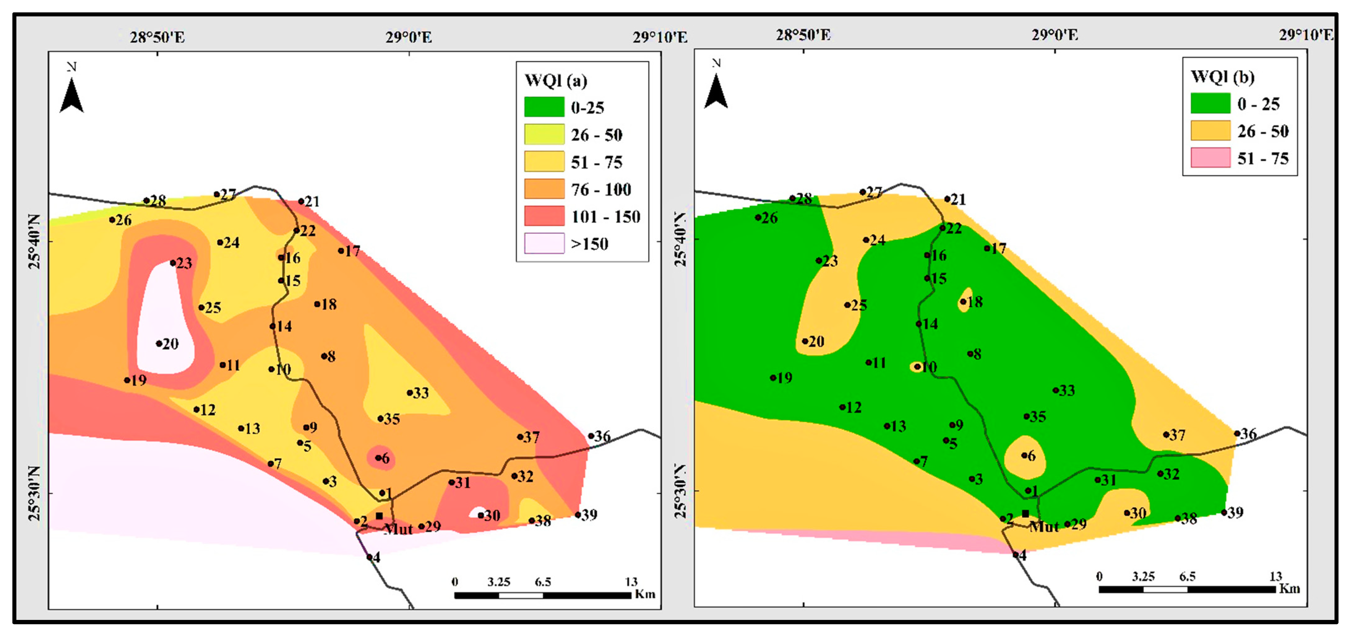
5. Water Quality Index (WQI)

Darwish et al. [13] evaluated the water quality in El-Dakhla for various purposes, considering parameters such as major ions, total salinity, Na%, and Cl⁻. Their findings indicated that the groundwater is rated from excellent to low suitability, while wastewater is deemed unsuitable for any purpose. Meanwhile, Megahed et al. [58,59] employed GIS modeling and hydro-chemical properties to assess the groundwater in El-Dakhla and El-Frafra Oases. Their analysis indicated that the groundwater in El-Dakhla Oasis is suitable for irrigation based on parameters such as total dissolved solids (TDS), the sodium adsorption ratio, and residual sodium carbonate. Furthermore, when evaluating total hardness, Kelly’s ratio, magnesium hazard, pH, and sodium percentage (Na%), most groundwater samples were deemed appropriate for irrigation, even though some samples exceeded the standards for drinking water quality. In El-Frafra Oasis, despite variations in groundwater quality indices (TDS, SO₄⁻², and HCO₃⁻) over time, no significant effects of climatic changes on groundwater quality were observed according to previous studies. The WQI gives a complete summary evaluation of the water quality level of water samples [60,61].

The WQI is a tool that defines water quality. It is necessary to distribute information about water quality in a simple format [23,62,63,64]. Many authors used this method; it was first used by [35] and later applied by [12,25,42,64,65,66,67,68]. In our study, we used the weighted arithmetic water quality index (WA-WQI) [23,64,69]. The relative weight (W_i) is computed by the following equation:

$${\mathrm{W}}_{\mathrm{i}}={\displaystyle \frac{{\mathrm{W}}_{\mathrm{i}}}{{\sum }_{\mathrm{i}=1}^{\mathrm{n}}{\mathrm{W}}_{\mathrm{i}}}}$$

where W_i is the relative weight of the i^th parameter (dimensionless), while n is the number of parameters and w_i is the weight of each parameter. Then the quality rating scale (q_i) is determined for each parameter as follows:

$${\mathrm{q}}_{\mathrm{i}}={\displaystyle \frac{{\mathrm{C}}_{\mathrm{i}}}{{\mathrm{S}}_{\mathrm{i}}}}\times 100$$

where q_i is the quality rating, C_i is the concentration of each chemical parameter in each water sample in (mg/L), except for pH and EC, and S_i is the corresponding value. Then the sub-index (SI_i) is calculated for each parameter (dimensionless) and WQI as follows:

$${\mathrm{SI}}_{\mathrm{i}} = {\mathrm{W}}_{\mathrm{i}} \times {\mathrm{q}}_{\mathrm{i}}$$

Then WQI is calculated as follows:

$$\mathrm{W}\mathrm{Q}\mathrm{I}=\sum _{\mathrm{i}=1}^{\mathrm{n}}{\mathrm{SI}}_{\mathrm{i}}$$

where q_i is the quantity rating based on the concentration of the i^th parameter, n is the number of parameters, and SI_i is the sub-index of the i^th parameter. The WQI serves as a valuable instrument for conveying information about water quality, offering a straightforward, consistent, and demonstrable unit of measurement that proves beneficial for decision-makers and concerned citizens [70]. The WQI is based on many factors used to calculate total water quality [24].

The WQI serves as a measure to evaluate the suitability of groundwater for drinking purposes. In this regard, careful consideration was paid to adhere to the prescribed criteria outlined by the World Health Organization (WHO [52]), and the standards set by the Egypt Decree. In this study, the WQI values were computed by taking into account various parameters. Physical parameters such as pH, total dissolved solids (TDS), and electrical conductivity (EC), as well as major cations (Ca²⁺, K⁺, Mg²⁺, and Na⁺), major anions (Cl⁻, HCO₃⁻, and SO₄²⁻), and certain heavy metals (Fe²⁺ and Mn²⁺) in groundwater were considered. Additionally, other heavy metals including Cr⁺³, Cu⁺², Pb⁺², Ni⁺², and Zn⁺² in wastewater were factored in. Each parameter was assigned a weight (wi) based on its impact on water quality. Parameters significantly influencing water quality, like EC, TDS, Cu⁺², and Cr⁺³, were given a maximum weight of 5, while those with less pronounced effects, such as Ca^2+, Mg²⁺, pH, and HCO₃⁻, were assigned a weight of 2. Parameters like Na⁺, Cl-, Fe²⁺, Mn²⁺, and others received weights ranging from 2 to 4, reflecting their respective influences on the overall water quality, as detailed in

Table 6. WQI parameters used in the study area.

Parameter	Unit	WHO [52]	Weight (Wi)	(Wi)
pH	---	8.5	3	0.107142857
TDS	mg/L	500	5	0.178571429
Ca+2		75	2	0.071428571
Mg+2		30	2	0.071428571
Na+		50	2	0.071428571
Cl−		250	3	0.107142857
SO4−2		200	4	0.142857143
HCO3−		200	3	0.107142857
K+		20	2	0.071428571
Fe2+		0.3	1	0.035714286
Mn2+		0.1	1	0.035714286

. The relative weight (W_i) was calculated according to Gabr et al. [12]. Table 6 summarizes the relative weight (W_i) of groundwater physicochemical parameters for the studied thirty-nine groundwater wells in the study area.

In the study region, the obtained water quality index values (

Table 7. WQI values of the groundwater in the study area.

Well No.	WQI		Well No.	WQI
	Parameters with (Fe2+ and Mn2+)	Parameters without (Fe2+ and Mn2+)		Parameters with (Fe2+ and Mn2+)	Parameters without (Fe2+ and Mn2+)
1	70.5	22.8	21	123	27.5
2	62.8	19.6	22	69.8	23.8
3	60.8	19.4	23	156	24.3
4	297	55.5	24	57.1	25.6
5	61.3	14.7	25	65.3	26.8
6	115	29.4	26	53.1	16.2
7	73.5	18.9	27	52.2	37.5
8	86	18.7	28	43	17.5
9	87	16.9	29	85.9	16.8
10	51.4	25.8	30	168	35.3
11	85.9	22	31	100.8	20.1
12	55.4	17.2	32	88.9	18.8
13	62.5	14.7	33	66.7	16.7
14	91.3	17.6	34	90.2	29.2
15	57.4	9.2	35	69.8	20.6
16	79.7	21.7	36	157	27.8
17	76.8	22.4	37	82.4	28.5
18	84.2	26.5	38	43.3	12
19	90.6	16.2	39	105	23.3
20	278	28

) were categorized as 0–25, 25–50, 51–75, 76–100, and >150, representing excellent, good, poor, very poor, unsuitable, and unfit water quality, respectively.

The values of WQI with iron and manganese concentrations for the groundwater samples in the study area (

Table 8. Water quality index (WQI) ranges for possible usage according to Gabr et al. [12].

WQI Values with (Fe2+ and Mn2+)	Water Quality	Possible Usages	No. of Samples and Percentage
0–25	Excellent	Drinking, irrigation, and industrial	--------
26–50	Good	Domestic, irrigation, and industrial	2 (5%)
51–75	Poor	Irrigation and industrial	15 (38.5%)
76–100	Very poor	Irrigation	12 (30.8%)
101–150	Unsuitable	Restricted use for irrigation	4 (10.3%)
> 150	Unfit for drinking	Proper treatment is required before any use	6 (15.4%)
WQI values Without (Fe2+ and Mn2+)	Water Quality	Possible usages	No. of samples
0–25	Excellent	Drinking, irrigation, and industrial	26 (66.6%)
26–50	Good	Domestic, irrigation, and industrial	12 (30.8%)
51–75	Poor	Irrigation and industrial	1 (2.6%)
76–100	Very poor	Irrigation	-------
101–150	Unsuitable	Restricted use for Irrigation	--------
>150	Unfit for drinking	Proper treatment is required before any use	---------

) and the spatial distribution map of WQI with iron and manganese (Figure 15a) show, for two samples (5%), the WQI values are between 26 and 50, and are acceptable for domestic, irrigation, and industrial uses (good). Fifteen samples (38.5%) were impure, with WQI 51–75, and are acceptable for irrigation and industrial uses (poor), and twelve of the samples (30.8%), with WQI 76–100, are acceptable for irrigation (very poor). A WQI between 101 and 150 was found in four of the samples (10.3%), which restricted their use for irrigation (unsuitable), and a WQI of more than 150 was found in six of the samples (15.4%), for which proper treatment is required before any use (unfit for drinking). The values of WQI without iron and manganese parameters in the groundwater samples in the study area (Table 8), and the spatial distribution map of WQI without iron and manganese parameters (Figure 15b), refer to twenty-six samples (66.6%), for which the WQI values are between 0.0 and 25 and are acceptable for drinking, irrigation, and industrial uses (excellent), and represent most of the study area. Twelve samples (30.8%) were impure, with WQI 26–50, and are acceptable for domestic, irrigation, and industrial uses (good), and one sample (2.6%), with WQI 51–75, is acceptable for irrigation and industrial uses (poor). The values of the WQI in the wastewater samples in the study area are more than 150 (

Table 9. WQI values of the wastewater in the study area.

Wastewater	WQI Values	WQI Values	Possible Usages	No. of Samples
Mut Lake (A)	10,440	>150	Treatment is required before any use	7 (100%)
Mut canal (B)	1300
El-Rashda Lake (C)	4686
El-Rashda canal (D)	511
El-Qalamun Lake (E)	1624
Al-Masarah canal (F)	936
Ismant wastewater canal (G)	932

), so this water needs proper treatment before any use.

6. Conclusions

This study aims to examine the hydro-chemical features of water within the study area, which is encompassed by sedimentary rocks ranging from the Late Cretaceous to the Quaternary periods. The focal point of the investigation is the Taref formation, which is identified as the principal water-bearing stratum in this study, characterized by both good water quality and shallow depths.

The mean TDS in the groundwater is 165 mg/L (freshwater), and that in the wastewater is 30,080 mg/L (brackish to briny water). The mean total hardness of the groundwater is 73.6 mg/L (soft to moderately hard class), while the mean TH of the wastewater is 4676 mg/L (very hard class). The concentrations of Ca⁺², Mg⁺², Na⁺, K⁺, HCO₃⁻, SO₄⁻² and Cl⁻ in the groundwater samples in the study area were below the acceptable limits of WHO, 2011, while those in the wastewater lakes and canals samples were above the acceptable limit of WHO.

The groundwater geochemical evolution in the area is influenced by the dissolution of aquifer materials, as illustrated by Piper’s, Schoeller’s, and Stiff’s diagrams. The groundwater samples show various water types, including sodium–chloride, sodium–bicarbonate, sodium–sulphate, calcium–chloride, calcium–sulphate, and calcium–bicarbonate, while wastewater samples are primarily sodium–chloride. The wastewater chemistry is affected by evaporation, while the groundwater chemistry is controlled by the dissolution of evaporitic minerals.

The water quality index (WQI) indicates that, without considering iron and manganese, 66.6% of groundwater samples are excellent, 30.8% are good, and 2.6% are poor for various uses. When including these parameters, only 5% are good, 38.5% are poor, 30.8% are very poor, 10.3% are unsuitable, and 15.4% are unfit for use. All wastewater samples have WQI values exceeding 150, indicating they require treatment before use.

The current work can be used to understand the hydrochemistry and quality of the groundwater in a compressed area in terms of surface water scarcity, as well as help preserve the groundwater resource and its optimal use for all purposes.

References

1. Khan, H.H.; Khan, A.; Ahmed, S.; Perrin, J. GIS-based impact assessment of land-use changes on groundwater quality: Study from a rapidly urbanizing region of South India. Environ. Earth Sci. 2011, 63, 1289–1302. [Google Scholar] [CrossRef]
2. Siraj, G.; Khan, H.H.; Khan, A. Dynamics of surface water and groundwater quality using water quality indices and GIS in river Tamsa (Tons), Jalalpur, India. HydroResearch 2023, 6, 89–107. [Google Scholar] [CrossRef]
3. Adimalla, N.; Wu, J. Groundwater quality and associated health risks in a semi-arid region of south India: Implication to sustainable groundwater management. Hum. Ecol. Risk Assess. Int. J. 2019, 25, 191–216. [Google Scholar] [CrossRef]
4. Kammoun, S.; Trabelsi, R.; Re, V.; Zouari, K.; Henchiri, J. Groundwater quality assessment in semi-arid regions using integrated approaches: The case of Grombalia aquifer (NE Tunisia). Environ. Monit. Assess. 2018, 190, 1–22. [Google Scholar] [CrossRef] [PubMed]
5. Ostad-Ali-Askari, K.; Shayannejad, M.; Eslamian, S.; Zamani, F.; Shojaei, N.; Navabpour, B.; Majidifar, Z.; Sadri, A.; Ghasemi-Siani, Z.; Nourozi, H. Deficit irrigation: Optimization models. In Handbook of Drought and Water Scarcity; CRC Press: Boca Raton, FL, USA, 2017; pp. 375–391. [Google Scholar]
6. Talebmorad, H.; Ostad-Ali-Askari, K. Hydro geo-sphere integrated hydrologic model in modeling of wide basins. Sustain. Water Resour. Manag. 2022, 8, 118. [Google Scholar] [CrossRef]
7. Bodrud-Doza, M.; Bhuiyan, M.A.H.; Islam, S.D.-U.; Rahman, M.S.; Haque, M.M.; Fatema, K.J.; Ahmed, N.; Rakib, M.; Rahman, M.A. Hydrogeochemical investigation of groundwater in Dhaka City of Bangladesh using GIS and multivariate statistical techniques. Groundw. Sustain. Dev. 2019, 8, 226–244. [Google Scholar] [CrossRef]
8. Mallick, J.; Singh, C.K.; AlMesfer, M.K.; Kumar, A.; Khan, R.A.; Islam, S.; Rahman, A. Hydro-geochemical assessment of groundwater quality in Aseer Region, Saudi Arabia. Water 2018, 10, 1847. [Google Scholar] [CrossRef]
9. Egbueri, J.C.; Unigwe, C.O.; Omeka, M.E.; Ayejoto, D.A. Urban groundwater quality assessment using pollution indicators and multivariate statistical tools: A case study in southeast Nigeria. Int. J. Environ. Anal. Chem. 2023, 103, 3324–3350. [Google Scholar] [CrossRef]
10. Abrahão, R.; Causapé, J.; García-Garizábal, I.; Merchán, D. Implementing irrigation: Water balances and irrigation quality in the Lerma basin (Spain). Agric. Water Manag. 2011, 102, 97–104. [Google Scholar] [CrossRef]
11. Wang, Z.; Wang, L.-J.; Shen, J.-M.; Nie, Z.-L.; Meng, L.-Q.; Cao, L.; Wei, S.-B.; Zeng, X.-F. Groundwater characteristics and climate and ecological evolution in the Badain Jaran Desert in the southwest Mongolian Plateau. China Geol. 2021, 4, 421–432. [Google Scholar] [CrossRef]
12. Gabr, M.E.; Soussa, H.; Fattouh, E. Groundwater quality evaluation for drinking and irrigation uses in Dayrout city Upper Egypt. Ain Shams Eng. J. 2021, 12, 327–340. [Google Scholar] [CrossRef]
13. Darwish, M.H.; Sayed, A.G.; Hassan, S.H. Assessment of Water for Different Uses at Some Localities of the Dakhla Oasis, Western Desert, Egypt. Water Air Soil Pollut. 2023, 234, 516. [Google Scholar] [CrossRef]
14. Massoud, M.A. Assessment of water quality along a recreational section of the Damour River in Lebanon using the water quality index. Environ. Monit. Assess. 2012, 184, 4151–4160. [Google Scholar] [CrossRef] [PubMed]
15. Rosemond, S.D.; Duro, D.C.; Dubé, M. Comparative analysis of regional water quality in Canada using the Water Quality Index. Environ. Monit. Assess. 2009, 156, 223–240. [Google Scholar] [CrossRef]
16. Kannel, P.R.; Lee, S.; Lee, Y.-S.; Kanel, S.R.; Khan, S.P. Application of water quality indices and dissolved oxygen as indicators for river water classification and urban impact assessment. Environ. Monit. Assess. 2007, 132, 93–110. [Google Scholar] [CrossRef]
17. Boyacioglu, H.; Boyacioglu, H. Surface water quality assessment by environmetric methods. Environ. Monit. Assess. 2007, 131, 371–376. [Google Scholar] [CrossRef] [PubMed]
18. Debels, P.; Figueroa, R.; Urrutia, R.; Barra, R.; Niell, X. Evaluation of water quality in the Chillán River (Central Chile) using physicochemical parameters and a modified water quality index. Environ. Monit. Assess. 2005, 110, 301–322. [Google Scholar] [CrossRef]
19. Cox, C.R.; World Health Organization. Operation and Control of Water Treatment Processes; World Health Organization: Geneva, Switzerland, 1964.
20. Horton, R.K. An index number system for rating water quality. J. Water Pollut. Control Fed. 1965, 37, 300–306. [Google Scholar]
21. Drever, J.I. The Geochemistry of Natural Waters: Surface and Groundwater Environments; Prentice Hall: Hoboken, NJ, USA, 1997. [Google Scholar]
22. Akter, T.; Jhohura, F.T.; Akter, F.; Chowdhury, T.R.; Mistry, S.K.; Dey, D.; Barua, M.K.; Islam, M.A.; Rahman, M. Water Quality Index for measuring drinking water quality in rural Bangladesh: A cross-sectional study. J. Health Popul. Nutr. 2016, 35, 4. [Google Scholar] [CrossRef] [PubMed]
23. Asadi, E.; Isazadeh, M.; Samadianfard, S.; Ramli, M.F.; Mosavi, A.; Nabipour, N.; Shamshirband, S.; Hajnal, E.; Chau, K.-W. Groundwater quality assessment for sustainable drinking and irrigation. Sustainability 2019, 12, 177. [Google Scholar] [CrossRef]
24. Chen, J.; Huang, Q.; Lin, Y.; Fang, Y.; Qian, H.; Liu, R.; Ma, H. Hydrogeochemical characteristics and quality assessment of groundwater in an irrigated region, Northwest China. Water 2019, 11, 96. [Google Scholar] [CrossRef]
25. Cash, K.; Wright, R. Canadian Water Quality Guidelines for the Protection of Aquatic Life; CCME: Ottawa, ON, Canada, 2001. [Google Scholar]
26. Ranganathan, M.; Karuppannan, S.; Murugasen, B.; Brhane, G.K.; Panneerselvam, B. Assessment of groundwater prospective zone in Adigrat Town and its surrounding area using geospatial technology. In Climate Change Impact on Groundwater Resources: Human Health Risk Assessment in Arid and Semi-Arid Regions; Springer: Berlin/Heidelberg, Germany, 2022; pp. 387–405. [Google Scholar]
27. Darwish, M.H.; Galal, W.F. Spatiotemporal effects of wastewater ponds from a geoenvironmental perspective in the Kharga region, Egypt. Prog. Phys. Geogr. Earth Environ. 2020, 44, 376–397. [Google Scholar] [CrossRef]
28. Darwish, M.H.; Megahed, H.A.; Farrag, A.E.-H.A.; Sayed, A.G. Geo-Environmental Changes and Their Impact on the Development of the Limestone Plateau, West of Assiut, Egypt. J. Indian Soc. Remote Sens. 2020, 48, 1705–1727. [Google Scholar] [CrossRef]
29. Galal, W.F.; Darwish, M.H. Geoenvironmental assessment of the mut wastewater ponds in the Dakhla Oasis, Egypt. Geocarto Int. 2022, 37, 3293–3311. [Google Scholar] [CrossRef]
30. Brookes, I.A. Geomorphology and Quaternary geology of the Dakhla Oasis region, Egypt. Quat. Sci. Rev. 1993, 12, 529–552. [Google Scholar] [CrossRef]
31. Egyptian Meteorological Authority. Climatic Atlas of Egypt; Arab Republic of Egypt, Ministry of Transport: Cairo, Egypt, 1996.
32. Ghoubachi, S. Hydrogeological Characteristics of the Nubia Sandstone Aquifer System in Dakhla Depression, Western Desert Egypt. Master’s Thesis, Faculty of Science, Ain Shams University, Cairo, Egypt, 2001. [Google Scholar]
33. Hermina, M. The surroundings of Kharga, Dakhla and Farafra oases. In The Geology of Egypt; Routledge: Oxfordshire, UK, 2017; pp. 259–292. [Google Scholar]
34. Awad, G.H. Zonal stratigraphy of Kharga Oasis. Ann. Geol. Surv. Egypt 1966, 34, 1–77. [Google Scholar]
35. Issawi, B. Review of Upper Cretaceous-Lower Tertiary stratigraphy in central and southern Egypt. AAPG Bull. 1972, 56, 1448–1463. [Google Scholar]
36. Pachur, H.-J. Paläo-Environment und Drainagesysteme der Ostsahara im Spätpleistozän und Holozän. In Nordost-Afrika Strukturen und Ressourcen. Deutsche Forschungemeinschaft; Wiley-VCH Verlag: Weinheim, Germany, 1999. [Google Scholar]
37. Said, R. The Geology of Egypt; Routledge: Oxfordshire, UK, 2017. [Google Scholar]
38. Thorweihe, U.; Heinl, M. Grundwasserressourcen im Nubischen Aquifersystem. In Nordost-Afrika Strukturen und Ressourcen. Deutsche Forschungemeinschaft; Wiley-VCH Verlag: Weinheim, Germany, 1999. [Google Scholar]
39. Van Ginkel, S.W.; Hassan, S.H.A.; Oh, S.E. Detecting endocrine disrupting compounds in water using sulfur-oxidizing bacteria. Chemosphere 2010, 81, 294–297. [Google Scholar] [CrossRef] [PubMed]
40. Rice, E.W.; Bridgewater, L.; American Public Health Association (Eds.) Standard Methods for the Examination of Water and Wastewater; American Public Health Association: Washington, DC, USA, 2012; Volume 10. [Google Scholar]
41. Raghunath, H.M. Ground Water: Hydrogeology, Ground Water Survey and Pumping Tests, Rural Water Supply and Irrigation Systems; New Age International: New Delhi, India, 1987. [Google Scholar]
42. Appelo, C.; Postma, D. Geochemistry, Groundwater and Pollution, 2nd ed.; Balkema: Leiden, The Netherlands, 2005. [Google Scholar]
43. Dahab, K. Review on the hydrostratigraphic section in Egypt with special emphasis on their recharging sources. Bull. Geol. Surv. Cairo Egypt 1998, 45, 61–89. [Google Scholar]
44. Idris, H.; Nour, S. Present groundwater status in Egypt and the environmental impacts. Environ. Geol. Water Sci. 1990, 16, 171–177. [Google Scholar] [CrossRef]
45. Davis, S.N.; DeWiest, R.J. Hydrogeology; John Wiley and Sons: New York, NY, USA, 1966. [Google Scholar]
46. Hem, J.D. Study and Interpretation of the Chemical Characteristics of Natural Water, 2nd ed.; US Government Printing Office: Washington, DC, USA, 1970.
47. Hem, J.D. Study and Interpretation of the Chemical Characteristics of Natural Water, 3rd ed.; Department of the Interior, US Geological Survey: Reston, VA, USA, 1985.
48. Saber, M.; Mokhtar, M.; Bakheit, A.; Elfeky, A.M.; Gameh, M.; Mostafa, A.; Sefelnasr, A.; Kantoush, S.A.; Sumi, T.; Hori, T.; et al. An integrated assessment approach for fossil groundwater quality and crop water requirements in the El-Kharga Oasis, Western Desert, Egypt. J. Hydrol. Reg. Stud. 2022, 40, 101016. [Google Scholar] [CrossRef]
49. Porter, D.O.; Marek, T. Irrigation management with saline water. In Proceedings of the 2006 Central Plains Irrigation Conference, Colby, KS, USA, 21–22 February 2006; Colorado State University Libraries: Fort Collins, CO, USA, 2006. [Google Scholar]
50. Rabeiy, R.E. Assessment and modeling of groundwater quality using WQI and GIS in Upper Egypt area. Environ. Sci. Pollut. Res. 2018, 25, 30808–30817. [Google Scholar] [CrossRef] [PubMed]
51. World Health Organization. Guidelines for Drinking-Water Quality; World Health Organization: Geneva, Switzerland, 2011; Volume 216, pp. 303–304.
52. Correns, C.W. The geochemistry of the halogens. Phys. Chem. Earth 1956, 1, 181–233. [Google Scholar] [CrossRef]
53. Fipps, G. Irrigation Water Quality Standards and Salinity Management Strategies; Texas FARMER Collection: Waco, TX, USA, 2003.
54. Am, P. A graphic procedure in the geochemical interpretation of water analysis. Trans.-Am. Geophys. Union 1944, 25, 914–923. [Google Scholar]
55. Scholler, H. Geochemie des eaux souterraines. Rev. De I’institut Fr. Du Pet. 1962, 10, 230–244. [Google Scholar]
56. Kumar, P. Interpretation of groundwater chemistry using piper and Chadha’s diagrams: A comparative study from Perambalur Taluk. Elixir Geosci. 2013, 54, 12208–12211. [Google Scholar]
57. Stiff, H.A., Jr. The interpretation of chemical water analysis by means of patterns. J. Pet. Technol. 1951, 3, 15. [Google Scholar] [CrossRef]
58. Megahed, H.A.; GabAllah, H.M.; AbdelRahman, M.A.; D’Antonio, P.; Scopa, A.; Darwish, M.H. Geomatics-Based Modeling and Hydrochemical Analysis for Groundwater Quality Mapping in the Egyptian Western Desert: A Case Study of El-Dakhla Oasis. Water 2022, 14, 4018. [Google Scholar] [CrossRef]
59. Megahed, H.A.; GabAllah, H.M.; Ramadan, R.H.; AbdelRahman, M.A.; D’Antonio, P.; Scopa, A.; Darwish, M.H. Groundwater Quality Assessment Using Multi-Criteria GIS Modeling in Drylands: A Case Study at El-Farafra Oasis, Egyptian Western Desert. Water 2023, 15, 1376. [Google Scholar] [CrossRef]
60. Igwe, O.; Omeka, M. Hydrogeochemical and pollution assessment of water resources within a mining area, SE Nigeria, using an integrated approach. Int. J. Energy Water Resour. 2022, 6, 161–182. [Google Scholar] [CrossRef]
61. Xiao, Y.; Liu, K.; Yan, H.; Zhou, B.; Huang, X.; Hao, Q.; Zhang, Y.; Zhang, Y.; Liao, X.; Yin, S. Hydrogeochemical constraints on groundwater resource sustainable development in the arid Golmud alluvial fan plain on Tibetan plateau. Environ. Earth Sci. 2021, 80, 1–17. [Google Scholar] [CrossRef]
62. Gao, Y.; Qian, H.; Ren, W.; Wang, H.; Liu, F.; Yang, F. Hydrogeochemical characterization and quality assessment of groundwater based on integrated-weight water quality index in a concentrated urban area. J. Clean. Prod. 2020, 260, 121006. [Google Scholar] [CrossRef]
63. Tirkey, P.; Bhattacharya, T.; Chakraborty, S.; Baraik, S. Assessment of groundwater quality and associated health risks: A case study of Ranchi city, Jharkhand, India. Groundw. Sustain. Dev. 2017, 5, 85–100. [Google Scholar] [CrossRef]
64. Batabyal, A.K.; Chakraborty, S. Hydrogeochemistry and water quality index in the assessment of groundwater quality for drinking uses. Water Environ. Res. 2015, 87, 607–617. [Google Scholar] [CrossRef]
65. Ramakrishnaiah, C.; Sadashivaiah, C.; Ranganna, G. Assessment of water quality index for the groundwater in Tumkur Taluk, Karnataka State, India. J. Chem. 2009, 6, 523–530. [Google Scholar]
66. Sahoo, S.; Khaoash, S. Impact assessment of coal mining on groundwater chemistry and its quality from Brajrajnagar coal mining area using indexing models. J. Geochem. Explor. 2020, 215, 106559. [Google Scholar] [CrossRef]
67. Samal, P.; Mohanty, A.K.; Khaoash, S.; Mishra, P. Hydrogeochemical evaluation, groundwater quality appraisal, and potential health risk assessment in a coal mining region of Eastern India. Water Air Soil Pollut. 2022, 233, 324. [Google Scholar] [CrossRef]
68. Silva, M.; Gonçalves, A.; Lopes, W.; Lima, M.; Costa, C.; Paris, M.; Firmino, P.; De Paula Filho, F. Assessment of groundwater quality in a Brazilian semiarid basin using an integration of GIS, water quality index and multivariate statistical techniques. J. Hydrol. 2021, 598, 126346. [Google Scholar] [CrossRef]
69. Şener, Ş.; Şener, E.; Davraz, A. Evaluation of water quality using water quality index (WQI) method and GIS in Aksu River (SW-Turkey). Sci. Total Environ. 2017, 584, 131–144. [Google Scholar] [CrossRef]
70. Tiwari, A.K.; Singh, A.K.; Mahato, M.K. Assessment of groundwater quality of Pratapgarh district in India for suitability of drinking purpose using water quality index (WQI) and GIS technique. Sustain. Water Resour. Manag. 2018, 4, 601–616. [Google Scholar] [CrossRef]
Figure 1. Location of the study area and water samples. Groundwater samples are presented by solid red circles and numbered 1–39. The wastewater samples are marked by letters A–G.
Hydrology 11 00160 g001
Figure 2. The geological map of the study area (modified after [13]).
Hydrology 11 00160 g002
Figure 3. Histogram showing the chemical analysis of water samples.
Hydrology 11 00160 g003
Figure 4. Histogram showing the chemical analysis of the wastewater samples.
Hydrology 11 00160 g004
Figure 5. The spatial distribution of the pH, TH, SO4−2, Cl, Fe+2, and Mn+2 in the water samples.
Hydrology 11 00160 g005
Figure 6. The spatial distribution of the TDS, pH, Ca+2, Mg+2, Na+, and K+ in the wastewater.
Hydrology 11 00160 g006
Figure 7. The spatial distribution of the TDS, Ca+2, Mg+2, Na+, K+, and HCO3 in the groundwater samples.
Hydrology 11 00160 g007
Figure 8. The spatial distribution of the TH, HCO3, Cl, and SO4−2 in the wastewater.
Hydrology 11 00160 g008
Figure 9. The spatial distribution of the trace elements in the wastewater in the study area.
Hydrology 11 00160 g009
Figure 10. Piper trilinear diagram for classification of the water samples.
Hydrology 11 00160 g010
Figure 11. Semi-logarithmic diagram for the groundwater samples.
Hydrology 11 00160 g011
Figure 12. Semi-logarithmic diagram, Schoeller diagram [57], for the wastewater samples.
Hydrology 11 00160 g012
Figure 13. Stiff diagram of major-ion chemistry of the water samples.
Hydrology 11 00160 g013
Figure 14. Stiff diagram of major-ion chemistry of the wastewater samples.
Hydrology 11 00160 g014
Figure 15. The spatial distribution maps of the WQI values in the study area: (a) WQI distribution with Fe2+ and Mn2+concentrations; (b) WQI distribution without Fe2+ and Mn2+concentrations.
Hydrology 11 00160 g015