Abstract
On the southeastern coast of Brazil, the bays of Ilha Grande and Sepetiba are linked by the Ilha Grande Channel, where remarkably strong currents have been consistently observed. Tidal forces cannot explain the strength of these currents. Previous researchers have focused on investigating factors like baroclinic effects due to salinity differences or seiches between two basins without a conclusive answer. This study aims to elucidate the role of remote meteorological effects within this complex hydrodynamic system. A numerical approach with a coastal model nested within an ocean model was employed, enabling an in-depth examination of the intricate interplay between meteorological and tidal forcings. The study revealed a significant finding: the lag in signal propagation plays a pivotal role in determining how these signals impact the dynamics of the bays. The astronomical signal exhibits a minimal lag along the coast (1 min) and leads to water level differences between the sea and the coastline, resulting in the generation of tidal currents at the bay entrances. On the other hand, the remote meteorological signal, with a stronger signal lag along the coast (4.92 h), leads to the creation of a water level difference between the bay entrances, inducing significant fluxes along the narrow Ilha Grande Channel.
1. Introduction
A coastal region represents a dynamic interface where terrestrial, marine, and atmospheric systems intersect and where the actions of humans not only impact the coastal area but are also influenced by the integrated behavior of these three interconnected domains. This unique setting is vulnerable to various hazards, including erosion, subsidence, tsunamis, and flooding, all of which can be exacerbated by rising sea levels and river floods [1]. Moreover, when astronomical and meteorological factors combine, they can give rise to extreme sea level events, which pose a substantial threat to coastal communities and ecosystems, as well as the destruction of critical ports and coastal structures [2]. As noted by Mestres et al. [3], port authorities have increasingly focused on this phenomenon due to its potential to impede the safe maneuvering, approach, and entry of ships into ports, thus posing a risk of accidents. This combination of factors has been a significant contributor to disasters, as reported by the World Meteorological Organization [4], accounting for 44% of recorded disasters and 31% of economic losses between 1970 and 2019. It underscores the urgent need for a comprehensive understanding and management of coastal dynamics to mitigate these risks effectively.
The sea level temporal variation (η(t)) can be written, according to Pugh [5], as
Slow variations in time, η0(t): This component accounts for gradual changes in sea levels over time and can often be approximated by averaging for shorter time scales. It encompasses interannual and long-term variability, which are linked to eustatic (global sea level changes) and isostatic (crustal adjustments) processes.
The astronomical component, ηA(t): The astronomical component of sea level variation primarily arises from tidal-generating forces, as indicated by research by Bowden [6] and Open University [7]. Tides, in general, constitute the predominant driver of sea level fluctuations along coastlines, as emphasized by Pugh [5].
The meteorological component, ηM(t): The meteorological component represents the difference between the observed sea level and the astronomical signal, as described by Marone and Camargo [8] and Pugh [5]. This component captures the influence of meteorological factors on sea levels. Importantly, Marone and Camargo [8] note that only about 10% of this residual signal is typically attributed to changes in atmospheric pressure, while the majority is associated with wind-induced friction on the sea surface. This wind-induced friction can generate oscillations in sea level, which can originate either locally or remotely.
These oscillations may occur as coastal trapped waves (CTW), which are categorized into two main types: Supra-inertial waves (edge waves): these CTWs occur at frequencies higher than the Earth’s inertial frequency. They can be excited by various meteorological forcings, including changes in atmospheric pressure (the inverted barometer effect), wind wave radiation in shallow water, and wave refraction and diffraction effects. These forcings typically have a localized impact on water levels [5,8]. Subinertial waves: These CTWs occur at frequencies lower than the Earth’s inertial frequency and are primarily associated with remote origins [5]. The Ekman transport associated with wind parallel to the coast can generate these subinertial waves. This results in an oscillatory motion that remains trapped along the coast through geostrophic balance [9,10] with a cyclonic direction of propagation. These waves carry energy from the wind-affected area to other coastal regions [11]. These subinertial oscillations are influenced by the Earth’s rotation [12], with the Coriolis force acting as a restoring mechanism.
In summary, sea level variation is a multifaceted phenomenon shaped by slow temporal changes, astronomical forces (primarily tides), and meteorological factors (especially wind-induced effects), where coastal trapped waves play a crucial role in understanding the complex dynamics of coastal sea level fluctuations.
The term “storm surges,” as defined by Idier et al. [13], refers to long waves that arise from changes in atmospheric pressure and the stress of wind on the sea surface. These waves propagate along coastlines as shallow water waves and are subject to various influences, including bottom friction, the Earth’s rotation (Coriolis force), and local amplifications due to resonant effects.
Wang and Elliott [14] conducted a study on estuarine circulation at Chesapeake Bay and observed that most non-tidal fluctuations occur on seasonal and storm time scales. They also noted that during certain periods, remote wind forcing dominates over local effects, underscoring the importance of considering both factors in estuarine circulation modeling. While local wind patterns play a prominent role in the upper estuary, affecting the slope between high and low estuary water levels, remote forcings impact the lower estuary, propagating as long waves into bays with minimal dissipation or amplification [15,16].
Melo Filho [17] discusses two approaches for simulating the remote wind effect. The first approach involves statistical methods, such as cross-correlation, linear regression models (as used by Truccolo et al. [18]), or neural network models (as employed by Oliveira et al. [19]). These statistical models rely on extensive databases to establish relationships between wind and water level changes. The second approach involves coupling coastal and oceanic numerical models using the nesting technique. In this way, coastal models simulate local hydrodynamics, taking the effects of large and mesoscale oceanic and atmospheric circulation into account. In numerical coastal studies, it is common for ocean models to provide boundary conditions for coastal models through grid nesting, as demonstrated by various studies [16,20,21,22]. This approach allows for a more comprehensive representation of the complex interactions between remote and local factors in coastal areas and their impact on estuarine circulation.
The southern and southeastern coasts of Brazil fall under the influence of low-pressure frontal systems that interact with the western branch of the South Atlantic high-pressure system. The cold fronts linked to these low-pressure systems exhibit a seasonal pattern, being more frequent in Brazil during the austral autumn and winter [2], leading to shifts in wind direction. According to Veleda et al. [23], the combination of wind friction and the abrupt changes in coastline orientation between 22° S and 36° S along the Brazilian coast make this region particularly prone to generating coastal trapped waves (CTWs).
The irregularities in the bathymetry of the continental shelf result in alterations in the characteristics of CTWs, including a decrease in propagation speed and amplitude [11,24]. Freitas et al. [25] suggest that this is evident along the southeastern Brazilian coast, where a decrease in CTW energy and phase speed propagation is observed towards the northern limit (around 22° S, between Tubarão Bight and Abrolhos Bank). This region features abrupt variations in the width and depth of the continental shelf.
Several studies, including Sandstrom [26], Truccolo et al. [18], and Andrade et al. [2], have emphasized the significance of the non-astronomical signal on sea levels caused by CTWs along the south and southeastern Brazilian coast. Meteorological events, particularly wind changes resulting from cold fronts along the southeastern Brazilian coast, can induce water level variations of a magnitude comparable to tidal effects [27]. Andrade et al. [2] conducted a data analysis on the Rio Grande do Sul coast, revealing an average tidal variation of 0.30 m. However, when the tidal signal was excluded, the water level signal reached up to 0.40 m, underscoring the critical importance of studying the non-astronomical signal in this coastal area.
A study by Castro and Lee [28] conducted on the south–southeast Brazilian continental shelf revealed that sea level fluctuations exhibit periods ranging from 9 to 12 days and from 6 to 7 days. These fluctuations were found to be closely correlated with southern winds that occurred before the passage of these oscillations. Additionally, the presence of coastal trapped waves was reported in the same area by França [29]. These waves are responsible for a significant portion of the energy propagated at subinertial frequencies towards the north, potentially leading to variations in current intensity within the subinertial band [30].
The inertial period can be obtained by
where f is the Coriolis parameter, Ω is the angular velocity of the Earth (Ω = 2π/T), and θ is the local latitude. For the latitude of the study area, 23° S, the inertial period is 30.7 h.
Melo Filho [8] conducted a study indicating that the variance of the subinertial signal associated with remote winds (with periods ranging between 3 and 30 days) along the Rio de Janeiro coast represents 66.0% of the total variance. Seasonality (periods ranging between 30 days and 1 year) accounts for 28.2%, while local winds (with periods ranging between 2 h and 3 days) contribute 5.8%. Similar findings were reported by Rodrigues et al. [31], who found that 67.5% of the total signal variance corresponds to the subinertial along-channel currents component, featuring periods ranging from 2 to 30 days. Melo Filho [8] also noted that 50% of the meteorological influence in Rio de Janeiro originates from the area south of Imbituba, while 30% arises from the region between Imbituba and Rio de Janeiro.
The significance of flows related to various forces has been widely acknowledged in studies, including factors such as local wind friction and density [32,33,34]. However, as noted by Kjerfve et al. [35], for the Ilha Grande Channel, wind and ocean dynamics take on a paramount role in local hydrodynamics, accounting for 67% of the annual variation in sea levels. In contrast, atmospheric pressure explains 5% of the annual sea level variation, while steric changes associated with shifts in temperature and salinity within the water column contribute to the remaining 28%.
Fragoso [36] observed an increase in current intensity in the Ilha Grande Channel, reaching up to 0.4 m per second (more than 65%), attributed to meteorological effects. Cavalcante [37] associated currents with meteorological forcing, with intensities reaching around 0.4 m per second in Ilha Grande Bay, approximately 0.05 m per second in Sepetiba Bay, and up to 0.6 m per second in the Ilha Grande Channel.
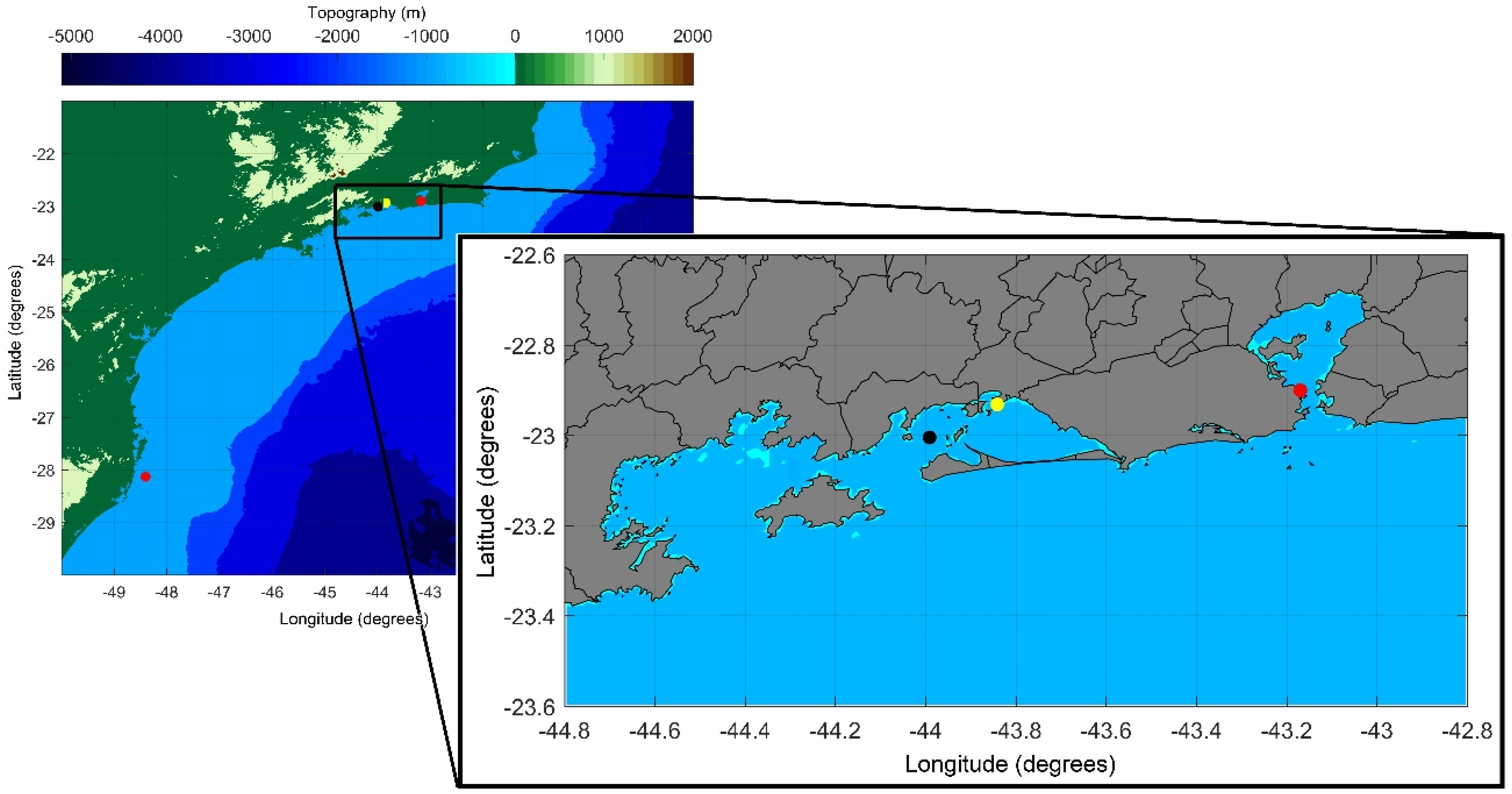
The primary objective of this study is to understand the role of the remote meteorological signal in intensifying currents within the Ilha Grande Channel (Figure 1). To achieve this objective, the research will investigate the patterns of both the remote meteorological signal and tides within Sepetiba and Ilha Grande Bays using a coastal model nested within an ocean model.
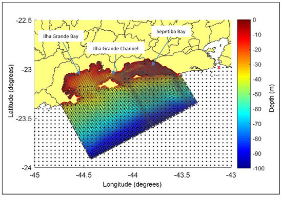
Figure 1.
Location of Ilha Grande and Sepetiba bays on the southeastern coast of Brazil. Thin gray lines represent the grid of the coastal model domain; thick gray lines represent the open boundary. Cyan line indicates the Ilha Grande Channel, and the color palette (in meters) is the bathymetry used (a composition of nautical charts from the Brazilian Navy). Black dots indicate part of the HYCOM 1/24° grid. The red cross in Guanabara Bay’s mouth is the HYCOM point used to compare its results with data.
2. Materials and Methods
2.1. Study Area
The study area encompasses the complex of the Sepetiba and Ilha Grande Bays, situated on the southeastern coast of Brazil (see Figure 1). Sepetiba Bay is characterized by intensive port activity, notably hosting the Port of Itaguaí, which ranks as the second-largest Brazilian port in terms of cargo flow [38]. In contrast, Ilha Grande Bay is primarily utilized for tourism and recreational purposes, as highlighted by Kjerfve et al. [35]. The two bays are interconnected through the Ilha Grande Channel, which also houses an oil terminal among its features.
Sepetiba Bay is characterized by shallower depths and is sheltered from the open sea by the Marambaia sandbar. It has a narrow channel known as the Bacalhau channel that connects it to the open sea on the eastern side. In contrast, Ilha Grande Bay has greater depths and a broader connection to the open sea. These two bays are linked by the Ilha Grande Channel. Ilha Grande Bay receives a comparatively smaller amount of freshwater input from rivers when compared to Sepetiba Bay.
The hydrodynamics of Sepetiba Bay are marked by a robust semidiurnal tidal circulation, which is more pronounced than in Ilha Grande Bay [33,35]. During spring tides, the astronomical tide can reach heights exceeding 1.41 m in Sepetiba Bay and 1.14 m in Ilha Grande Bay, considering the superposition of diurnal and semidiurnal tides [35].
One noteworthy aspect of an astronomical tide is the principal non-linear tidal constituent known as M4. In Ilha Grande Bay, the amplitude of the M4 component ranges from 0.03 to 0.09 m, while in Sepetiba Bay, it ranges from 0.06 to 0.23 m, possibly due to its shallower depths. Additionally, aside from the tidal asymmetry brought about by this constituent, there is a seiche system with a node in the Ilha Grande Channel that appears at nearly quarter-diurnal frequency [35].
As per a numerical study conducted by Harari and Camargo [39], the M2 component has amplitudes reaching approximately 0.25 m in the coastal region from Rio de Janeiro to Cabo Frio. The S2 tidal constituent is around 0.16 m. Both of these constituents exhibit two propagation systems, one from the northeast and one from the southwest, with their convergence point in the Santos region, about 200 km south of the study area. The convergence of these two fronts results in minimal phase differences among the main tidal constituents along the coast [39].
2.2. Hydrodynamic Numerical Modelling
The study employs a one-way nesting method, wherein information is transferred from the ocean model, the Hybrid Coordinate Ocean Model (HYCOM) [40,41], to the more refined model, Delft3D [42]. This approach is widely utilized and allows for information to be passed from a lower-resolution model to a higher-resolution model in a smaller area, combining the benefits of both. The ocean model (HYCOM) is essential for considering remote effects, while the small-scale model (Delft3D) focuses on resolving topography and local features, enabling accurate predictions of sea level and currents, especially in coastal areas [43]. The hydrodynamic module of the Delft3D model [42] was employed for simulating the sea level and currents in the coastal region. Fragoso [36] studied the baroclinic circulation in the study area, concluding that the horizontal pressure gradient from density variability is insufficient to explain the circulation in the area. The author suggested that the channel’s currents intensification can result by a barotropic gradient pressure caused by differences in the sea level in the east–west portions of the bays. Thus, a 2D simulation was chosen to optimize computational efficiency.
The model domain and grid resolution vary, with resolutions ranging from 530 to 2060 m, as indicated in Figure 1. Boundary conditions for the coastal model (elevation and barotropic velocity) were derived from the results of a numerical simulation carried out with the HYCOM developed at the Physical Oceanography Laboratory of COPPE/UFRJ [44,45] within the context of the REMO Project [46], a Brazilian initiative in operational oceanography. These results correspond to a synoptic and assimilative nested simulation with high spatial resolution (1/24°). This simulation considers the eight main diurnal and semidiurnal tidal constituents (M2, S2, N2, K2, O1, P1, K1, Q1) based on the global model TPXO [47].
The bathymetric data used in the study are derived from nautical charts provided by the Diretoria de Hidrografia e Navegação (DHN)/Centro de Hidrografia da Marinha (CHM). Specifically, the nautical charts numbered 162101, 162102, 162301, 163101, 163301, and 231002 were digitized and incorporated into the model. Information on bottom sediment distribution was obtained from previous studies by Ponçano [48] and Mahiques [49] that focused on sediment distribution in the study region. The roughness parameters used in the model were calculated based on the bathymetric and sediment data, following the approach outlined by Nikuradse [50]. These parameters are crucial for accurately representing the frictional effects on water flow.
The open boundary conditions are designed to allow waves to pass through without significant alteration. To minimize the effects of reflection at the boundaries, weakly reflective boundary conditions are utilized, as suggested by Diederen et al. [51]. The boundary conditions assume that there is no flow along the boundary. This simplification is based on the use of Riemann’s invariants for a 1D linearized normal equation at an open boundary. This approach disregards the effects of Coriolis force and bottom stress, focusing on the essential aspects of the boundary conditions [42,52].
Riemann’s invariants are fundamental principles that guide the formulation of open boundary conditions. These invariants suggest that any solution for a subcritical flow is composed of information that is advected in both positive and negative directions [42]. Consequently, two long waves move in opposite directions with a propagation speed described by a specific equation. The direction of wave propagation relative to the adopted mesh’s orientation influences the signal in the equation. The Riemann’s invariants for the 1D equation normal to the open boundary are given by
where U is the normal velocity component; g is the acceleration of gravity; d is the depth; and η is the water level variability. The linearized Riemann’s invariant is given by Equation (3) for a positive direction of propagation relative to the adopted mesh. This condition can only be applied in cases where the variations in the water level are small when compared to the depth [53]. Thus, (3) can be approximated to (4). Therefore, we can impose the boundary conditions on the model in the form of a composition of the sea level and the current component perpendicular to the boundary at each time step.
The reflection of wave signals, as described by Riemann’s invariants, increases significantly as the incidence angle of the wave signal increases. This relationship is established in research by Verboom and Slob [52]. To minimize the effects of wave reflection and ensure accurate boundary conditions, it is crucial to align the orientation of the boundaries appropriately. Specifically, the orientation of the boundaries should either be parallel or perpendicular to the isobars. This alignment helps reduce the impact of wave reflection and ensures that the boundaries allow waves to pass through with minimal alteration.
Four different modeling scenarios were considered: Scenario 1 (S1) involves the full signal (levels and barotropic velocities) from the HYCOM and utilizes Riemann invariants as the open boundary condition. Scenario 2 (S2) isolates the behavior of the astronomical signal, specifically focusing on periods less than 3 days in comparison to the full signal. In scenario 3 (S3), the model examines the flow behavior considering only the astronomical component M2, with a lag time of 1 min between the west and east borders. This lag corresponds to the observed lag for M2. Scenario 4 (S4), similar to Scenario 3, also considers only the astronomical component M2. However, in this case, a lag time of 4.92 h is used, corresponding to the observed lag in the main meteorological component with a period of 4.7 days, as will be discussed in Section 3.3.
These modeling scenarios allow for a comprehensive examination of the role of different components of the signal and the influence of lag times on flow behavior within the study area. A summary of the structures of the adopted modeling scenarios is presented in Figure 2.
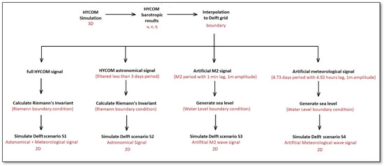
Figure 2.
Flowchart of the information on the structures of the adopted modeling scenarios.
2.3. Data Analysis and Numerical Results Validation
The simulations for scenarios S1 and S2 were conducted for the year 2009. This choice was based on the availability of results from the ocean model, HYCOM, for that specific year. To validate and compare the model results, data from two monitoring stations within Sepetiba Bay were used. These stations provided measurements of sea levels and currents, but for different years than the available HYCOM simulations.
The water level data for Sepetiba Bay were obtained from two sources: Guaíba Island for the period from 6 August 2011 to 26 October 2011 [54] and Port of Itaguaí from 23 November 2011 to 30 April 2012 (MICROARS Consultoria e Projetos LTDA, Rio de Janeiro, Brazil) (Figure 3). Time series data comprise a combination of linear components, periodic or quasi-periodic components, and high-frequency signals. To isolate the meteorological signal from the high-frequency components, a spectral filter with a high-pass filter using a Discrete Fourier Transform was applied. This process was performed in MATLAB R2019a, following the method described by Cerqueira et al. [55]. The high-pass filter effectively removes signals with periods smaller than 3 days, focusing on the remote meteorological signal. This approach is consistent with the practice widely used in oceanographic research [17,19,29,56].

Figure 3.
Location of points with available sea level data: Ilha Fiscal (Guanabara Bay) and Imbituba (Santa Catarina—red dots); Port of Itaguaí (Sepetiba Bay—yellow dot); and Guaíba Island (Sepetiba Bay—black dot).
The year 2009 was simulated, a period for which we have the HYCOM simulation for inclusion as a Delft3D boundary condition. However, the sample data for validating the model are from campaigns carried out between 2011 and 2012. Therefore, to validate the model with these data, instead of the traditional comparison of temporary series (which was unfeasible for the sampling period), a comparison of the amplitudes and phases of the harmonic tidal constants was carried out. So, to validate the model, the harmonic constituents of the Fonseca [54] and MICROARS time series data were compared with those obtained in the model for the same points. This comparison involved a harmonic analysis using the t-tide routines package in MATLAB, developed by Pawlowicz et al. [57]. This data processing and analysis approach ensures effective isolation of the meteorological signal.
Additionally, data from Guanabara Bay, located approximately 100 km away, were also used for comparison. The data from Guanabara Bay were obtained from long-term measurements made available by the Global Sea Level Observing System (GLOSS) [58]. The time series data from a station located in Imbituba, Santa Catarina, were included in the analysis. These data, also made available by GLOSS, were used to study the propagation of the meteorological signal along the coast. By comparing the model results with data from these stations, we aimed to obtain a more robust validation process and a better understanding of how well the model simulations represent the real-world conditions and signal propagation along the coast.
Linear and cross-correlations between time series were calculated following the method described by Box et al. [59]. A cross-correlation (5) is a useful metric for considering the time lag between series. From there, the linear correlation can be obtained for a time lag of zero (6).
where the covariance between x and y, moving at time h (lag of h = ..., −2, −1, 0, 1, 2, ...), is calculated as (7):
where the time averages and the standard deviation are given, respectively, by:
In a cross-correlation analysis, positive lag values indicate a forward shift of one of the time series over time, whereas negative values indicate a reverse shift. In addition to assessing the similarity in behavior between time series, the cross-correlation also provides an estimate of the time delay or lag between the series.
The linear correlation coefficient, on the other hand, measures the strength and direction of the linear relationship between two series. It quantifies how closely the data points align around a straight identity line. The coefficient’s values range from 1 to −1, with values near zero indicating entirely dissimilar behavior between the variables. Values near 1 indicate a strong positive linear relationship, while values near −1 also indicate a strong relationship but with an inverse or negative correlation.
The Willmott parameter was also calculated [60] as
In the context of this analysis, where ‘x’ represents the model results and ‘y’ stands for the observed data, a correlation coefficient of one signifies a perfect match between the two series, while a value of zero indicates a complete mismatch [61]. While correlation assesses the degree of interdependence between the series and the spread of data points in relation to a linear adjustment, the Willmott parameter serves as an agreement metric, reflecting how accurately the simulation estimates variations in the observed data [60].
Another method for quantifying differences between model results and data, or between two models, is through error estimation. One commonly used parameter for this purpose is the absolute mean error Statistic (AMES):
The smaller the value of the AMES, the closer the model aligns with the data, with zero being the optimal value. By using the AMES, it becomes possible to compute the relative mean absolute error (RMAE), which involves normalizing the AMES value by dividing it by the mean absolute value of the data [62].
We also computed the root-mean-square error statistic (RMSES). Similar to the AMES, a value closer to zero indicates a better alignment between the model and the data, and the RMSES shares the same units as the data. It is worth noting that the RMSES is more responsive to extreme values compared to the AMES, as pointed out by Willmott [63].
These parameters are essential statistical tools for assessing the magnitude of errors introduced by the model. Unlike the correlation coefficient, which can sometimes obscure larger errors when there are high values in both the observed and modeled data, these metrics provide a clearer measure of an error’s size [60].
3. Results and Discussion
3.1. Evaluating the Model Coupling Process
In Figure 4, a comprehensive overview of the comparison results between the coastal model (Delft3D) and the ocean model (HYCOM) for sea water levels and currents is provided. We conducted a spatial analysis of key metrics, including the linear correlation coefficient (CORR) and the absolute mean error statistic (AMES), for the modeling year 2009.
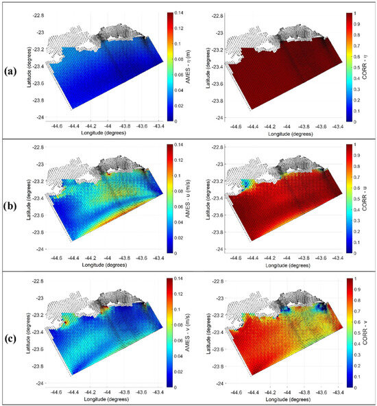
Figure 4.
Spatial distribution of absolute mean error statistic, AMES (on the left), and correlation coefficient—CORR (on the right), for coastal (Delft3D) and ocean (HYCOM) model time series comparison of (a) sea level; (b) zonal current component; and (c) meridional current component. The black dots represent the coastal model computational grid.
There is a strong agreement regarding water levels, as expected, with an AMES below 0.05 and a CORR exceeding 0.98 throughout the entire domain. In the case of currents, we observed more significant disparities at the southern limit, where the flow is parallel to the border, and in the coastal region, close to the mouths of the bays. The latter are due to the ability of the coastal model to simulate flow patterns within bays and their impact on the continental shelf.
Figure 5 presents the five specific points within the domain where both models are compared. The points were selected to represent conditions at different locations within the grid. Two points are situated at the boundaries (P01 and P02), one is in the inner part of the domain (P03), and the remaining two are located at the entrances of the bays (points P04 and P05). The error was calculated for both the total signal and after filtering out the astronomical signal using a 3-day filter.
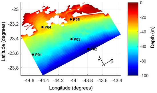
Figure 5.
The geographical locations of compared time series from coastal (Delft3D) and ocean models (HYCOM). The current components (u and v) were decomposed according to the grid orientation.
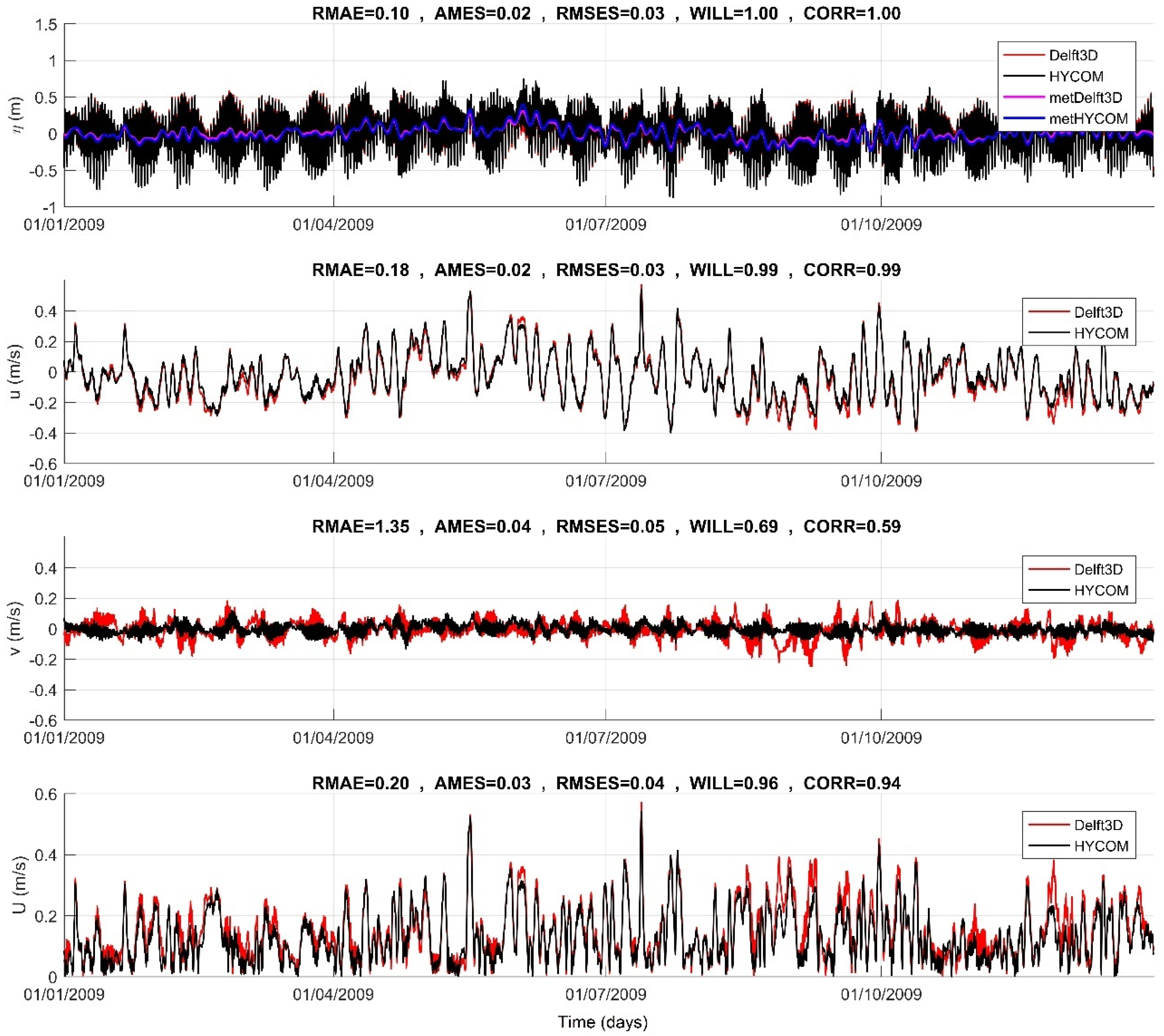
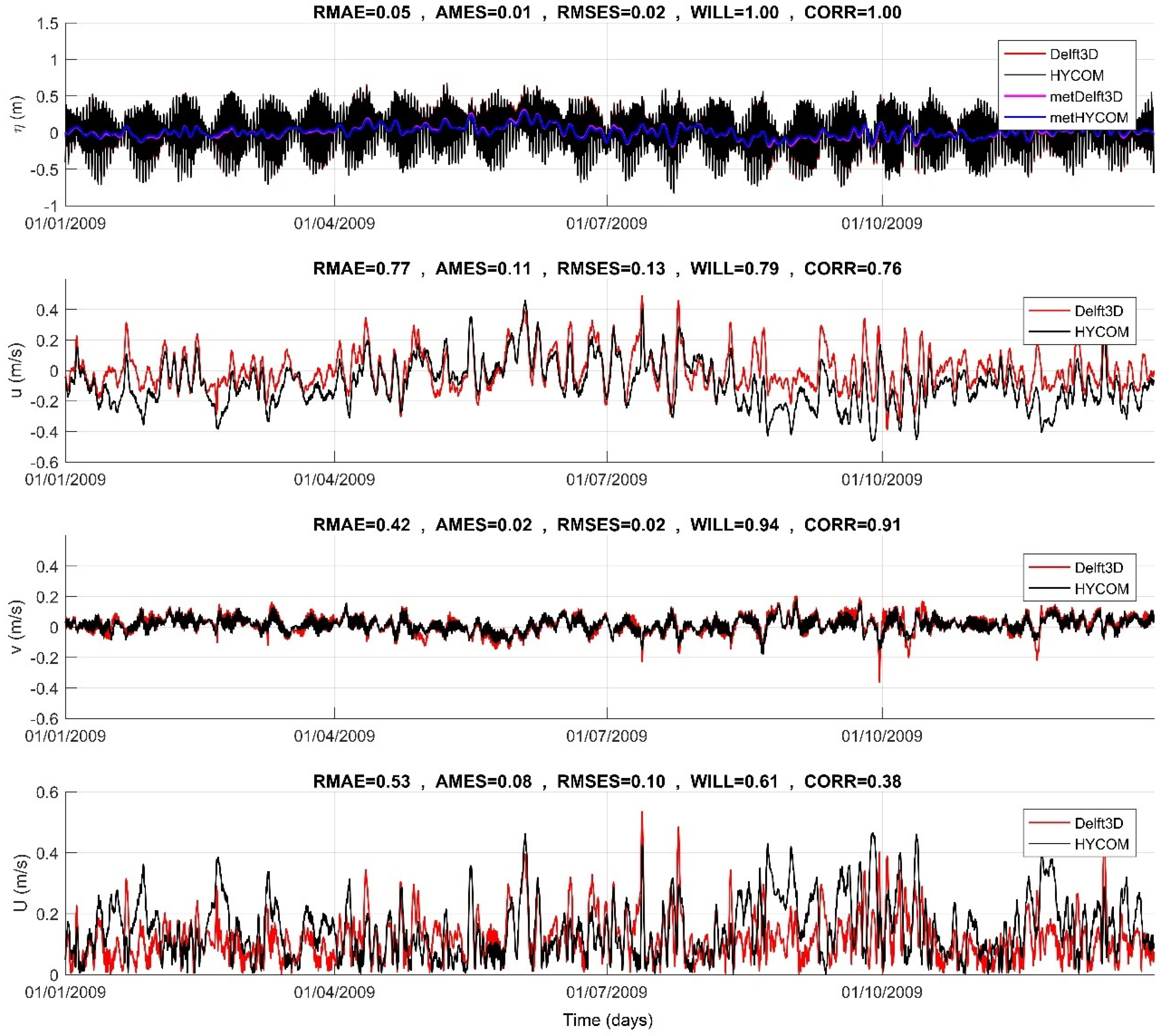
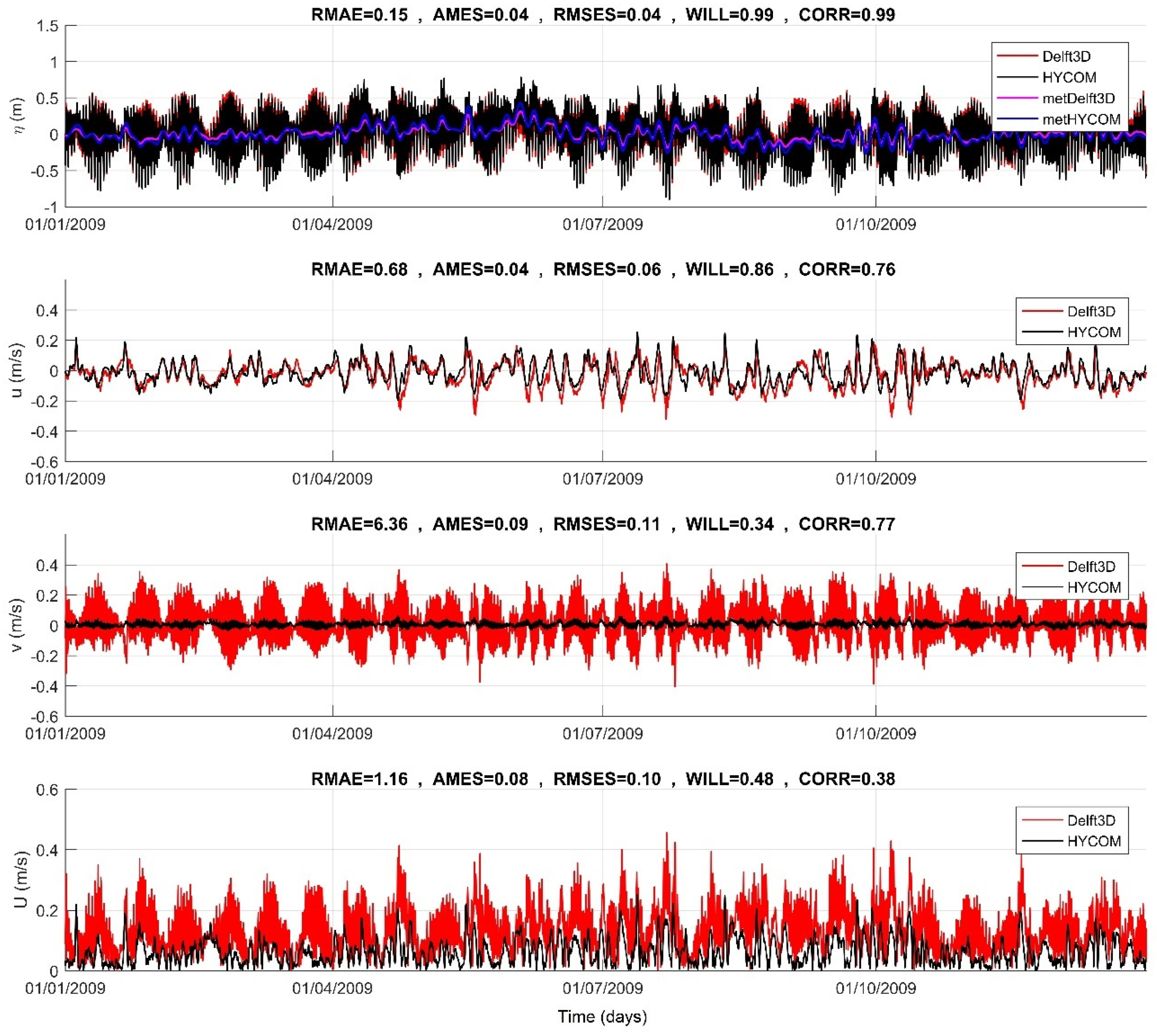
Figure 6, Figure 7, Figure 8 and Figure 9 provide a time series comparison of the results between the coastal and ocean models at four distinct points within the domain, as depicted in Figure 5. Point P01 (Figure 6) is situated at the southern lateral open boundary, where the meteorological flow component is predominantly perpendicular to the boundary. Meanwhile, Point P02 (Figure 7) is located at the ocean boundary, where the meteorological flow component primarily aligns parallel to the boundary. As explained in Equation (2), Riemann’s boundary condition exclusively considers the normal velocity component, potentially leading to more effective data transfer between the models at the southern boundary.
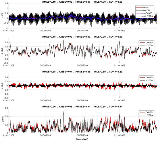
Figure 6.
Comparison between the time series at P01 of the coastal (Delft3D) and ocean models (HYCOM). The series are, from top to bottom, the sea level (η) perpendicular to the boundary current component (u) and parallel to the boundary current component (v) and the current module (U).
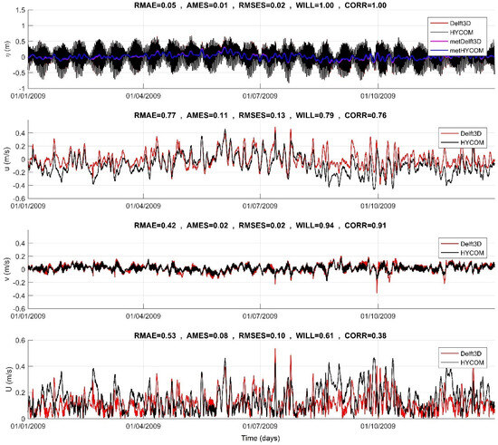
Figure 7.
Comparison between the time series at P02 of the coastal (Delft3D) and ocean models (HYCOM). The series are, from top to bottom, the sea level (η) parallel to the boundary current component (u) and perpendicular to the boundary current component (v) and the current module (U).
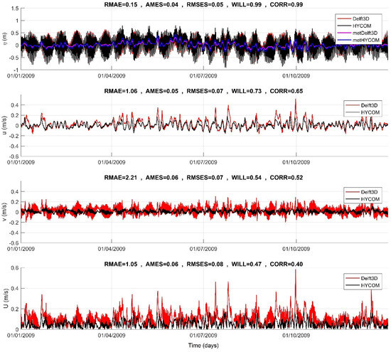
Figure 8.
Comparison between the time series at P04 of the coastal (Delft3D) and ocean models (HYCOM). The series are, from top to bottom, the sea level (η); the along-shelf current component (u); the cross-shelf current component (v); and the current module (U).

Figure 9.
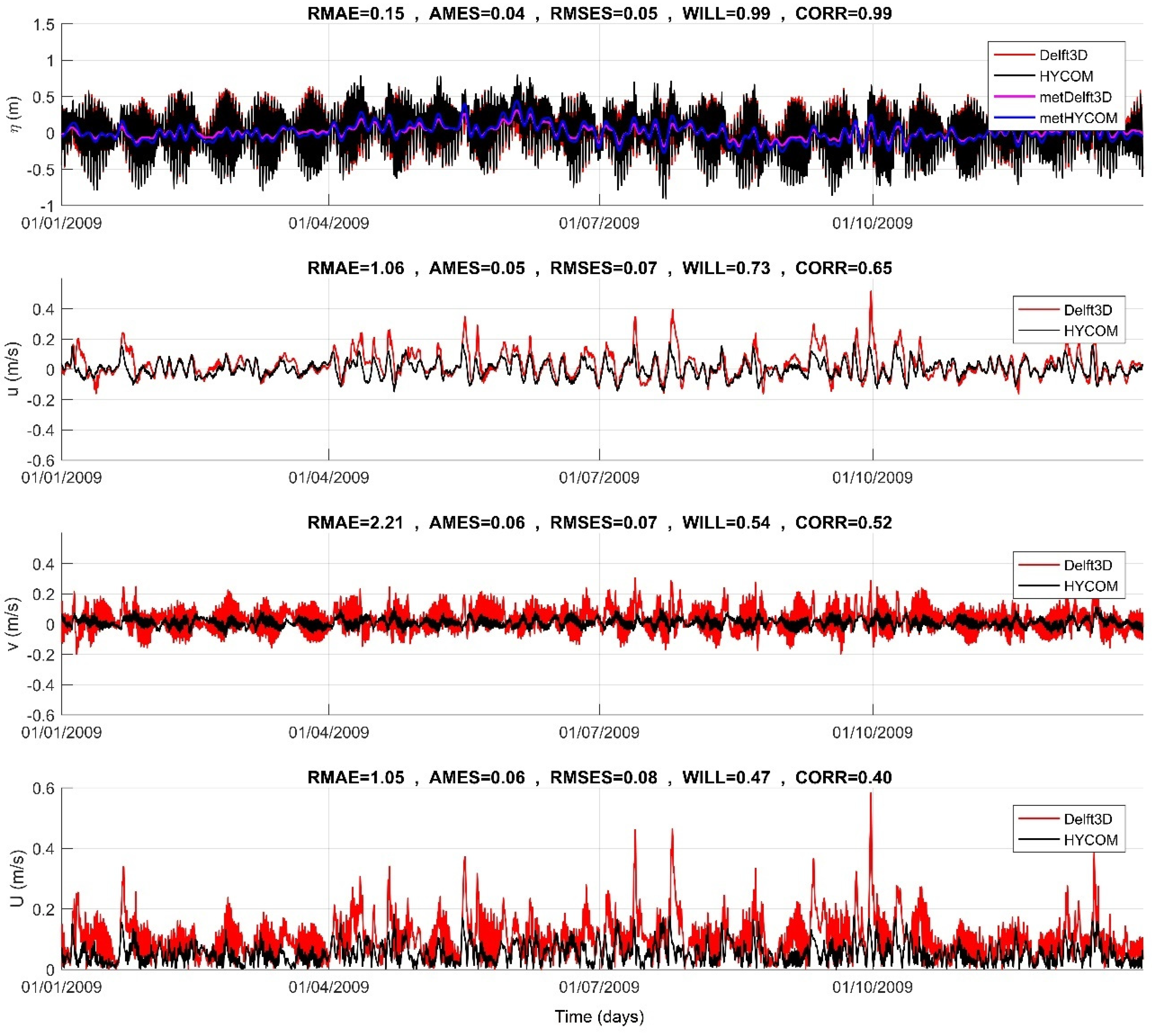
Comparison between the time series at P05 of the coastal (Delft3D) and ocean models (HYCOM). The series are, from top to bottom, the sea level (η); the along-shelf current component (u); the cross-shelf current component (v); and the current module (U).
At Points P04 (depicted in Figure 8) and P05 (illustrated in Figure 9), situated at the entrances of Ilha Grande Bay and Sepetiba Bay, respectively, a pronounced coastal parallel flow induced by meteorological factors is evident. However, it is noteworthy that the current component (v) entering the bays exhibits a notably strong astronomical influence in the currents modeled within the coastal framework, surpassing that observed in the ocean model. This disparity can be attributed to the poor inner bay representations in the ocean model, as visually indicated by the grid overlap shown in Figure 1. It is important to highlight that when a larger area of the bays is included in the model grid, the resulting tidal currents will show higher magnitudes, as occurred in the coastal model. This is primarily because of the improved representation of the tidal prism.
The flow component that runs perpendicular to the boundaries, such as the u component at point P01 and the v component at point P02, exhibits relatively low error values when compared to the parallel flow component. As previously mentioned, Riemann’s boundary condition fails to capture information about the flow parallel to the boundary. At P01, the meteorological signal, which is predominantly found in the u component, is represented with minimal relative or absolute errors. However, it is important to note the suboptimal representation of the astronomical flow signal at this boundary, which is primarily present in the v component.
In contrast, at P02, where the astronomical flow component is mostly perpendicular to the boundary (the v component), it is well represented in the nesting. The meteorological flow, which is parallel to this boundary, is also better represented than its counterpart at P01, driven by tidal forces.
Moving to Points P04 and P05 located at the bay entrances, larger errors are observed in the v component due to the ocean model’s limitations in accurately representing tidal flows. In Sepetiba Bay, where the tidal flow is particularly strong due to its propagation in the elongated bay, more significant differences are noticeable.
It is of paramount importance to underscore the significant differences in the computational grids used in the two models, particularly in the coastal region. The HYCOM simulations used in this work, which provide boundary conditions for the coastal model (Delft3D), fall short of capturing the intricate geographical features of Ilha Grande Bay and Sepetiba Bay, as well as the connection between Sepetiba Bay and the sea via the eastern channel known as “Bacalhau” (as depicted in Figure 3). This lack of detailed geometry significantly hinders the accurate simulation of the robust flood and ebb currents that are characteristic of this area. Moreover, the transmission of tidal signals in water levels from the ocean model to the open boundary of the coastal model enables their propagation into the interior of the bays and connections, a dynamic not replicated in the larger-scale model.
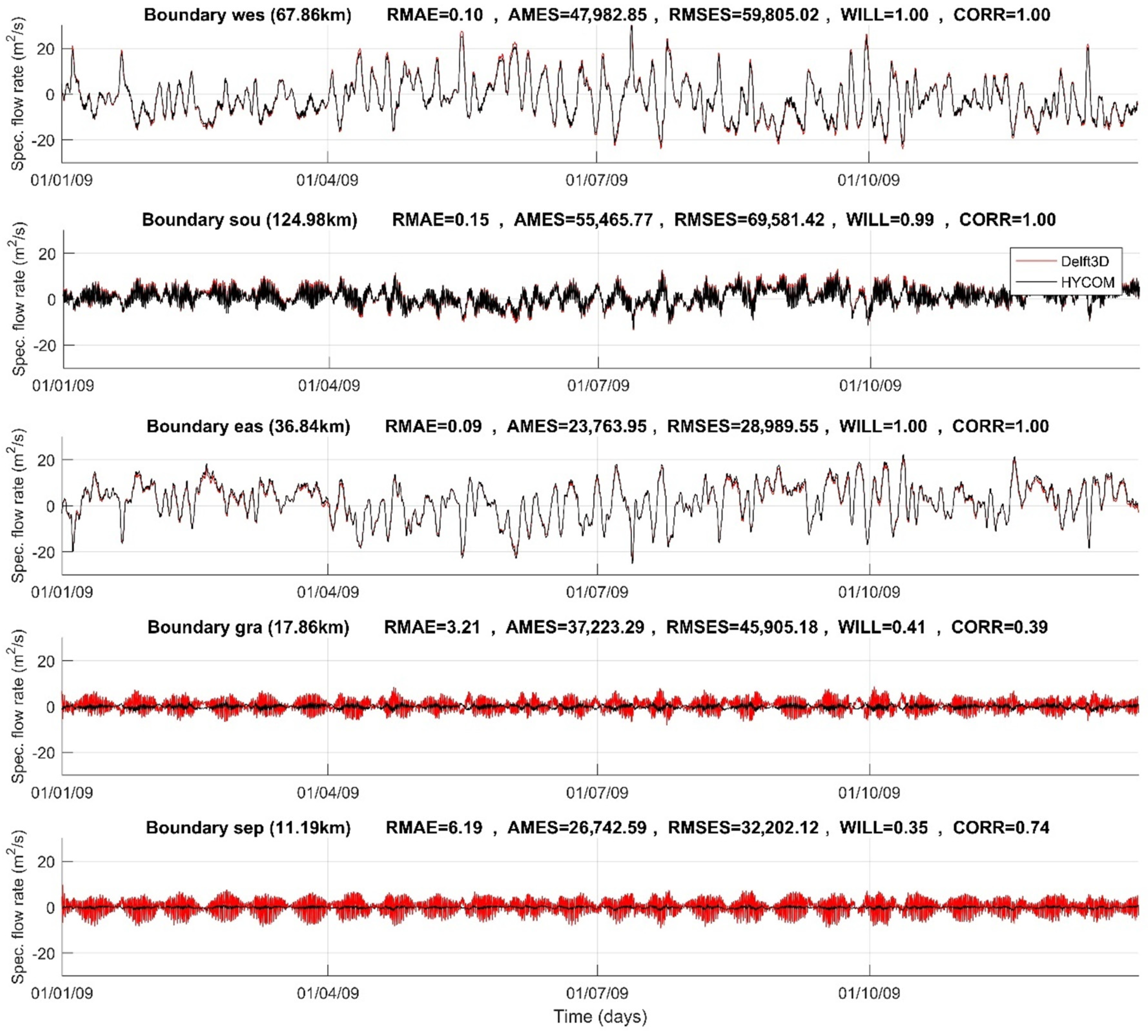
An alternative method for measuring the nesting effects involves examining the flow rates along the boundaries. Positive flow rates indicate an outward direction from the control volume. At both the western (where P01 is situated) and eastern boundaries, meteorological forcing predominantly influences the flow rates, with specific flow rates being comparable, as revealed in Figure 10. Along the southern boundary (where P02 is located), the flow rate is significantly shaped by the onshore–offshore tidal flow, with specific flow rates approximately half the intensity observed along the western and eastern boundaries. As anticipated, at Points P04 and P05, situated at the entrances of the bays (gra and sep), the flow rates are also substantially dictated by the tidal dynamics, with a slightly greater impact of meteorological forcing observed in Ilha Grande Bay (gra).
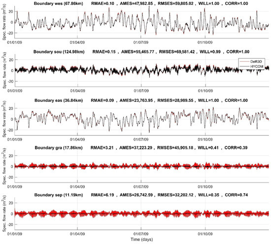
Figure 10.
Comparison between the time series of specific flow rate for the coastal (Delft3D) and ocean (HYCOM) models at the boundaries: wes (where P01 is located), sou (where P02 is located), and eas, closing the domain, and at the entrances of Ilha Grande Bay (gra) and Sepetiba Bay (sep).
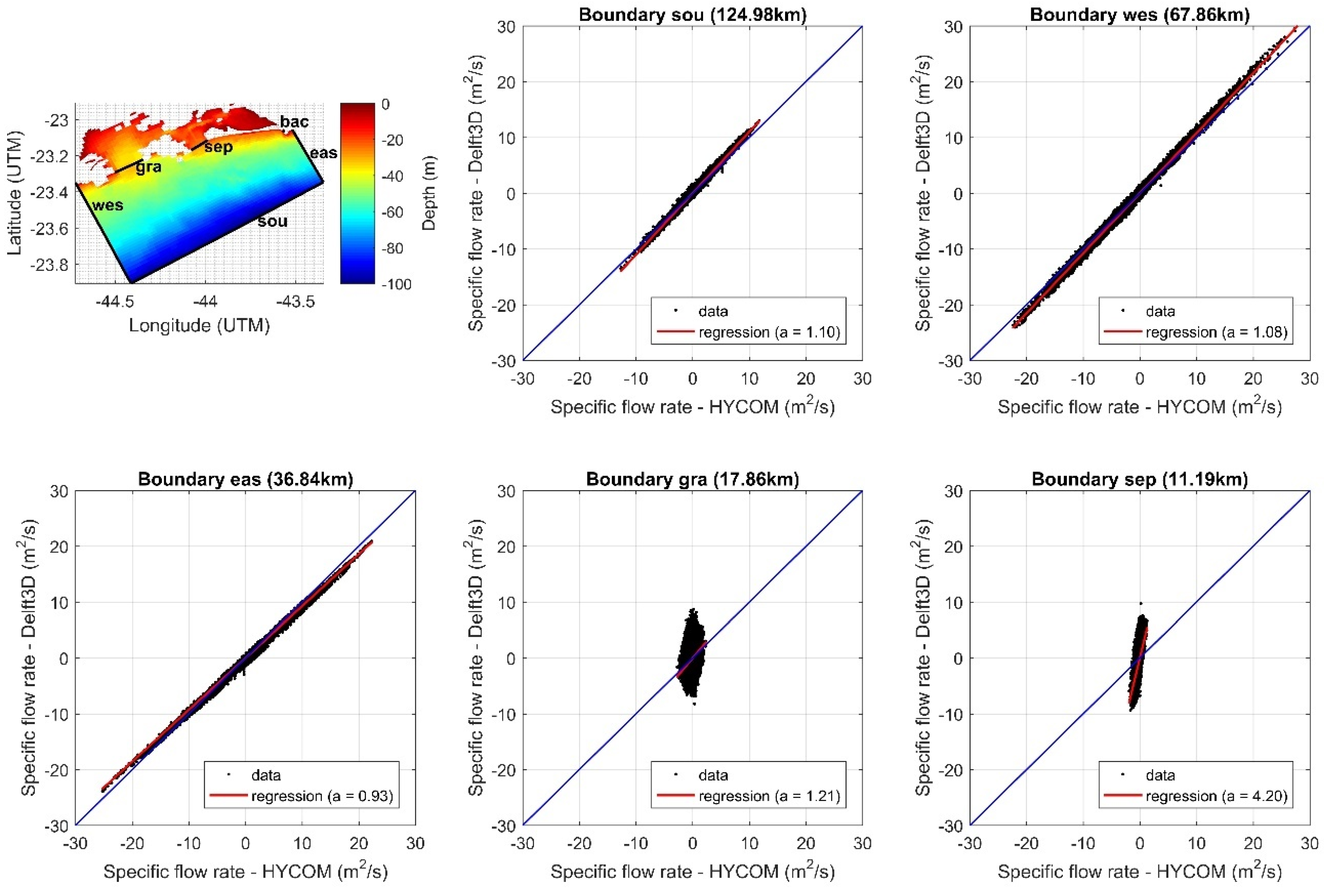
In Figure 11, a linear regression analysis is presented, comparing the time series data from the coastal model (Delft3D) and the ocean model (HYCOM). Along the western (wes), southern (sou), and eastern (eas) ocean boundaries, the angular coefficients are 1.08, 1.10, and 0.93, respectively. These coefficients suggest a slight overestimation by the coastal model of the flow along the western and southern boundaries and an underestimation along the eastern boundary. However, at the entrances to the bays, particularly Ilha Grande Bay (gra) and Sepetiba (sep) Bay, the angular coefficients are notably larger, measuring 1.21 and 4.2, respectively. As previously discussed, tidal influence dominates the flow patterns at these locations. Consequently, in the coastal model, a more accurate description of the coastal geometry and bathymetry and the inclusion of bays result in an enhancement in the tidal prism representation.

Figure 11.
Linear regression of the specific flow rate time series of the coastal (Delft3D) and ocean (HYCOM) models at the boundaries: western—wes (where P01 is located), southern—sou (where P02 is located), and eastern—eas, closing the domain, and at the entrances of Ilha Grande Bay (gra) and Sepetiba Bay (sep).
Table 1 and Table 2 provide insights into the volumes of water crossing the boundaries over the simulation year. Both models exhibit a minor loss of mass, amounting to 0.30% for the ocean model and 0.41% for the coastal model. However, significant disparities emerge when comparing the volume of water crossing these boundaries between the two models. The differences between the models in terms of the volume traversing the boundaries vary considerably, with a −0.52% variation observed at the western boundary, a substantial 7.79% and −6.27% contrast at the southern and eastern boundaries, respectively, and discrepancies of 82.25% and 97.19% at the mouth of the bays.

Table 1.
Total water volumes crossing the boundaries for the coastal (Delft3D) and ocean (HYCOM) models.

Table 2.
Initial and final volumes in the domain for the coastal (Delft3D) and ocean (HYCOM) models.
3.2. Comparison of Water Level Signal with Available Data
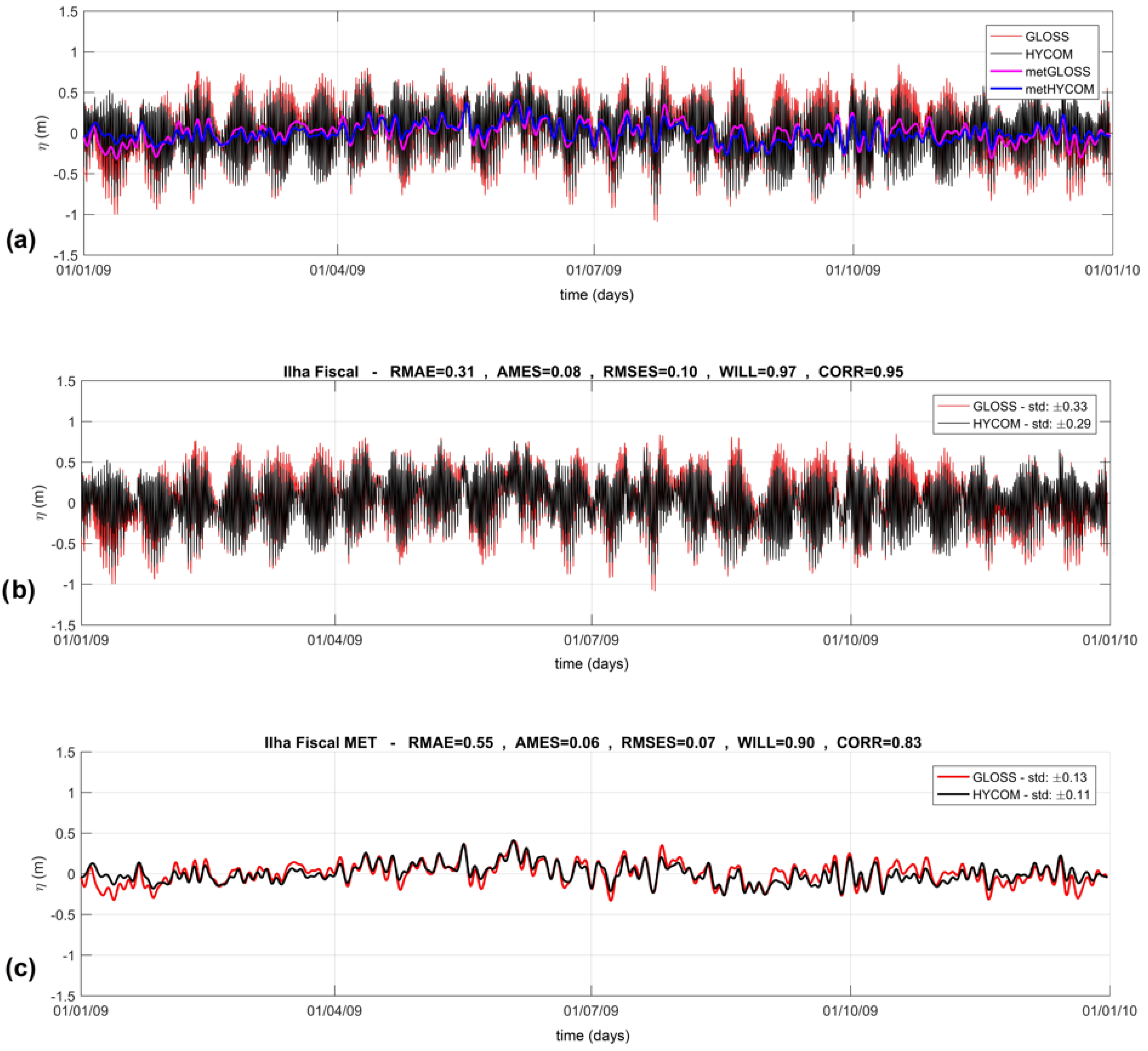
To validate the outcomes of the ocean model, the HYCOM, a comparison of the sea level time series was conducted, encompassing the entire dataset and considering astronomical and non-astronomical signals. We compared Fiscal Island gauge station data (as shown in Figure 12) with the model results obtained at the entrance of Guanabara Bay (as illustrated in Figure 1).
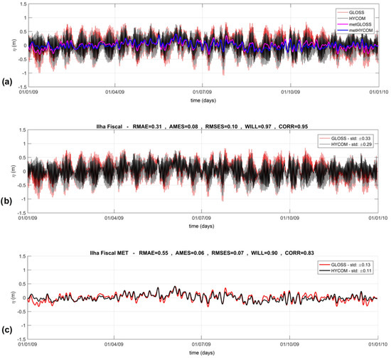
Figure 12.
Comparison of sea level time series from the ocean model, HYCOM, and data in Guanabara Bay considering: (a) complete signal and time series after removal of the astronomical signal; (b) only the astronomical signal; and (c) only the non-astronomical signal.
An examination of the results reveals an underestimation of the sea level amplitude by the model, a trend that is notably less pronounced during the winter period. This underestimation is substantiated by both absolute and relative error metrics. Nonetheless, the high values of the correlation coefficient and Willmott parameter for both astronomical and non-astronomical signals point to a robust agreement between the model and the observed data, despite the observed underestimation of the sea level amplitude.
The Southeastern Brazilian Continental Shelf exhibits a highly barotropic response to low-frequency wind forcing, as demonstrated by Stech and Lorenzzetti [64]. Previous studies by Zamudio et al. [65] and Gabioux et al. [44] have highlighted some underestimation in the sea level’s amplitude when simulating coastal trapped waves using the HYCOM, with differences in sea levels of approximately 0.15 m.
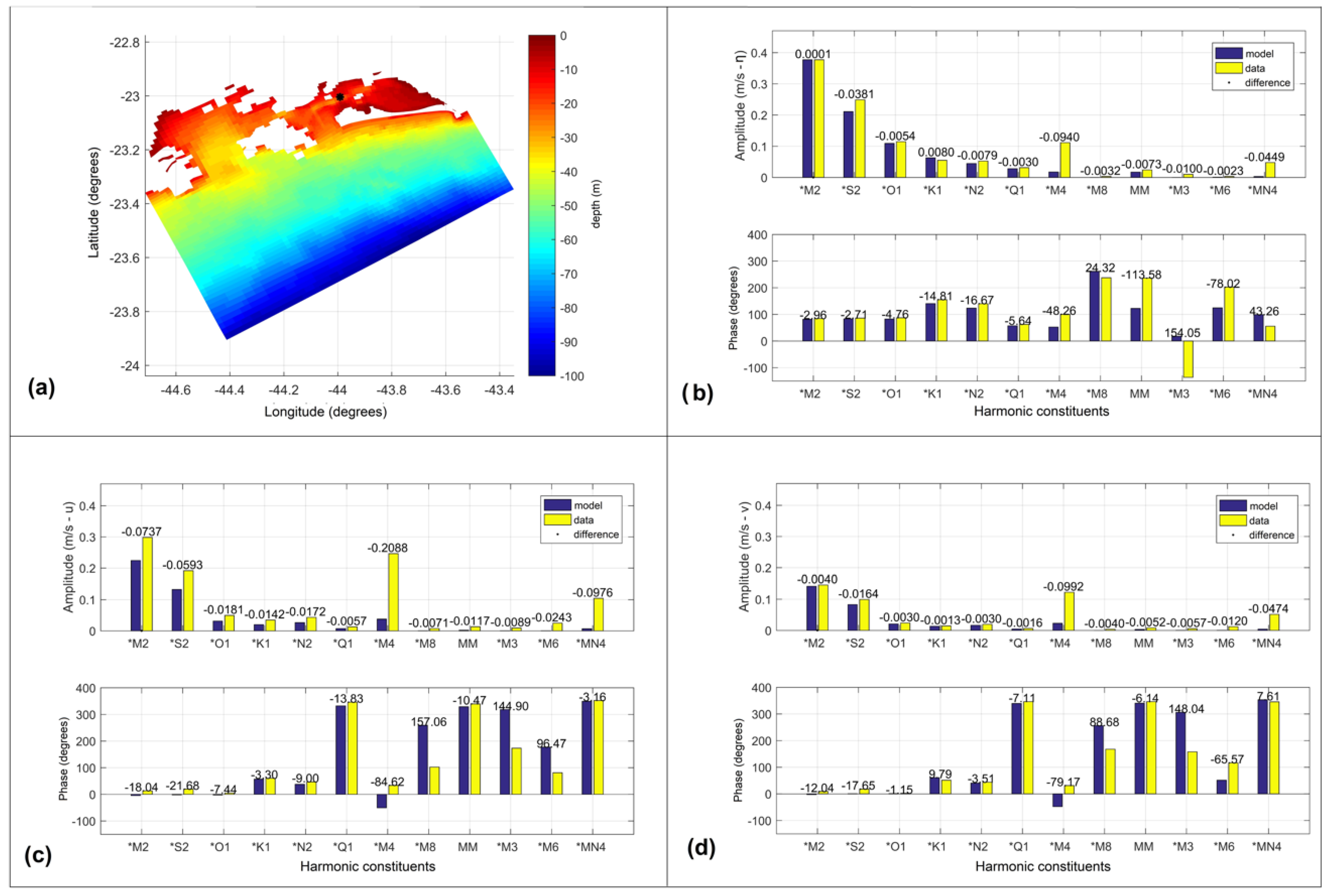
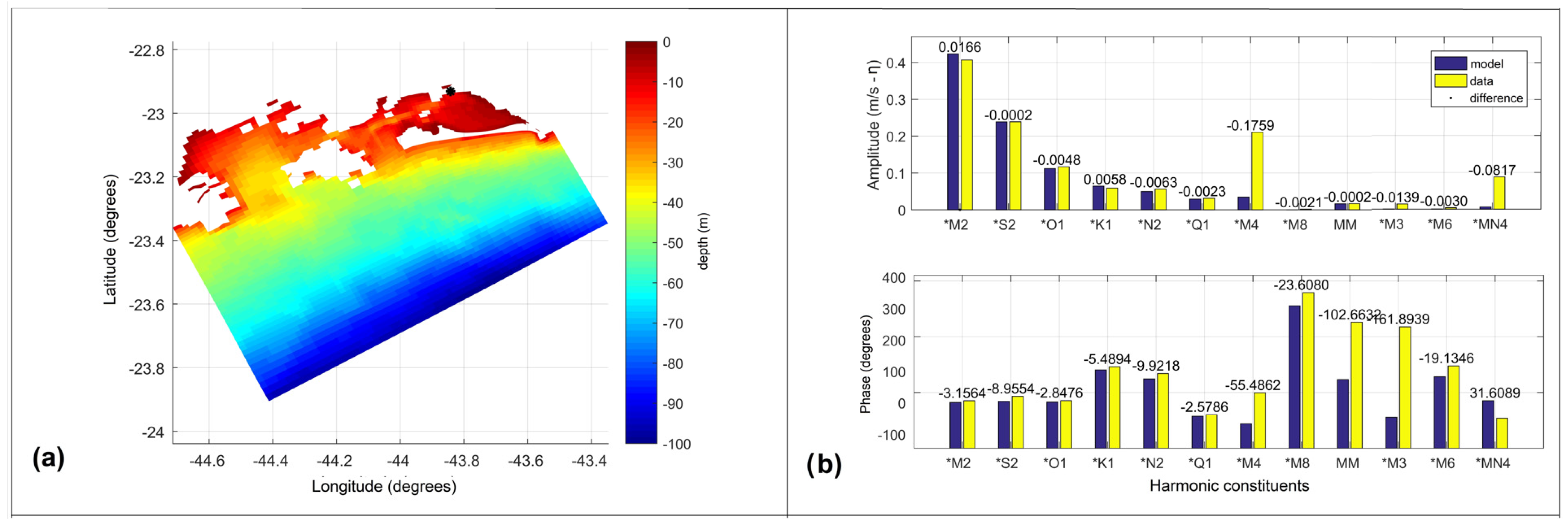
The performance of the coastal model was assessed with a focus on tidal forcing when confronted with monitoring stations data. The astronomical components of the model results were compared to the corresponding astronomical components obtained from the data set at Ilha Guaíba station for both water levels and currents (Figure 13), as well as at the Port of Itaguaí station, exclusively for water levels (Figure 14). Both points are located within Spetiba Bay, which, as pointed out by Signorini [33,34], has hydrodynamics marked by a strong tidal circulation, being the largest in the region according to Harari and Camargo [39], with large M2 and S2 components.
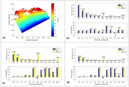
Figure 13.
Ilha Guaíba station: (a) location. Amplitude and phase histograms for measured data and coastal model results: (b) sea water level tidal components, (c) zonal current tidal components, and (d) meridional current tidal components. Also shown in the graph are the (*) difference between the results of the model and the monitoring station data.

Figure 14.
Itaguaí Port station: (a) location and (b) comparison of amplitude and phase histograms for measured data and coastal model results for sea water level tidal components. Also shown in the graph are the (*) difference between the results of the model and the monitoring station data.
It is worth noting that Teixeira et al. [66] previously observed similar discrepancies when comparing astronomical component data across time series of varying lengths, encompassing different periods of the year. According to these authors, these discrepancies tend to exponentially decrease as the length of the time series used for the comparison increases. In the context of currents, the coastal model tends to exhibit larger differences, often resulting in an underestimation of amplitudes. Additionally, the shallow-water tidal constituents generally display underestimated amplitude values, an outcome that can be expected given that the HYCOM incorporates only the eight primary harmonic components [29]. Pairaud et al. [67] highlighted the necessity of prescribing deep ocean boundary conditions for the M4 tidal constituent in ocean models.
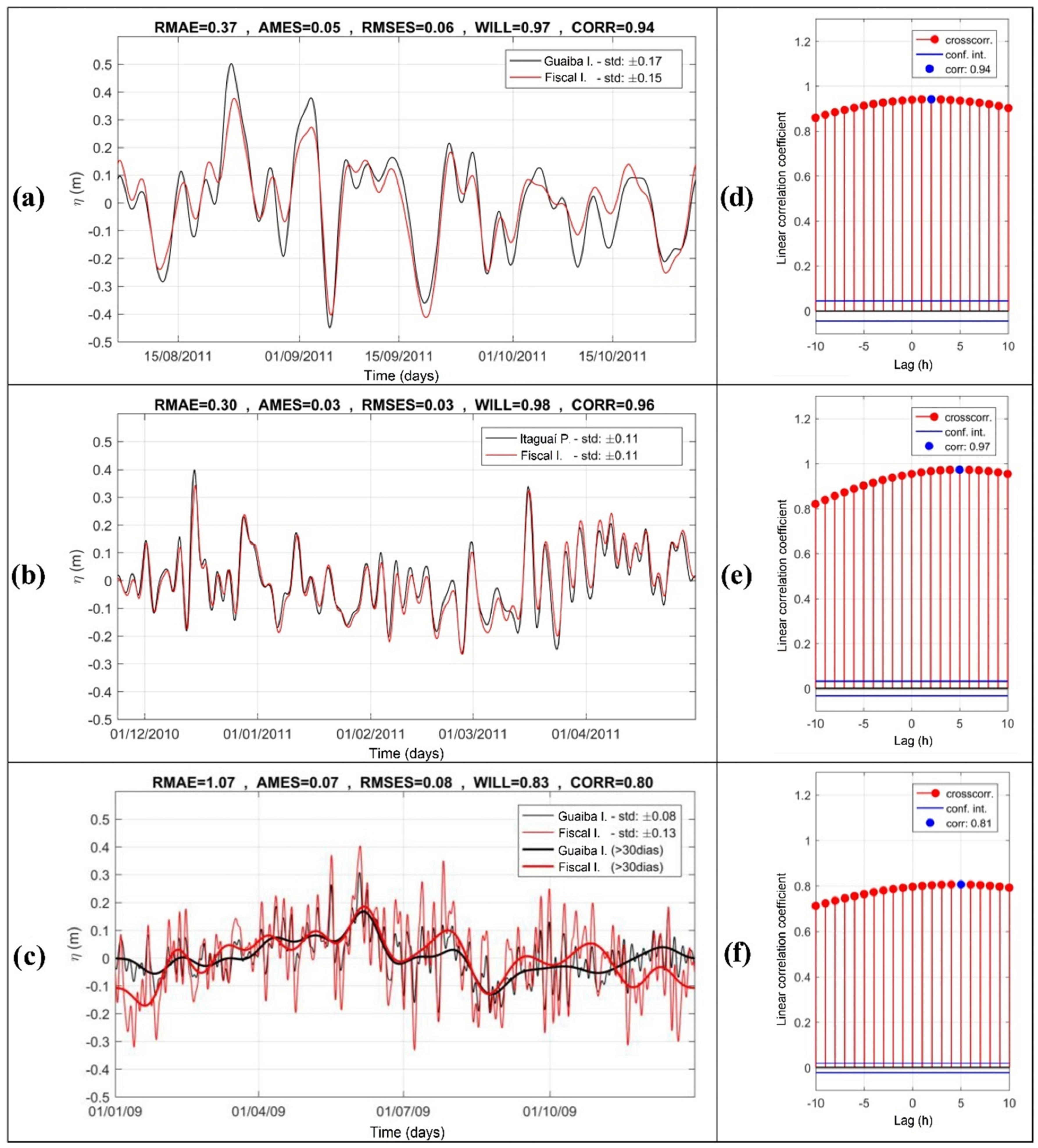
In the first two panels of Figure 15, we compare sea level measurements from the Guaíba Island station (a) and the Itaguaí Port station (b), both situated in Sepetiba Bay, with sea level measurements from the Fiscal Island gauge station in Guanabara Bay. This comparison is made after the removal of astronomical components. As previously discussed, a coastal trapped wave, induced by remote meteorological forces, travels from the southern to the northern Brazilian Continental Shelf. This wave’s propagation velocity changes in accordance with the region’s geometry, gradually diminishing in amplitude from south to north. The time taken for the coastal trapped wave to propagate from Sepetiba to Guanabara Bay (as shown in Figure 2) was derived from available data and numerical simulations.
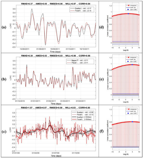
Figure 15.
Comparison of sea level measurements in Guanabara Bay (Fiscal Island station) and Sepetiba Bay, (a) Guaíba Island station, and (b) Port of Itaguaí station and time lags from correlations (d) and (e), respectively. (c) Comparison between model results and sea level measurements. Data from Guanabara Bay (Fiscal Island station) and modeled sea levels in Sepetiba Bay (Guaíba Island station) and corresponding time lag for 2009 time series, and (f) is the time lags from this correlation. All cases after astronomical component removal. After removing lower-than-30-day components in the lower panel, the annual seasonality is highlighted for the 2009 time series.
Figure 15a,b depict time series and correlation coefficients, while Figure 15d,e showcase the respective time lags between these series. For the Guaíba Island station, the time lag is approximately 2 h, whereas for the Guaíba Itaguai Port station, it extends to 5 h. This is coupled with a higher correlation, indicating that the coastal trapped wave is moving northward in both cases.
Moving to the third panel of Figure 15c, we compare the modeling results to measurements after the removal of astronomical components for the entire simulated year of 2009. The data were collected from the Fiscal Island gauge station in Guanabara Bay, and the modeling results for Sepetiba Bay were obtained at the Guaíba station. As expected, the correlations among the series are notably lower, but the primary characteristics are well represented. In the context of the meteorological signal’s seasonality, a 30-day low-pass filter is also presented in Figure 15c. The numerical simulations closely follow the annual pattern observed by Campos et al. [68], who analyzed observations from the Port of Santos in São Paulo, revealing a higher number of positive extremes (40.2%) in autumn and a greater number of negative extremes (47.2%) in spring. A similar pattern is observed by Kjerfve et al. [35] in their observations from the Ilha Grande Channel.
Table 3 presents the maximum cross-correlation and time lag values across various time periods. For long time series, it tends to stabilize around a 5 h time lag. The propagation speed averages approximately 5 m/s. Notably, this value is significantly lower than the coastal wave propagation speed of 12.2 m/s observed from Imbituba to Sepetiba Bay (as illustrated in Figure 3), which is situated 748 km south and exhibits a time lag of 17 h with a cross-correlation of 0.83. These findings are consistent with previous research conducted by Castro and Lee [28], França [29], and Dottori and Castro [30].

Table 3.
Maximum cross-correlations and corresponding time lags of measured sea water levels in Guanabara Bay (Ilha Fiscal station) and modeled for Sepetiba Bay (Guaíba Island station) after astronomical component removal.
As suggested by Melo Filho [17], the reduction in propagation speed can be attributed to the narrowing of the Brazilian Continental Shelf, a notion similarly emphasized by Brink [24] and Platov [11]. In the southern region, between Imbituba and Sepetiba Bay, the Continental Shelf width, extending from the coast to the 200 m isobath, spans approximately 200 km. However, between Sepetiba Bay and Ilha Fiscal, this width is approximately halved, measuring roughly 100 km. This phenomenon is a result of energy dissipation due to bottom friction, as noted by Gutiérrez et al. [69], and the significant dispersion of energy between wave propagation modes in stratified ocean conditions, as highlighted by Wilkin and Chapman [70].
The standard deviation of the sea level varies between ±0.11 m and ±0.17 m, with lower values recorded during the autumn season (as shown in Figure 15a,b) in Sepetiba Bay. Similarly, measurements in Guanabara Bay for the year 2009 exhibit a comparable standard deviation of ±0.13 m (as depicted in Figure 15c). Notably, the numerical results from the ocean model (the HYCOM) show a slightly lower sea level standard deviation of ±0.11 m, indicating an underestimation of the meteorological signal. This observation aligns with findings reported by França [29], Carvalho [56], and Daher et al. [71].
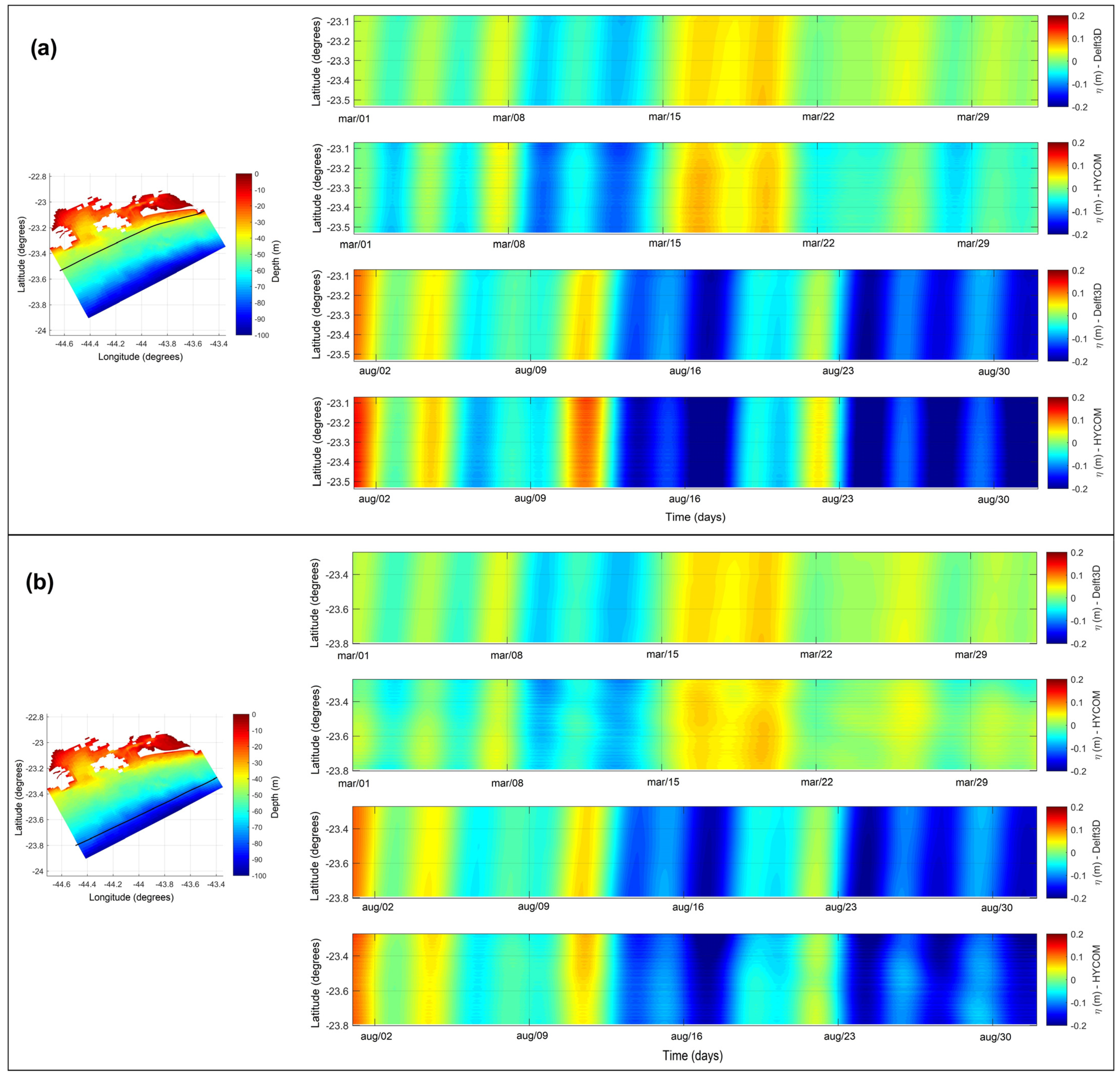
Figure 16 provides a comparative analysis of the temporal variability in sea level, with the astronomical signal removed, using a 3-day filter for water level data for the year 2009. This comparison is made between the ocean model (the HYCOM) and the coastal model (Delft3D). Two transects are illustrated: one situated closer to the coastline at a depth of approximately 50 m (a) and another farther offshore at approximately 80 m in depth (b). The results are presented for two scenarios: the first represents a less intense meteorological signal observed in March (upper panels), and the second depicts a stronger meteorological signal observed in August (lower panels). The temporal evolution along the transect, indicated by the latitude, displays the propagation of the meteorological wave towards the north.
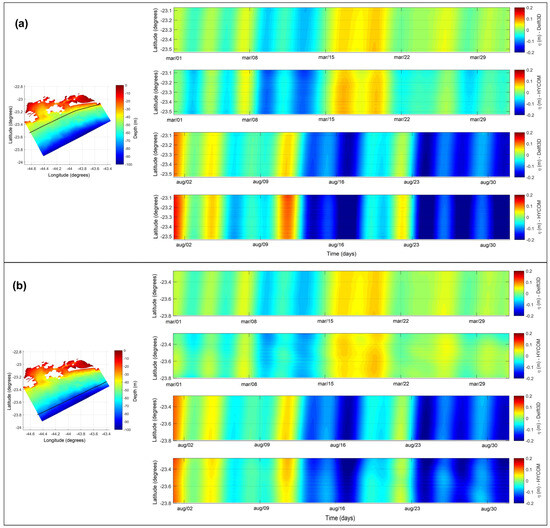
Figure 16.
Comparison of HYCOM and Delft3D model results after removing the astronomical signal. Temporal variability of sea water level along two coastal transects (a) near and (b) far from the coastline. Results for the months of March/2009 (upper panels) and August/2009 (lower panels). The x in magenta is the center point of the transects.
At a point along the deeper transect (magenta dot in Figure 16), both models exhibit a similar standard deviation of ±0.08 m near the boundary. However, when we examine a point in the shallower transect (magenta x in Figure 16), we observe that the standard deviation of sea level is ±0.08 m for Delft3D and ±0.11 m for the HYCOM. This discrepancy indicates an attenuation of the meteorological signal near the coast after employing the coastal model nesting, resulting in a loss of signal amplitude in comparison to the ocean model.
3.3. Spatial Analysis of Tidal and Non-Tidal Signals
To gain a deeper understanding of the patterns associated with tidal and non-tidal signals driven by meteorological forces, we first examined the results from the simulation of coupled models, encompassing both S1 and S2 scenarios. We focused on the spatial distribution of the amplitude and phase of the astronomical constituent M2, with reference to the simulation that considers the outcome of the HYCOM model (as depicted in Figure 17a).
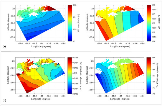
Figure 17.
Amplitude (on the left) and phase (on the right) of the M2 tidal constituent (a) and the period of 4.73 days of the meteorological signal (b) from the time series of simulations in Delft3 considering the coupling of results from the HYCOM.
Our results revealed a southward phase propagation, consistent with the findings of Harari and Camargo [39] for the majority of the primary tidal constituents. Notably, the phase difference between the two ends of the boundary parallel to the coastline is relatively small, measuring nearly 4 degrees. As we approach the entrances of the bays, this phase aligns itself parallel to these entrances, progressing further inland in phase at the two main entry points and amplifying its effect as it moves deeper into Sepetiba Bay. This phase propagation aligns with Signorini’s [34] observations of tidal signals propagating in phase within the estuarine system’s primary entrances.
The amplitude isolines exhibit a nearly perpendicular orientation to the coast, indicating similar amplitudes at the primary system entry points and amplification as they progress further inland within the system.
Regarding the constituent with a period of 4.73 days, representing the meteorological signal (as illustrated in Figure 17b), our observations revealed a phase propagation toward the northeast, consistent with the findings of Castro and Lee [28]. A significant phase difference exists between the two ends of the boundary parallel to the coast, amounting to nearly 30 degrees. This phase difference is less pronounced within Sepetiba Bay but becomes more prominent in the channel between Ilha Grande and the mainland. The amplitude of this signal demonstrates a correlation with the phase, with greater amplitudes observed in Ilha Grande Bay, accompanied by a more pronounced level gradient in the channel between the bays. It is worth noting that the amplitudes of this signal are notably smaller when compared to M2.
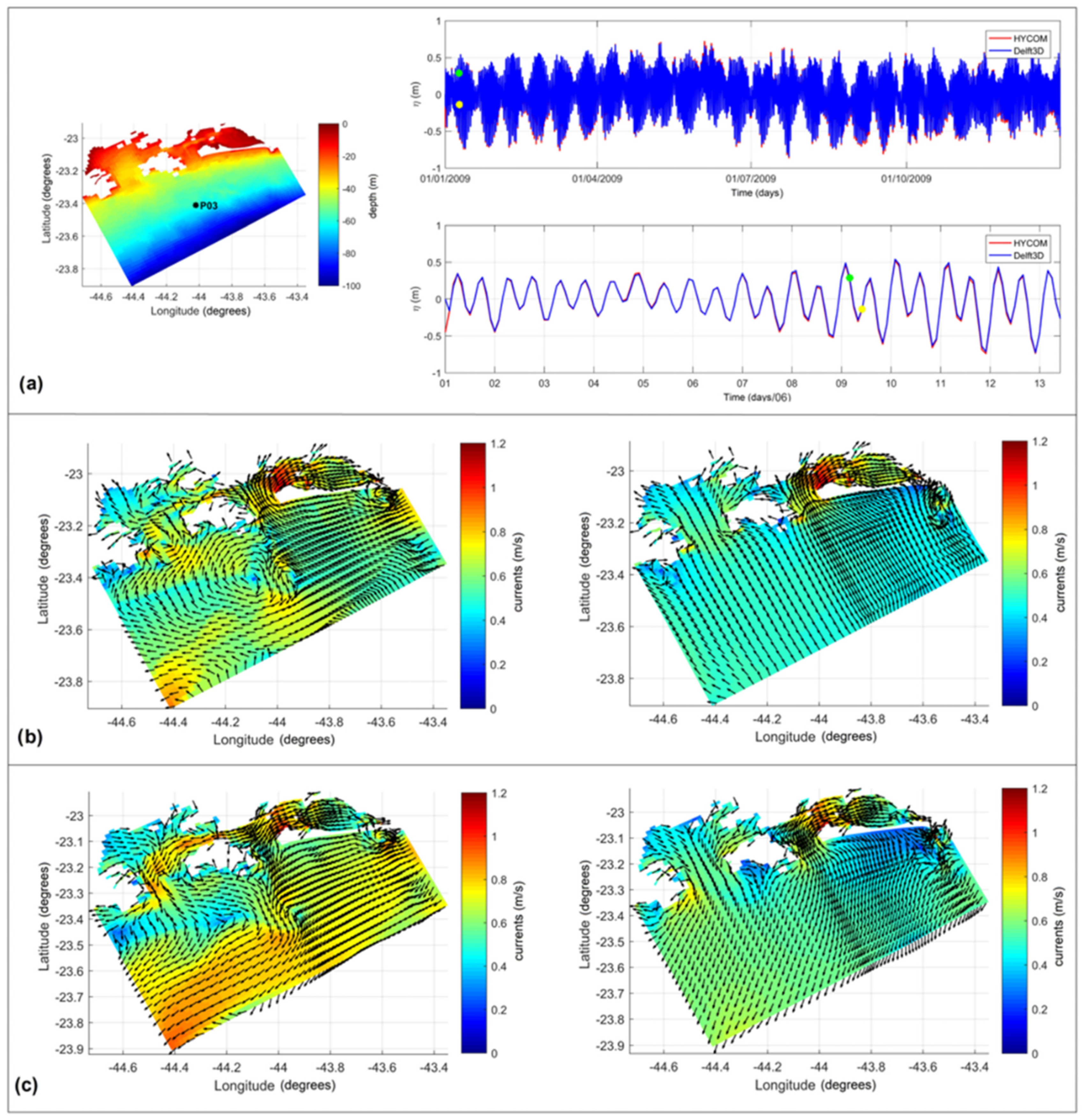
In the spatial distribution of our simulation results, illustrated on the right side of Figure 18b,c, a stronger tidal forcing is evident in Sepetiba Bay compared to Ilha Grande Bay, both during flooding and ebbing tides, as shown by Mordente [72].

Figure 18.
Comparison between Delft3D and HYCOM time series (a, on the right) for a central point in the computational mesh (a, on the left), focusing on the moments of flood (yellow dot) and ebb (green dot) used in the spatial representation of the Delft3D results with (on the left) and without (on the right) the meteorological signal for instants of flood (b) and ebb tides (c).
The spatial distribution of the simulation, focusing solely on astronomical effects (S2 scenario), exhibits a similarity in the flood and ebb patterns within the interior of Sepetiba Bay. However, in Ilha Grande Bay and the surrounding marine areas, these patterns differ significantly, both in terms of intensity and direction. At this moment, the currents flow to the southwest, aligning with the passage of the meteorological signal.
This spatial pattern aligns with prior research findings [36,37,73]. It is evident that flood currents within Sepetiba Bay are more intense than ebb currents, a phenomenon also observed in Ilha Grande Bay, as highlighted by Fragoso [36] and Cavalcante [37]. This pattern underscores the significant influence of tides on circulation in Sepetiba Bay compared to Ilha Grande Bay, an observation in line with Signorini’s [33] research.
The spatial distribution of the mean values of the differences in the fields of speed and water levels of the two simulations, without and with the weather tide, is shown in Figure 19. All values are negative in the entire domain, for the water level and for the currents, meaning that the scenario that does not take into account the meteorological signal at the sea level underestimates the sea level and the currents, varying spatially.

Figure 19.
Spatial distribution of the mean difference between the time series of the Delft3D results with and without the meteorological signal for sea level (left) and current intensity (right). Differences were computed point to point for the whole year.
In the interior of the bays, in relation to the levels, the greatest differences are observed at the east ends, for Sepetiba Bay, and west, for Ilha Grande Bay. These differences may be the reason for the intensification of the currents in the canal. With regard to the currents, the greatest differences occur precisely along the channel, with differences of the order of 0.2 m/s. Inside the Bay of Sepetiba, the differences are reduced (near to zero), demonstrating the dominance of the astronomical tide in the generation of currents when compared with Ilha Grande Bay. In much of Ilha Grande Bay, the differences in currents exceed 0.1 m/s. On the continental shelf, the current field is dominated by the meteorological signal, with a uniform underestimation of the order of 0.2 m/s (at average values).
In a study by Signorini [34], simulations were conducted to investigate the effects of phase lag on open boundaries for tidal signals (M2, S2, and M4). It was observed that no phase lag resulted in very low currents in Ilha Grande Channel (approximately 0.04 to 0.05 m/s). However, the introduction of a phase lag (20 min) along the boundary led to an intensification of currents in Ilha Grande Channel, reaching around 0.20 m/s with alternating flow directions. Nevertheless, this scenario did not align with the in situ data analyzed by the author. Nonetheless, this experiment emphasized that the presence of a lag in open boundary sea levels could be a crucial factor in understanding the intensification of currents in Ilha Grande Channel, owing to the generation of a barotropic pressure gradient resulting from sea level disparities.
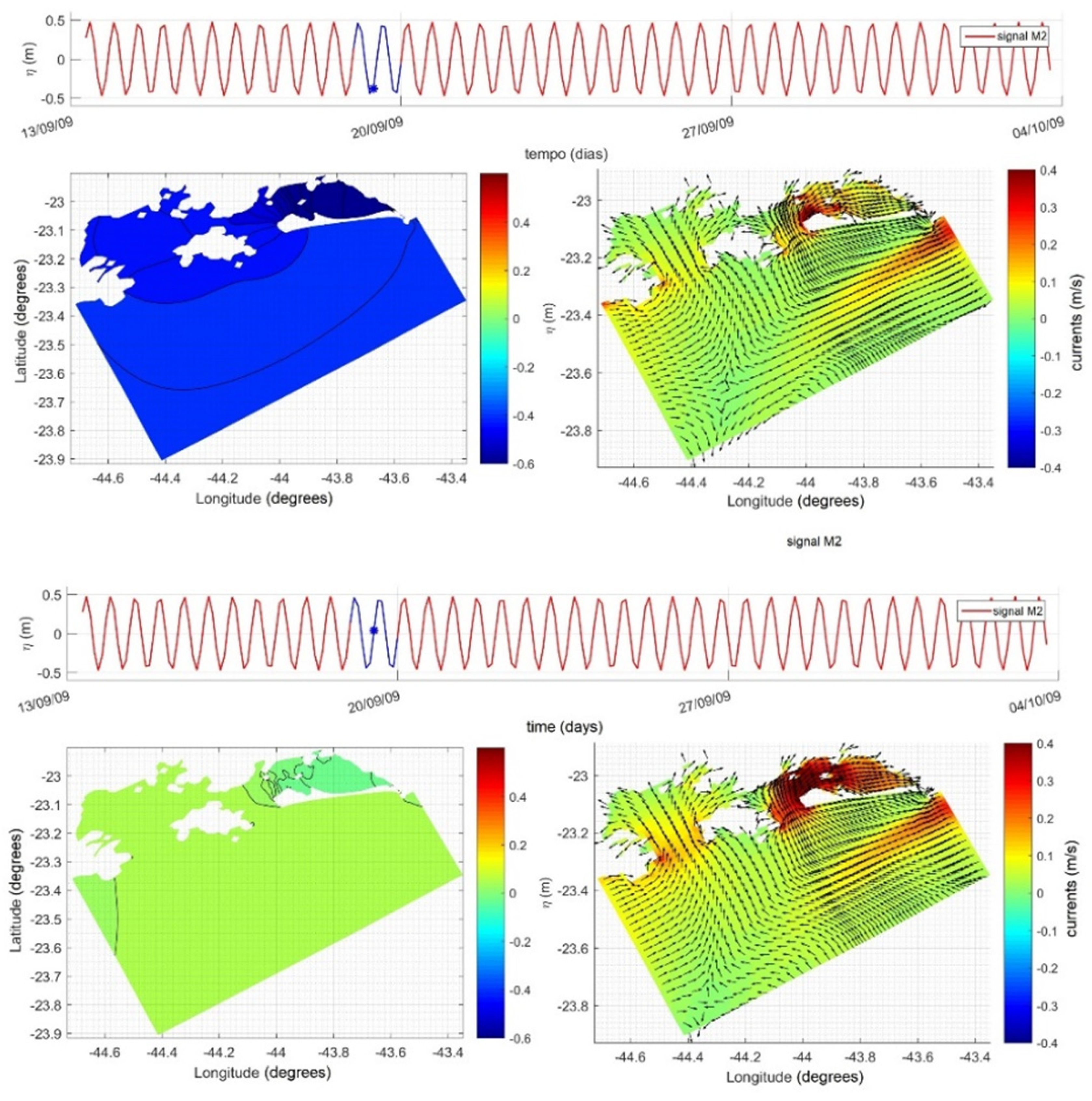
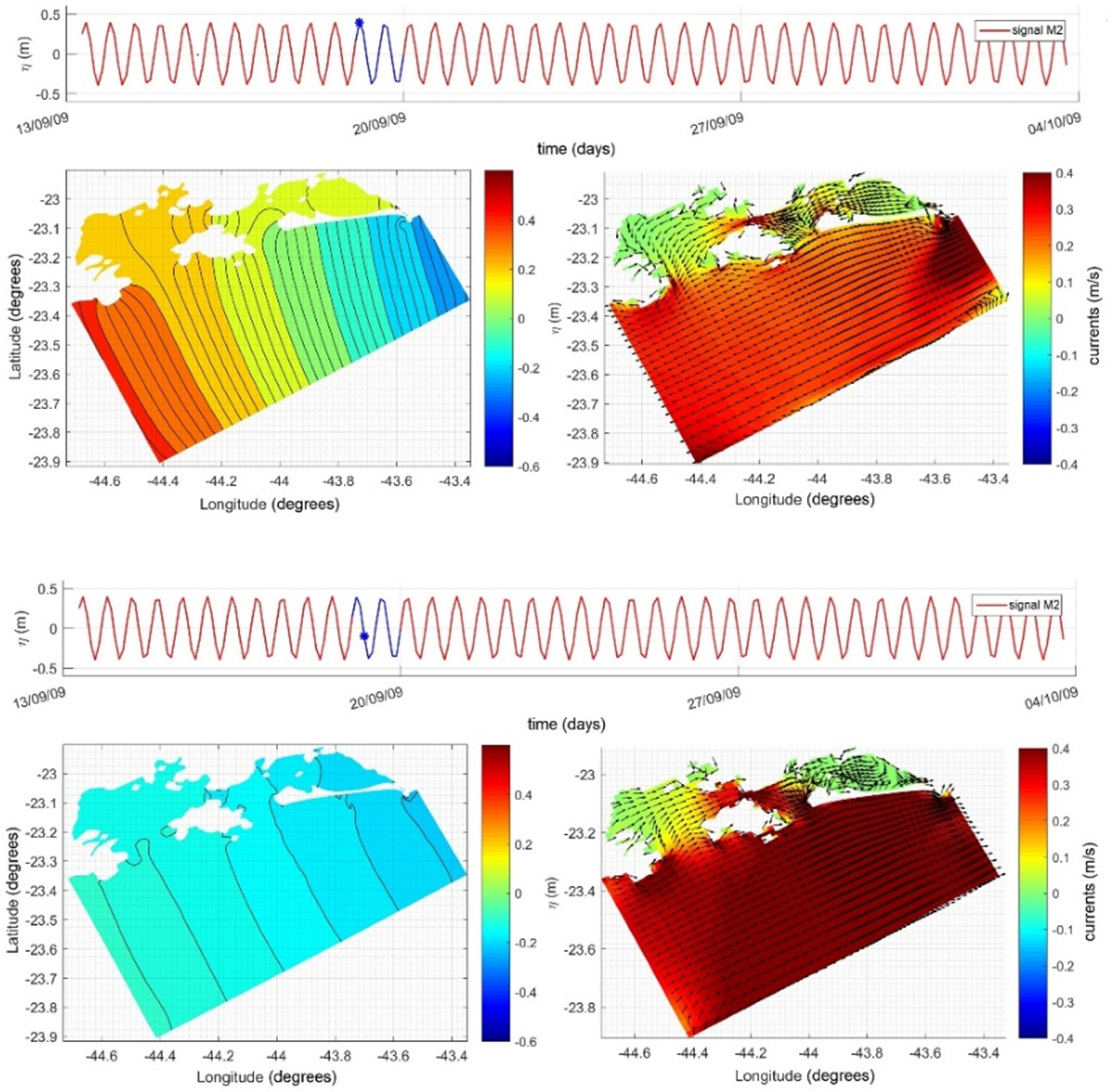
To gain a deeper understanding of the distinct behavior of astronomical and meteorological signals in our study area, we conducted an examination of the propagation of only the M2 component within the study area. This signal was introduced solely at the sea level, and we anticipated a response in the currents. We tested variations in the propagation direction and amplitude of this signal but found no significant alterations in the general patterns of the sea level and currents distribution. The relatively small difference in sea level between the eastern and western boundaries contributes to the more stationary nature of the astronomical signal. To further explore this, we conducted experiments introducing a lag of 1 min (S3 scenario), akin to the observed environmental conditions (as seen in Figure 20), and a lag of 4.92 h (S4 scenario), mirroring the meteorological signal (as seen in Figure 21).
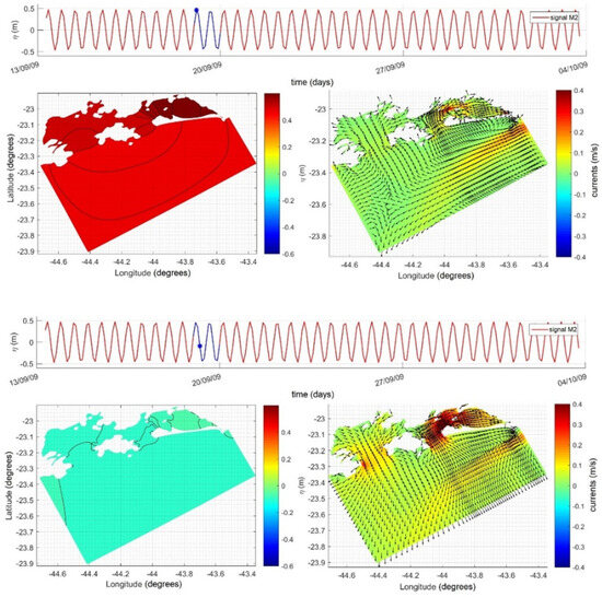
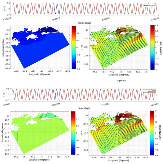
Figure 20.
Spatial variation in sea levels (on the left) and currents (on the right) in the Delft3D results for simulation considering only the M2 component with a lag of 1 min between the western and eastern borders for the following times from 19 September 2009 (from top to bottom): 2 h; 6 h; 10 h; 12 h. The instant represented by the spatial distribution is presented with a blue point in the time series of the artificial wave inserted at the model’s boundary, at the top of the images.

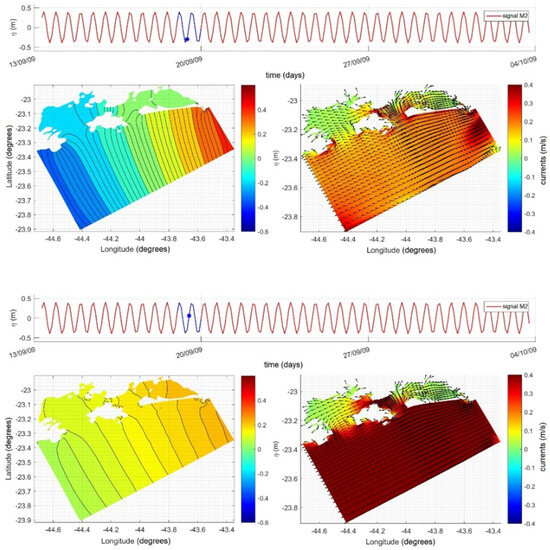
Figure 21.
Spatial variation in sea levels (on the left) and currents (on the right) in the Delft3D results for simulation considering only the M2 component with a lag of 4.92 h between the southern and northern borders for the following times from 19 September 2009 (from top to bottom): 2 h; 6 h; 10 h; 12 h. The instant represented by the spatial distribution is presented with a blue point in the time series of the artificial wave inserted at the model’s boundary, at the top of the images.
While an M2 tidal lag of just 1 min exhibited behavior closely reflecting the overall astronomical signal, the 4.92 h lag demonstrated characteristics remarkably akin to those of the meteorological signal. Only minor alterations in the current patterns were observed, which can be attributed to the introduction of boundary levels. Notably, the M2 currents associated with the 4.92 h lag were more robust than the original meteorological signal, likely due to the greater amplitude imposed on this signal. Directional changes were also evident, as M2 propagated southward, contrary to the meteorological signal, as discussed by Harari and Camargo [39].
From these experiments, we can infer that the stationary behavior of the astronomical signal is a direct consequence of its minimal lag at the external boundary. This short lag results in a small level gradient between the lateral boundaries compared to the gradient between the boundary parallel to the coast and the coastline. Consequently, at the bay entrances, the flow perpendicular to the coast results in the characteristic flood and ebb flows. As the signal enters Sepetiba Bay, due to the level gradient between the entrance and the innermost portion of the bay at the Bacalhau channel, the wave signal goes to transition into a progressive state with expressive tidal currents in this bay.
Increasing the lag of the wave signal leads to a greater level gradient between the lateral boundaries, favoring a flow parallel to the coast, as observed in the meteorological signal. While this flow exhibits higher intensity outside the bays, a portion of it finds its way into the bay entrances, bypassing Ilha Grande and passing through the channel between the island and the mainland, which intensifies currents in this region.
4. Conclusions
The water level observations from our model, incorporating both astronomical and meteorological signals, at a point within Sepetiba Bay exhibited a standard deviation of ±0.32 m. However, upon the removal of the astronomical signal, the same data still showed a standard deviation of ±0.08 m. This indicates that in Sepetiba Bay, while more affected by tides within the entire system, the meteorological signal still accounts for 25% of the total variance. Thus, it becomes evident that meteorological forcing cannot be disregarded in this system.
Comparing the meteorological forcing represented by the ocean model to available data reveals that the main features align well with the observed conditions in the area. Notably, the propagation speed exhibits northward movement in phase with the sea level, characteristic of coastal trapped waves. While this pattern aligns with literature reports, there is an observed underestimation of the signal’s intensity, which has also been reported previously. Furthermore, the coastal model highlights a further attenuation of the meteorological signal’s intensity near the coastline.
The coupling of the coastal model (Delft3D) with the ocean model (the HYCOM) using Riemann’s invariants proves effective in driving the coastal model with the meteorological sea level signal. This approach accounts for the velocity component normal to the boundary, and the coastal model aptly captures the flows along both the west and east boundaries, which are perpendicular to the along-shelf flow. The south boundary, parallel to the bathymetry, exhibits more intense tidal flow, yet the coastal model accurately simulates the boundary flows in all cases, particularly when assessing flow rates entering and exiting the boundaries. Thus, the ocean model adeptly captures the meteorological forcing on the continental shelf and transfers it into the coastal domain’s interior. This coastal model is tailored to address the intricacies of coastal geometry that are often overlooked in larger-scale models.
Focusing on the patterns of the tidal and non-tidal signals, a notable phase lag is observed in the meteorological signal in the open sea and the channel between Guaíba Island and the mainland. This phase lag is more pronounced in the meteorological component (near 5 h) compared to the astronomical component (almost 1 min). The gradient level field resulting from this time lag will be responsible for defining the current intensification pattern to be presented.
The short lag of the astronomical signal results in a small gradient level between the lateral boundaries compared to the gradient between the boundary parallel to the coast and the coastline. Consequently, the flow perpendicular to the coast results in the characteristic flood and ebb flows to the innermost portion of the bays.
On the other hand, the large lag of the meteorological signal leads to a greater gradient level between the lateral boundaries, favoring the parallel flow to the coast. This flow exhibits higher intensity outside the bays, but a portion of it finds its way into the bay entrances, intensifying the currents in the Ilha Grande Channel.
The results of these simulations of wave signals show the leading role of barotropic circulation in generating the current pattern observed in the region. We see that the sum of the different wave signals, with their different amplitudes and phase characteristics, can effectively reproduce the local circulation.
An examination of simulations with and without the meteorological signal underscores the significance of including the meteorological signal, as it significantly impacts the currents. The sea level and current intensities in the simulations considering the meteorological signal align well with the existing literature, accurately representing ebb and flow patterns. Conversely, excluding this signal results in an underestimation of intensities, particularly in the open sea, the channel between Guaíba Island and the mainland, and a substantial portion of Ilha Grande Bay.
In conclusion, the distinct hydrodynamic patterns associated with astronomical and meteorological signals are a reflection of their propagation characteristics on the continental shelf. The meteorological signal generates a level gradient parallel to the coast, intensifying currents in that direction. The differential level gradient between the main entrances of the bays results in a flow around Ilha Grande, playing a pivotal role in intensifying currents in the channel between the island and the mainland, exacerbated by the channel’s narrow geometry. On the other hand, the astronomical signal displays a high-level gradient onshore, driving more robust ebb and flow currents at the bays’ entrances. The channel between Ilha Grande and the mainland serves as a point of convergence/divergence for this flow, with very low current velocities. Further investigations into the baroclinic influences and nonlinear interactions of sea level signals on circulation in the inner portions of the bays are recommended for a further understanding of their roles in the circulation dynamics.
Author Contributions
Conceptualization, N.E.d.S.P. and S.B.V.; methodology, N.E.d.S.P.; software, N.E.d.S.P.; validation, N.E.d.S.P.; formal analysis, N.E.d.S.P.; investigation, N.E.d.S.P.; resources, N.E.d.S.P. and S.B.V.; data curation, N.E.d.S.P.; writing—original draft preparation, N.E.d.S.P.; writing—review and editing, N.E.d.S.P., S.B.V., M.N.G. and M.G.; visualization, N.E.d.S.P.; supervision, S.B.V.; project administration, S.B.V.; funding acquisition, S.B.V. All authors have read and agreed to the published version of the manuscript.
Funding
The first author was financially supported by CAPES (Coordenação de Aperfeiçoamento de Pessoal de Nível Superior—Brazil)—Finance Code 001. The second and third authors were also financially supported by CNPq (Conselho Nacional de Desenvolvimento Científico e Tecnológico) through Grants 310132/2019-3 and 309055/2022-9.
Data Availability Statement
The data used in this work are available on request to the corresponding author.
Acknowledgments
We also acknowledge the support of our colleagues and everyone who contributed to this project.
Conflicts of Interest
The authors declare no conflicts of interest.
References
- Nicholls, R.J.; Kebede, A.S. Indirect impacts of coastal climate change and sea-level rise: The UK example. Clim. Policy 2012, 12 (Suppl. S1), S28–S52. [Google Scholar] [CrossRef]
- Andrade, M.M.; Toldo, E.E.; Nunes, J.C.R. Tidal and subtidal oscillations in a shallow water system in southern Brazil. Braz. J. Oceanogr. 2018, 66, 245–254. [Google Scholar] [CrossRef]
- Mestres, M.; Grifoll, M.; Sánchez-Arcilla, A. Analysis of current intensification in the Northwest Mediterranean shelf. Cont. Shelf Res. 2016, 114, 29–40. [Google Scholar] [CrossRef]
- WMO. Atlas of Mortality and Economic Losses from Weather, Climate, and Water Extremes (1970–2019); World Meteorological Organization (WMO): Geneva, Switzerland, 2021; p. 90. [Google Scholar]
- Pugh, D. Tides, Surges, and Mean Sea-Level; John Wiley & Sons: New York, NY, USA, 1987; p. 486. [Google Scholar]
- Bowden, K.F. Physical Oceanography of Coastal Waters; Ellis Horwood Ser. Mar. Sci. John Wiley & Sons, Inc.: Sometset, NJ, USA, 1983; p. 302. [Google Scholar] [CrossRef]
- Open University. Waves, Tides and Shallow-Water Processes, 2nd ed.; Butterworth-Heinemann: Oxford, UK, 1999; p. 227. [Google Scholar]
- Marone, E.; Camargo, R. Marés meteorológicas no litoral do estado do Paraná: O evento de 18 de Agosto de 1993. Nerítica 1994, 8, 73–85. [Google Scholar]
- Wang, B. Kelvin Waves. In Encyclopedia of Atmospheric Sciences; Shankar, M., Ed.; Elsevier Science Ltd.: Amsterdam, Netherlands, 2002; p. 7. [Google Scholar]
- Wang, D.P.; Mooers, C.N.K. Coastal-trapped waves in a continuous stratified ocean. J. Phys. Oceanogr. 1976, 6, 853–863. [Google Scholar] [CrossRef]
- Platov, G.A. The influence of shelf zone topography and coastline geometry on coastal trapped waves. Numer. Anal. Appl. 2016, 9, 231–245. [Google Scholar] [CrossRef]
- Mysak, L.A. Topographically trapped waves. Annu. Rev. Fluid Mech. 1980, 12, 45–76. [Google Scholar] [CrossRef]
- Idier, D.; Bertin, X.; Thompson, P.; Pickering, M.D. Interactions Between Mean Sea Level, Tide, Surge, Waves and Flooding: Mechanisms and Contributions to Sea Level Variations at the Coast. Surv. Geophys. 2019, 40, 1603–1630. [Google Scholar] [CrossRef]
- Wang, D.P.; Elliott, A.J. Non-Tidal Variability in the Chesapeake Bey and Potomac River: Evidence for Non-Local Forcing. J. Phys. Oceanogr. 1978, 8, 225–232. [Google Scholar] [CrossRef]
- Garvine, R.W. A simple model of estuarine subtidal fluctuations forced by local and remote wind stress. J. Geophys. Res. 1985, 90, 11945–11948. [Google Scholar] [CrossRef]
- Zhong, L.; Li, M.; Zhang, D.-L. How do uncertainties in hurricane model forecasts affect storm surge predictions in a semi-enclosed bay? Estuar. Coast. Shelf Sci. 2010, 90, 61–72. [Google Scholar] [CrossRef]
- Melo Filho, E. Maré Meteorológica na Costa Brasileira. Associate Professorship Thesis, Universidade Federal de Rio Grande, Rio Grande, Brazil, 2017. Available online: https://www.researchgate.net/profile/Eloi-Melo/publication/318710781_Mare_Meteorologica_na_Costa_Brasileira/links/5979090f0f7e9b27772a250a/Mare-Meteorologica-na-Costa-Brasileira.pdf (accessed on 20 November 2023).
- Truccolo, E.C.; Franco, D.; Schettini, C.A.F. The low frequency sea level oscillations in the northern coast of Santa Catarina, Brazil. J. Coast. Res. 2006, SI 39, 547–552. [Google Scholar]
- Oliveira, M.M.F.; Ebecken, N.F.F.; Santos, I.A.; Neves, C.F.; Caloba, L.P.; Oliveira, J.L.F.M. Modelagem da maré meteorológica utilizando redes neurais artificiais: Uma aplicação para a Baía de Paranaguá—PR, Parte 1: Dados meteorológicos da estação de superfície. Rev. Bras. Meteorol. 2006, 21, 220–231. [Google Scholar]
- Verlaan, M.; Zijderveld, A.; de Vries, H.; Kroos, J. Operational storm surge forecasting in the Netherlands: Developments in the last decade. Philos. Trans. R. Soc. A Math. Phys. Eng. Sci. 2005, 363, 1441–1453. [Google Scholar] [CrossRef]
- Cavalcante, S.L.S.; Rosman, P.C.C.A. Circulação e transporte no Complexo da Baía de Ilha Grande e Sepetiba via aninhamento de modelo numérico—Período de inverno. Anais Hidrográficos 2010, 67, 117–126. [Google Scholar]
- Fiedler, M.; Siegle, E. Estuarine Dynamics in Climate Change Scenarios: Santos Estuary, SP. In Proceedings of the 17th PECS, Porto de Galinhas, Brazil, 19–23 October 2014. [Google Scholar]
- Veleda, D.; Araujo, M.; Zantopp, R.; Montagne, R. Intraseasonal variability of the North Brazil Undercurrent forced by remote winds. J. Geophys. Res. Ocean. 2012, 117, 1–10. [Google Scholar] [CrossRef]
- Brink, K.H. Propagation of Barotropic Continental Shelf Waves over Irregular Bottom Topography. J. Phys. Oceanogr. 1980, 10, 765–778. [Google Scholar] [CrossRef]
- Freitas, P.P.; Paiva, A.M.; Cirano, M.; Mill, G.N.; Costa, V.S.; Gabioux, M.; França, B.R.L. Coastal trapped waves propagation along the Southwestern Atlantic Continental Shelf. Cont. Shelf Res. 2021, 226, 104496. [Google Scholar] [CrossRef]
- Sandstrom, H. On the Wind-Induced Sea Level Changes on the Scotian Shelf. J. Geophys. Res. 1980, 85, 461–468. [Google Scholar] [CrossRef]
- Fiedler, M.F.M. Dinâmica Estuarina em Cenário de Aumento do Nível do Mar: Estuário de Santos, SP. Master’s Thesis, Universidade de São Paulo, São Paulo, Brazil, 2015. Available online: https://teses.usp.br/teses/disponiveis/21/21136/tde-26022016-144937/publico/Dissertacao_Fiedler_MariaFernanda_Corrigida.pdf (accessed on 24 November 2023).
- Castro, B.M.; Lee, T.N. Wind-forced sea level variability on the southeast Brazilian shelf. J. Geophys. Res. 1995, 100, 16045–16056. [Google Scholar] [CrossRef]
- França, B.R.L. Ondas Confinadas Costeiras na Plataforma Continental Sul-sudeste do Brasil. Master’s Thesis, Universidade Federal do Rio de Janeiro, Rio de Janeiro, Brazil, 2013. Available online: https://w1files.solucaoatrio.net.br/atrio/ufrj-peno_upl/THESIS/6000264/2013_mestrando_bruna_reis_leite_franca_20200405213423662.pdf (accessed on 27 November 2023).
- Dottori, M.; Castro, B.M. The role of remote wind forcing in the subinertial current variability in the central and northern parts of the South Brazil Bight. Ocean Dyn. 2018, 68, 677–688. [Google Scholar] [CrossRef]
- Rodrigues, D.; Fernandes, A.; Filippo, A.; Kjerfve, B.; Pinto, L.; Neves, R. Low-frequency circulation on the Ilha Grande channel, Rio de Janeiro, Brazil. Reg. Stud. Mar. Sci. 2022, 50, 102129. [Google Scholar] [CrossRef]
- Miranda, L.B.; Ikeda, Y.; Castro Filho, B.M.; Pereira Filho, N. Note on the occurrence of saline fronts in the Ilha Grande (RJ) region. Boletim do Instituto Oceanográfico 1977, 26, 249–256. [Google Scholar] [CrossRef]
- Signorini, S.R. A study of the circulation in Bay of Ilha Grande and Bay of Sepetiba: Part I. a survey of the circulation based on experimental field data. Boletim do Instituto Oceanográfico 1980, 29, 41–55. [Google Scholar] [CrossRef]
- Signorini, S.R. A study of the circulation in Bay of Ilha Grande and Bay of Sepetiba: Part II: An assessment to the tidally and wind-driven circulation using a finite element numerical model. Boletim do Instituto Oceanográfico 1980, 29, 57–68. [Google Scholar] [CrossRef]
- Kjerfve, B.; Dias, G.T.M.; Filippo, A.; Geraldes, M.C. Oceanographic and environmental characteristics of a coupled coastal bay system: Baía de Ilha Grande-Baía de Sepetiba, Rio de Janeiro, Brazil. Reg. Stud. Mar. Sci. 2021, 41, 101594. [Google Scholar] [CrossRef]
- Fragoso, M.R. Estudo Numérico da Circulação Marinha da Região das Baías de Sepetiba e Ilha Grande (RJ). Master’s Thesis, Universidade de São Paulo, São Paulo, Brazil, 1999. [Google Scholar]
- Cavalcante, S.L.S. Estudo da Influência da Dinâmica da Plataforma Continental nas Baías de Ilha Grande e Sepetiba Via Aninhamento de Modelo Numérico Costeiro a Modelo Numérico Oceânico. Ph.D. Thesis, Universidade Federal do Rio de Janeiro, Rio de Janeiro, Brazil, 2010. Available online: https://biblioteca.sdm.mar.mil.br/bitstream/ripcmb/844610/1/Tese%20CMG%20Sonia.pdf (accessed on 15 November 2023).
- Barros, C.P.; Felício, J.A.; Fernandes, R.L. Productivity analysis of Brazilian seaports. Marit. Policy Manag. 2012, 39, 503–523. [Google Scholar] [CrossRef]
- Harari, J.; Camargo, R. Simulação da propagação das nove principais componentes de maré na plataforma sudeste brasileira através de modelo numérico hidrodinâmico. Boletim do Instituto Oceanográfico 1994, 42, 35–54. [Google Scholar] [CrossRef]
- Chassignet, E.P.; Hurlburt, H.E.; Smedstad, O.M.; Halliwell, G.R.; Hogan, P.J.; Wallcraft, A.J.; Baraille, R.; Bleck, R. The HYCOM (HYbrid Coordinate Ocean Model) data assimilative system. J. Mar. Syst. 2007, 65, 60–83. [Google Scholar] [CrossRef]
- Bleck, R. An oceanic general circulation model framed in hybrid isopycnic-Cartesian coordinates. Ocean Model. 2002, 4, 55–88. [Google Scholar] [CrossRef]
- Deltares. Delft3D-FLOW Simulation of Multi-Dimensional Hydrodynamic Flows and Transport Phenomena, Including Sediments: User Manual, Version 3.04; Deltares: Delft, The Netherlands, 2014.
- Ye, Q.; Morelissen, R.; Goede, E.D.; Ormondt, M.V.; Kester, J.V. A new technique for nested boundary conditions in hydrodynamic modeling. Asian Pac. Coasts 2011, 1368–1377. [Google Scholar] [CrossRef]
- Gabioux, M.G.; Da Costa, V.S.; de Souza, J.M.A.C.; de Oliveira, B.F.; Paiva, A.M. Modeling the South Atlantic Ocean from medium to high-resolution. Revista Brasileira de Geofísica 2013, 31, 229–242. [Google Scholar] [CrossRef]
- Costa, V.S.; Mill, G.N.; Gabioux, M.; Grossmann-Matheson, G.S.; Paiva, A.M. The recirculation of the intermediate western boundary current at the Tubarão Bight–Brazil. Deep-Sea Res. Part I Oceanogr. Res. Pap. 2017, 120, 48–60. [Google Scholar] [CrossRef]
- Lima, J.A.M.; Martins, R.P.; Tanajura, C.A.S.; Paiva, A.M.; Cirano, M.; Campos, E.J.D.; Soares, I.D.; França, G.B.; Obino, R.S.; Alvarenga, J.B.R. Design and implementation of the Oceanographic modeling and observation Network (REMO) for operational oceanography and ocean forecasting. Revista Brasileira de Geofísica 2013, 31, 209–228. [Google Scholar] [CrossRef]
- Egbert, G.D.; Erofeeva, S.Y. Efficient inverse modeling of barotropic ocean tides. J. Atmos. Ocean. Technol. 2002, 19, 183–204. [Google Scholar] [CrossRef]
- Ponçano, W.L. Sedimentação Atual na Baía de Sepetiba, Estado do Rio de Janeiro. Master’s Thesis, Universidade de São Paulo, São Paulo, Brazil, 1976. Available online: https://www.teses.usp.br/teses/disponiveis/44/44131/tde-14102015-150048/pt-br.php (accessed on 19 November 2023).
- Mahiques, M.M. Considerações Sobre os Sedimentos de Superfície de Fundo da Baía de Ilha Grande, Estado do Rio de Janeiro. Master’s Thesis, Universidade de São Paulo, São Paulo, Brazil, 1987. Available online: https://teses.usp.br/teses/disponiveis/21/21132/tde-13102009-164145/publico/Mahiques.pdf (accessed on 24 November 2023).
- Nikuradse, J. Laws of Flow in Rough Pipes; Translation of “Stromungsgesetze in rauhen Rohren.” VDI-Forschungsheft 361. Beilage zu “Forschung auf dem Gebiete des Ingenieurwesens” Ausgabe B Band 4, 1933; NACA: Washington, DC, USA, 1950. [Google Scholar]
- Diederen, D.; Savenije, H.H.G.; Toffolon, M. The open boundary equation. Ocean Sci. Discuss. 2015, 12, 925–958. [Google Scholar] [CrossRef]
- Verboom, G.K.; Slob, A. Weakly-reflective boundary conditions for two-dimensional shallow water flow problems. Adv. Water Resour. 1984, 7, 192–197. [Google Scholar] [CrossRef]
- Van Wageningen-Kessels, F. Convergence of QuickFlow: A Steady State Solver for the Shallow Water Equations; Report Literature Study; Delft University of Technology: Delft, The Netherlands, 2006. [Google Scholar]
- Fonseca, S.A.R. Circulação e Fluxo de Material Particulado em Suspensão no Principal Canal de Acesso à Baía de Sepetiba. Master’s Thesis, Universidade Estadual do Rio de Janeiro, Rio de Janeiro, Brazil, 2013. Available online: https://www.bdtd.uerj.br:8443/handle/1/13884 (accessed on 27 November 2023).
- Cerqueira, E.O.; Poppi, R.J.; Kubota, L.T. Utilização de filtro de Transfomada de Fourier para a minimização de ruídos em sinais analíticos. Química Nova 2000, 23, 690–698. [Google Scholar] [CrossRef]
- Carvalho, R.A. Estudo da variabilidade do nível médio do mar na costa brasileira como subsídio a projetos de engenharia. Master’s Thesis, Universidade Federal do Rio de Janeiro, Rio de Janeiro, Brazil, 2015. Available online: http://www.repositorio.poli.ufrj.br/monografias/monopoli10015355.pdf (accessed on 28 November 2023).
- Pawlowicz, R.; Beardsley, B.; Lentz, S. Classical tidal harmonic analysis including error estimates in MATLAB using T_TIDE. Comput. Geosci. 2002, 28, 929–937. [Google Scholar] [CrossRef]
- IOC. Global Sea Level Observing System (GLOSS) Implementation Plan—2012; Technical Series, 100; UNESCO/Intergovernmental Oceanographic Commission: Paris, France, 2012; p. 41. [Google Scholar]
- Box, G.E.P.; Jenkins, G.M.; Reinsel, G.C. Time Series Analysis: Forecasting and Control, 4th ed.; John Wiley & Sons: Hoboken, NJ, USA, 2008; p. 746. [Google Scholar]
- Willmott, C.J. On the validation of models. Phys. Geogr. 1981, 2, 184–194. [Google Scholar] [CrossRef]
- Chen, F.; Shapiro, G.; Thain, R. Sensitivity of Sea Surface Temperature Simulation by an Ocean Model to the Resolution of the Meteorological Forcing. ISRN Oceanogr. 2013, 2013, 215715. [Google Scholar] [CrossRef]
- Sutherland, J. COSMOS Modelling and the Development of Model Performance Statistics; TR121-EC MAST Project no MAS3-CT97-0086; HR Wallingford: Wallingford, UK, 2001; pp. B4.1–B4.4. [Google Scholar]
- Willmott, C.J. Some Comments on the Evaluation of Model Performance. Bull. Am. Meteorol. Soc. 1982, 63, 1309–1313. [Google Scholar] [CrossRef]
- Stech, J.L.; Lorenzzetti, J.A. The Response of the South Brazil Bight to Wintertime Cold Fronts. J. Geophys. Res. 1992, 97, 9507–9520. [Google Scholar] [CrossRef]
- Zamudio, L.; Hurlburt, H.E.; Metzger, E.J.; Smedstad, O.M. On the evolution of coastally trapped waves generated by Hurricane Juliette along the Mexican West Coast: Hurricane Juliette and Coastal Waves. Geophys. Res. Lett. 2002, 29, 56-1–56-4. [Google Scholar] [CrossRef]
- Teixeira, G.L.G.; Mazzuco, D.P.; Donin Júnior, D.J.; Santanada, F.R.; Tecchio, R.; Daher, V.B. Influência dos diferentes comprimentos de séries temporais na análise harmônica da maré astronômica na Baía de Sepetiba—Rio de Janeiro, Brasil. Anais Hidrográficos 2017, 73, 103–112. [Google Scholar]
- Pairaud, I.L.; Lyard, F.; Auclair, F.; Letellie, T.; Marsaleix, P. Dynamics of the semi-diurnal and quarter-diurnal internal tides in the Bay of Biscay. Part 1: Barotropic tides. Cont. Shelf Res. 2008, 28, 1294–1315. [Google Scholar] [CrossRef]
- Campos, R.M.; De Camargo, R.; Harari, J. Caracterização de eventos extremos do nível do mar em Santos e sua correspondência com as re-análises do modelo do NCEP no Sudoeste do Atlântico Sul. Revista Brasileira de Meteorologia 2010, 25, 2. [Google Scholar] [CrossRef]
- Gutiérrez, M.O.; López, M.; Candela, J.; Castro, R.; Mascarenhas, A.; Collins, C.A. Effect of coastal-trapped waves and wind on currents and transport in the Gulf of California. J. Geophys. Res. Ocean. 2014, 119, 5123–5139. [Google Scholar] [CrossRef]
- Wilkin, J.L.; Chapman, D.C. Scattering of Coastal-Trapped Waves by Irregularities in Coasline and Topography. J. Phys. Oceanogr. 1990, 20, 396–421. [Google Scholar] [CrossRef]
- Daher, V.B.; Nogueira, I.C.M.; Ribeiro, C.E.P.; Rosman, P.C.C. Análise das Estimativas de Maré Meteorológica pelo Modelo Oceânico Global HYCOM/NCODA na Região ao Largo da Baía da Ilha Grande—Rj. Anais Hidrográficos 2017, 73, 114–125. [Google Scholar]
- Mordente, T.Z. Estudo da Hidrodinâmica das Baías de Ilha Grande e Sepetiba. Master’s Thesis, Universidade Federal do Espírito Santo, Vitória, Brazil, 2020. Available online: https://sucupira.capes.gov.br/sucupira/public/consultas/coleta/trabalhoConclusao/viewTrabalhoConclusao.jsf?popup=true&id_trabalho=9478807 (accessed on 2 January 2023).
- Fonseca, S.A.R.; Guerra, J.V. Observações dos Padrões de Circulação nas Proximidades do Canal de Navegação da Baía De Sepetiba (RJ)—Agosto de 2011; Anais do X ENES: Foz do Iguaçu, PR, Brazil, 2012. [Google Scholar]
Disclaimer/Publisher’s Note: The statements, opinions and data contained in all publications are solely those of the individual author(s) and contributor(s) and not of MDPI and/or the editor(s). MDPI and/or the editor(s) disclaim responsibility for any injury to people or property resulting from any ideas, methods, instructions or products referred to in the content. |
© 2024 by the authors. Licensee MDPI, Basel, Switzerland. This article is an open access article distributed under the terms and conditions of the Creative Commons Attribution (CC BY) license (https://creativecommons.org/licenses/by/4.0/).


