
Channel Morphology Change after Restoration: Drone Laser Scanning versus Traditional Surveying Techniques


Abstract
1. Introduction
2. Materials and Methods
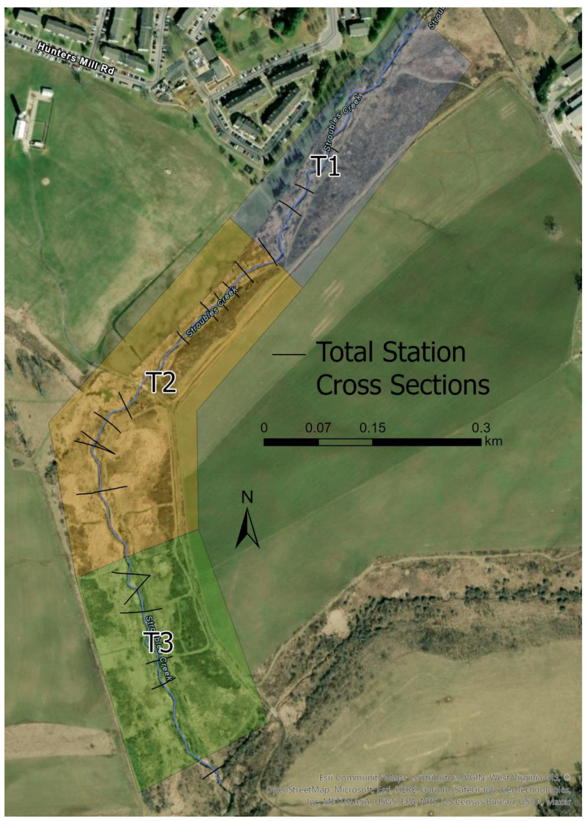
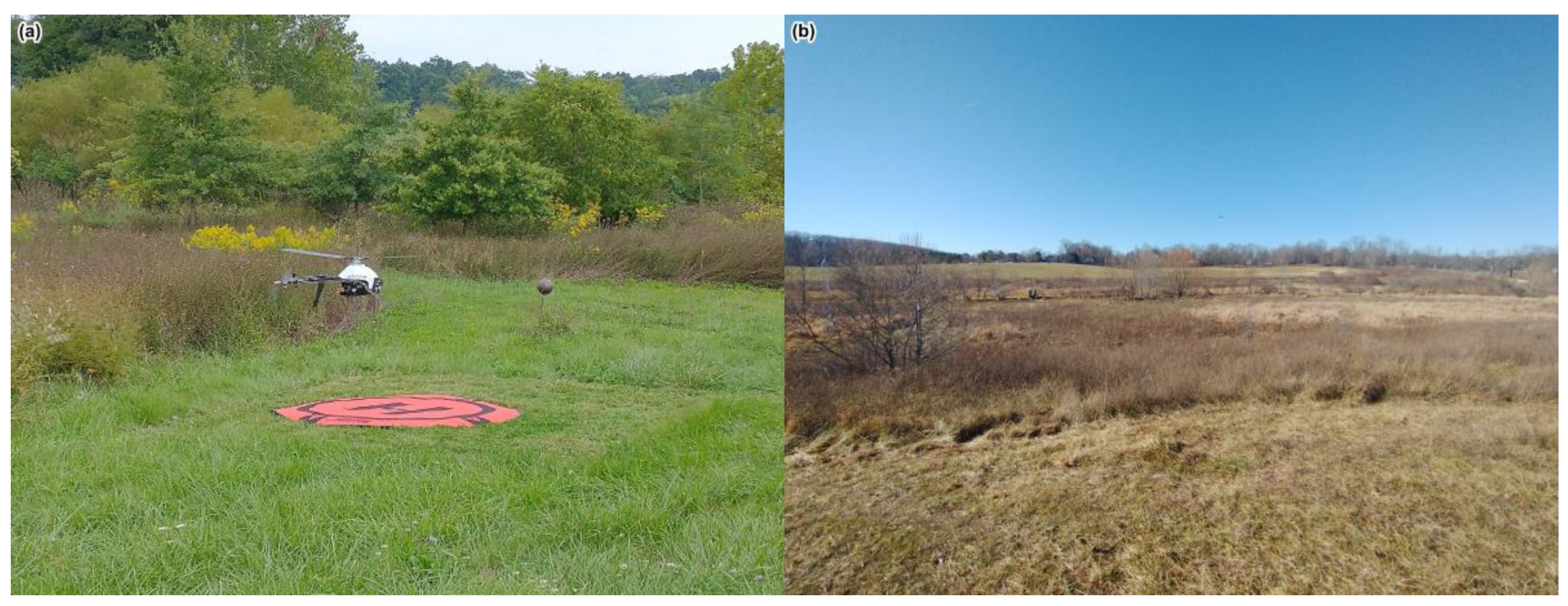
2.1. Study Area
2.2. Data Collection and Processing
2.2.1. Total Station Survey Data Collection
2.2.2. Drone Lidar Data Collection
2.2.3. Drone Lidar Data Processing
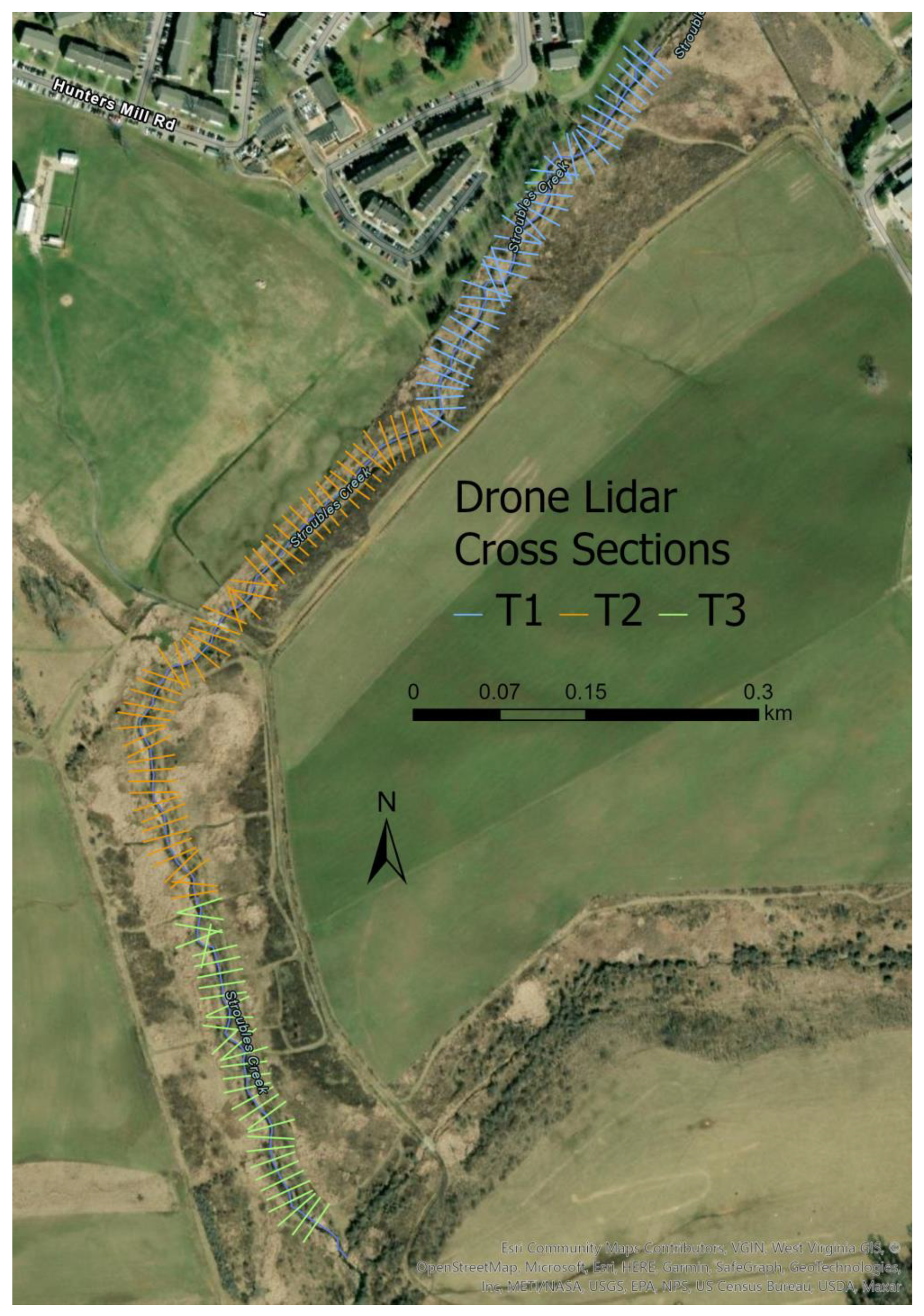
2.2.4. Generating Cross Sections from Drone Lidar Data
2.3. Deriving Channel Morphology Metrics
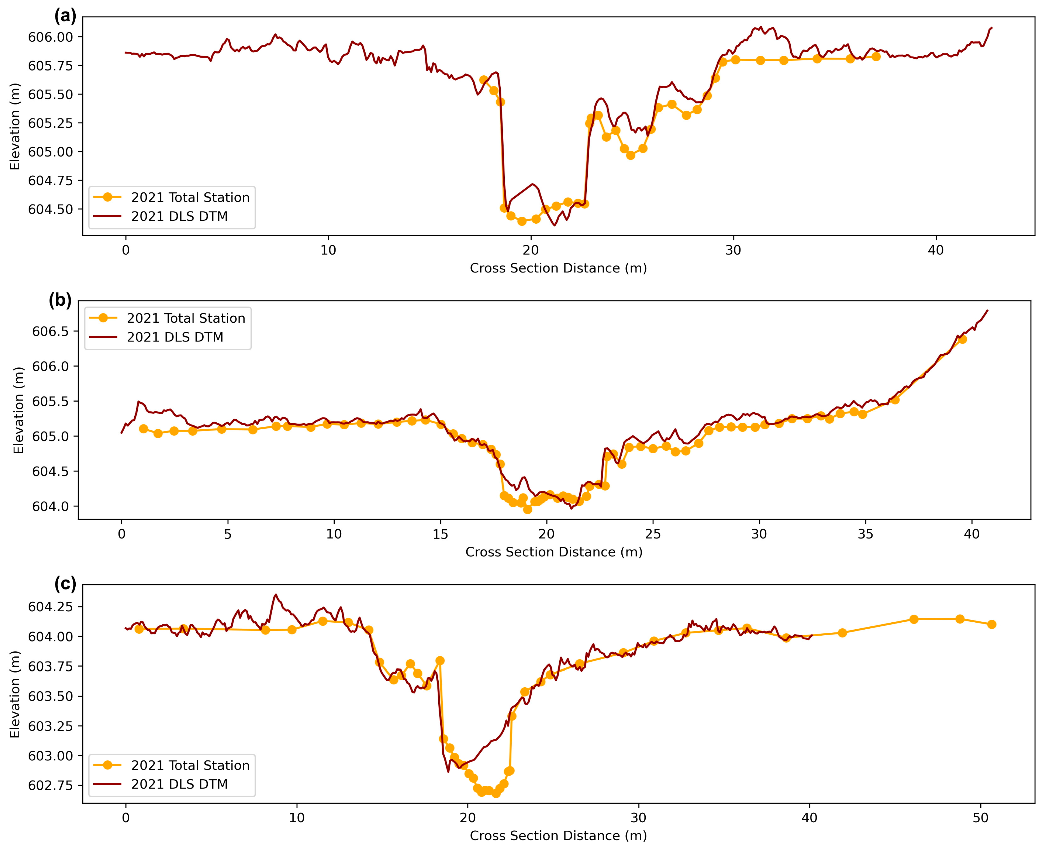
2.4. Comparing Cross-Sectional Metrics between Total Station and Drone Lidar Data
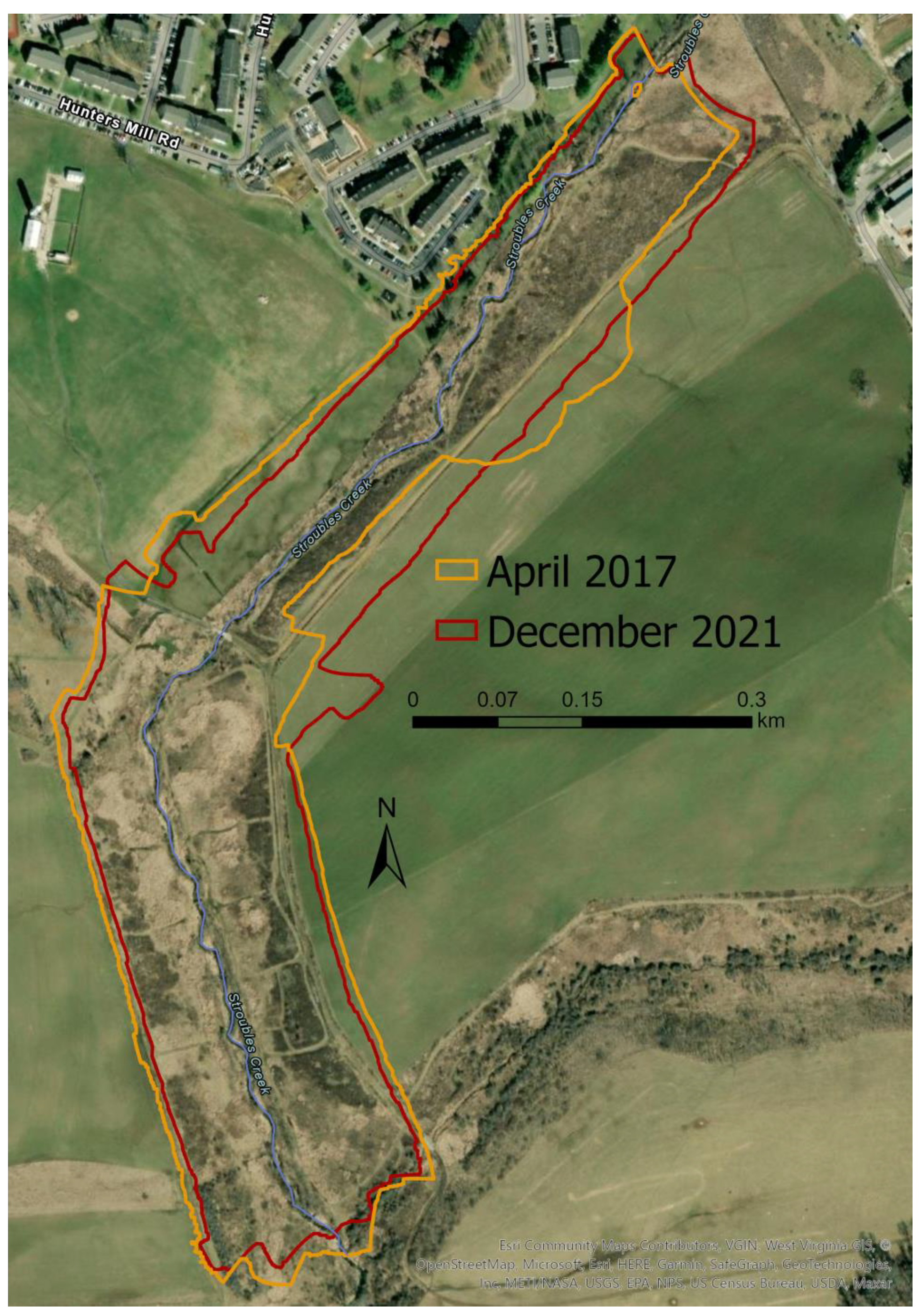
2.5. Quantifying Channel Morphology Changes between Restoration Treatments
3. Results and Discussion
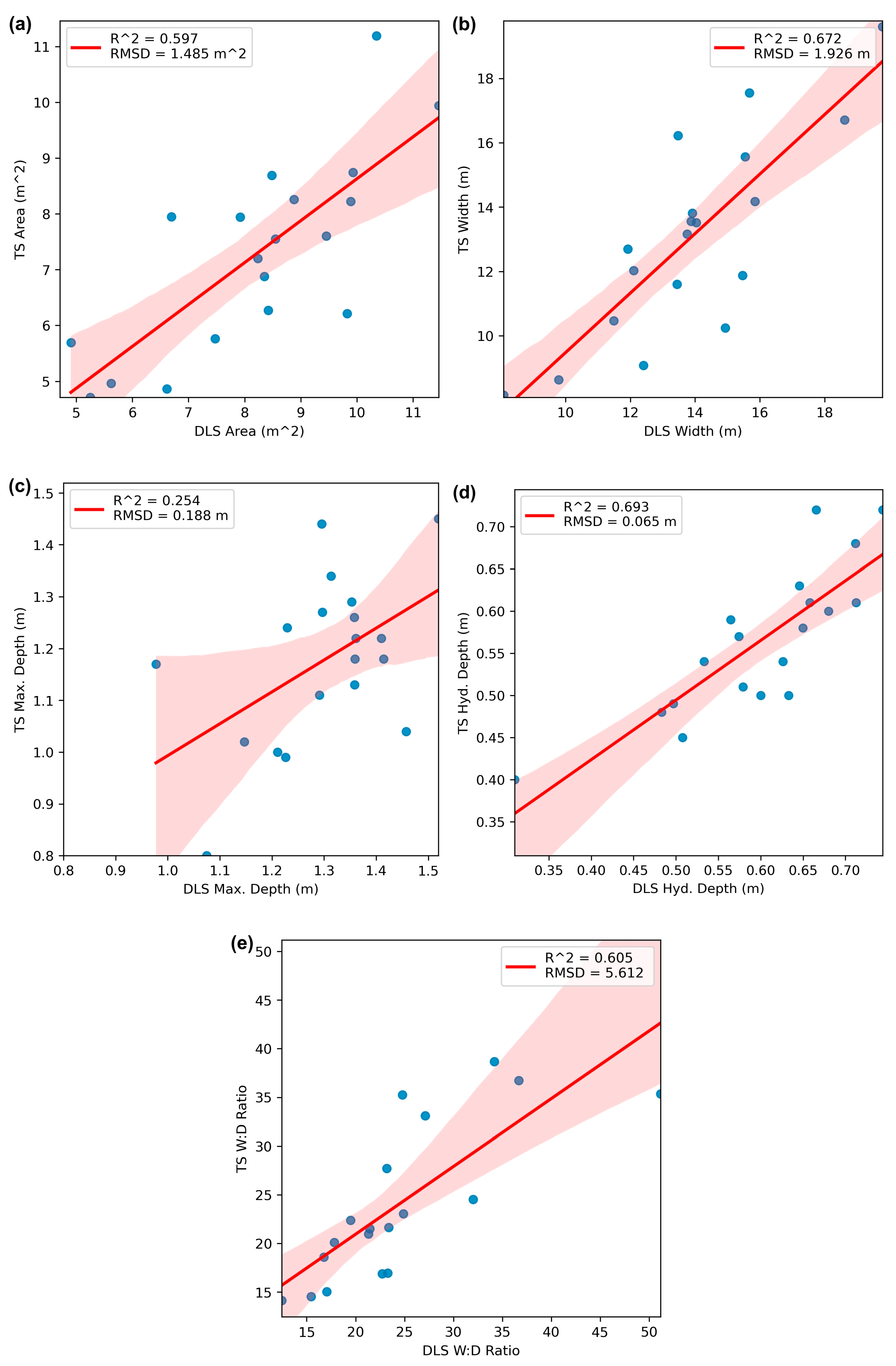
3.1. Comparing Cross-Sectional Metrics between Total Station and Drone Lidar Data
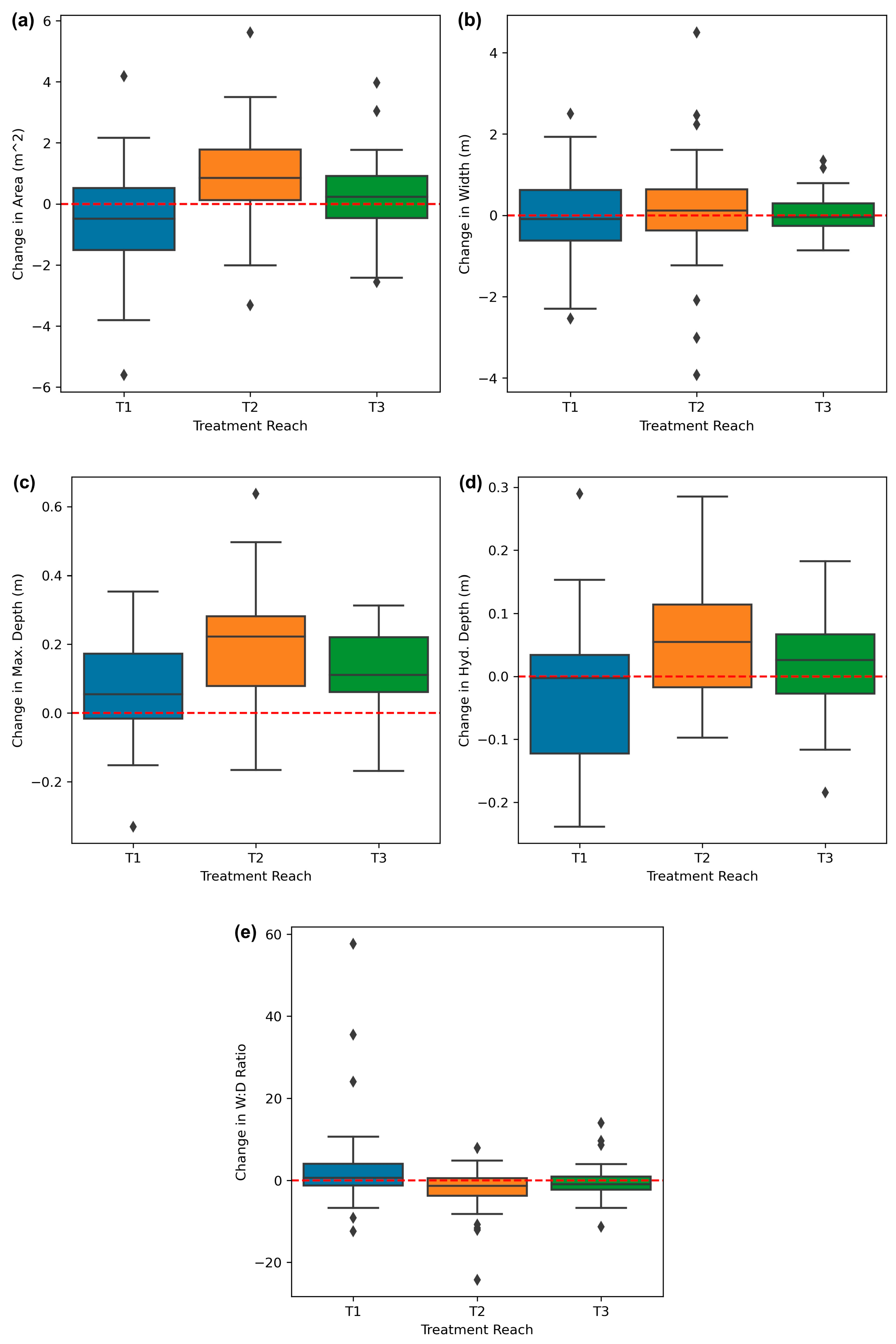
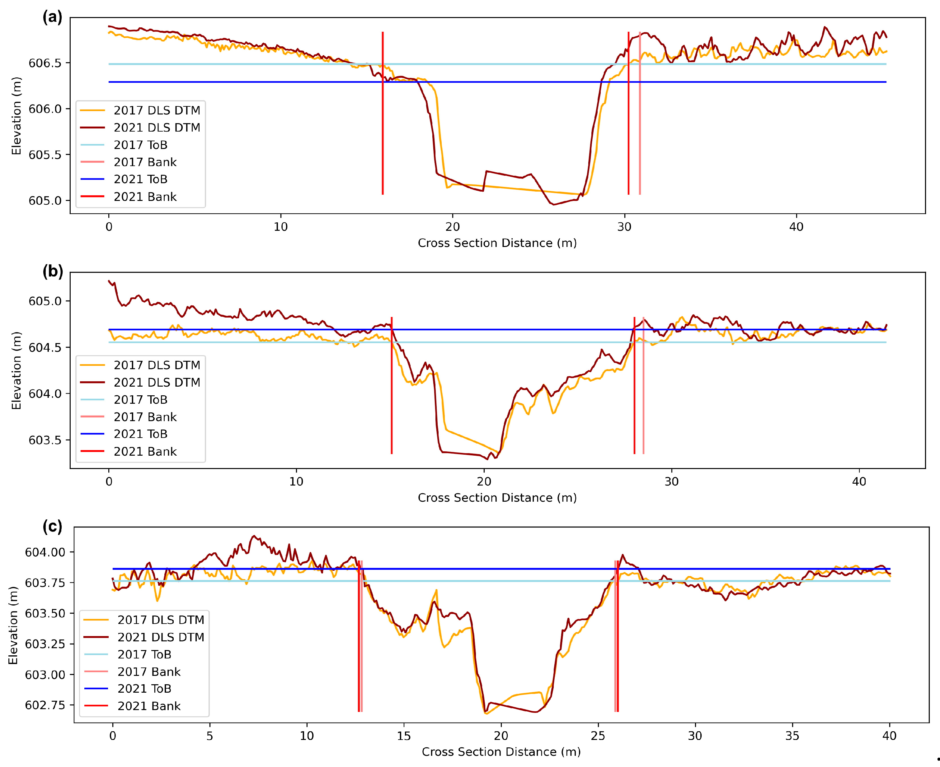
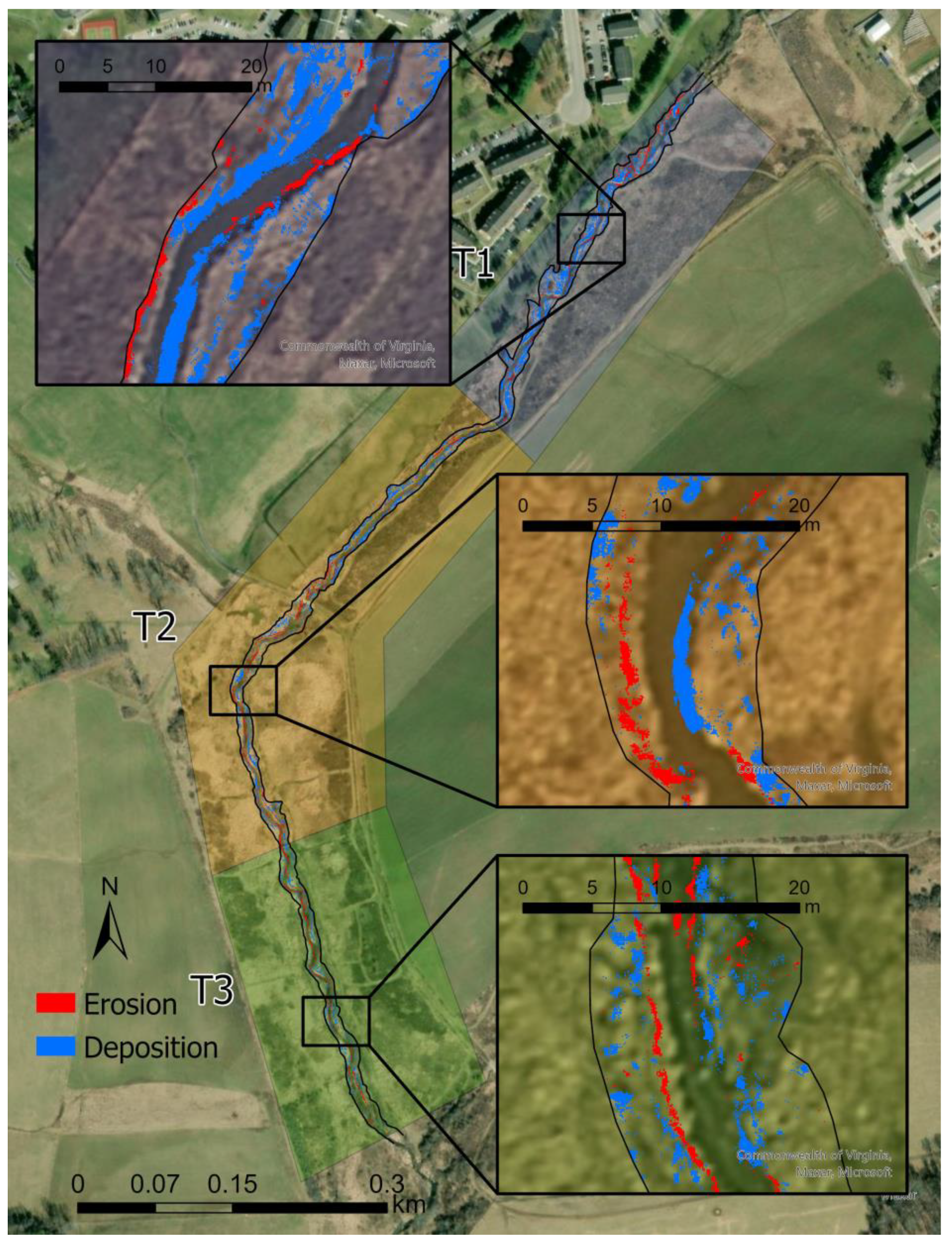
3.2. Quantifying Channel Morphology Changes between Restoration Treatments
4. Conclusions
Author Contributions
Funding
Data Availability Statement
Acknowledgments
Conflicts of Interest
References
- Bernhardt, E.S.; Palmer, M.A.; Allan, J.D.; Alexander, G.; Barnas, K.; Brooks, S.; Carr, J.; Clayton, S.; Dahm, C.; Follstad-Shah, J.; et al. Synthesizing U.S. River Restoration Efforts. Science 2005, 308, 636–637. [Google Scholar] [CrossRef]
- Wheeler, T.B. Stream Restoration Techniques Draw Pushback. Available online: https://www.bayjournal.com/news/pollution/stream-restoration-techniques-draw-pushback/article_ffc96960-0895-11eb-b36f-efa466158524.html (accessed on 11 June 2023).
- Shields, F.D.; Copeland, R.R.; Klingeman, P.C.; Doyle, M.W.; Simon, A. Design for Stream Restoration. J. Hydraul. Eng. 2003, 129, 575–584. [Google Scholar] [CrossRef]
- Doll, B.A.; Grabow, G.L.; Hall, K.R.; Halley, J.; Harman, W.A.; Jennings, G.D.; Wise, D.E. Stream Restoration: A Natural Channel Design Handbook; NC Stream Restoration Institute, NC State University: Raleigh, NC, USA, 2003. [Google Scholar]
- Endreny, T.A.; Soulman, M.M. Hydraulic Analysis of River Training Cross-Vanes as Part of Post-Restoration Monitoring. Hydrol. Earth Syst. Sci. 2011, 15, 2119–2126. [Google Scholar] [CrossRef]
- Krymer, V.; Robert, A. Stream Restoration and Cribwall Performance: A Case Study of Cribwall Monitoring in Southern Ontario. River Res. Appl. 2014, 30, 865–873. [Google Scholar] [CrossRef]
- Buchanan, B.P.; Nagle, G.N.; Walter, M.T. Long-Term Monitoring and Assessment of a Stream Restoration Project in Central New York. River Res. Appl. 2014, 30, 245–258. [Google Scholar] [CrossRef]
- USACE. Mitigation Banking Instrument (MBI) Monitoring Report Template; Virginia Department of Environmental Quality: Richmond, VA, USA, 2023.
- Lave, R. The Controversy Over Natural Channel Design: Substantive Explanations and Potential Avenues for Resolution. JAWRA J. Am. Water Resour. Assoc. 2009, 45, 1519–1532. [Google Scholar] [CrossRef]
- Small, M.J.; Doyle, M.W. Historical Perspectives on River Restoration Design in the USA. Prog. Phys. Geogr. 2012, 36, 138–153. [Google Scholar] [CrossRef]
- Bash, J.S.; Ryan, C.M. Stream Restoration and Enhancement Projects: Is Anyone Monitoring? Environ. Manag. 2002, 29, 877–885. [Google Scholar] [CrossRef]
- Bernhardt, E.S.; Sudduth, E.B.; Palmer, M.A.; Allan, J.D.; Meyer, J.L.; Alexander, G.; Follastad-Shah, J.; Hassett, B.; Jenkinson, R.; Lave, R.; et al. Restoring Rivers One Reach at a Time: Results from a Survey of U.S. River Restoration Practitioners. Restor. Ecol. 2007, 15, 482–493. [Google Scholar] [CrossRef]
- Kondolf, G.M. Five Elements for Effective Evaluation of Stream Restoration. Restor. Ecol. 1995, 3, 133–136. [Google Scholar] [CrossRef]
- Kondolf, G.M.; Micheli, E.R. Evaluating Stream Restoration Projects. Environ. Manag. 1995, 19, 1–15. [Google Scholar] [CrossRef]
- Rubin, Z.; Kondolf, G.M.; Rios-Touma, B. Evaluating Stream Restoration Projects: What Do We Learn from Monitoring? Water 2017, 9, 174. [Google Scholar] [CrossRef]
- Lawler, D.M. The Measurement of River Bank Erosion and Lateral Channel Change: A Review. Earth Surf. Process. Landf. 1993, 18, 777–821. [Google Scholar] [CrossRef]
- Pyle, C.J.; Richards, K.S.; Chandler, J.H. Digital Photogrammetric Monitoring of River Bank Erosion. Photogramm. Rec. 1997, 15, 753–764. [Google Scholar] [CrossRef]
- Resop, J.P.; Hession, W.C. Terrestrial Laser Scanning for Monitoring Streambank Retreat: Comparison with Traditional Surveying Techniques. J. Hydrol. Eng. 2010, 136, 794–798. [Google Scholar] [CrossRef]
- Gatto, L.W. Benchmark Design and Installation: A Synthesis of Existing Information; Cold Regions Research and Engineering Laboratory (U.S.): Hanover, NH, USA, 1987. [Google Scholar]
- Hossain, M.A.; Gan, T.Y.; Baki, A.B.M. Assessing Morphological Changes of the Ganges River Using Satellite Images. Quat. Int. 2013, 304, 142–155. [Google Scholar] [CrossRef]
- Boothroyd, R.J.; Williams, R.D.; Hoey, T.B.; Barrett, B.; Prasojo, O.A. Applications of Google Earth Engine in Fluvial Geomorphology for Detecting River Channel Change. WIREs Water 2021, 8, e21496. [Google Scholar] [CrossRef]
- Abbass, Z.D.; Maatooq, J.S.; Al-Mukhtar, M.M. Monitoring and Modelling Morphological Changes in Rivers Using RS and GIS Techniques. Civ. Eng. J. 2023, 9, 531–543. [Google Scholar] [CrossRef]
- Legleiter, C.J.; Roberts, D.A. Effects of Channel Morphology and Sensor Spatial Resolution on Image-Derived Depth Estimates. Remote Sens. Environ. 2005, 95, 231–247. [Google Scholar] [CrossRef]
- Legleiter, C.J. Mapping River Depth from Publicly Available Aerial Images. River Res. Appl. 2013, 29, 760–780. [Google Scholar] [CrossRef]
- Woodget, A.S.; Austrums, R.; Maddock, I.P.; Habit, E. Drones and Digital Photogrammetry: From Classifications to Continuums for Monitoring River Habitat and Hydromorphology. Wiley Interdiscip. Rev. Water 2017, 4, e1222. [Google Scholar] [CrossRef]
- Heritage, G.; Entwistle, N. Drone Based Quantification of Channel Response to an Extreme Flood for a Piedmont Stream. Remote Sens. 2019, 11, 2031. [Google Scholar] [CrossRef]
- Diakakis, M.; Andreadakis, E.; Nikolopoulos, E.I.; Spyrou, N.I.; Gogou, M.E.; Deligiannakis, G.; Katsetsiadou, N.K.; Antoniadis, Z.; Melaki, M.; Georgakopoulos, A.; et al. An Integrated Approach of Ground and Aerial Observations in Flash Flood Disaster Investigations. The Case of the 2017 Mandra Flash Flood in Greece. Int. J. Disaster Risk Reduct. 2019, 33, 290–309. [Google Scholar] [CrossRef]
- Langhammer, J.; Lendzioch, T.; Šolc, J. Use of UAV Monitoring to Identify Factors Limiting the Sustainability of Stream Restoration Projects. Hydrology 2023, 10, 48. [Google Scholar] [CrossRef]
- Layzell, A.L.; Peterson, A.; Moore, T.L.; Bigham, K.A. UAS-Based Assessment of Streambank Stabilization Effectiveness in an Incised River System. Geomorphology 2022, 408, 108240. [Google Scholar] [CrossRef]
- Kastridis, A.; Kirkenidis, C.; Sapountzis, M. An Integrated Approach of Flash Flood Analysis in Ungauged Mediterranean Watersheds Using Post-Flood Surveys and Unmanned Aerial Vehicles. Hydrol. Process. 2020, 34, 4920–4939. [Google Scholar] [CrossRef]
- Dandois, J.P.; Ellis, E.C. Remote Sensing of Vegetation Structure Using Computer Vision. Remote Sens. 2010, 2, 1157–1176. [Google Scholar] [CrossRef]
- Cavalli, M.; Tarolli, P.; Marchi, L.; Dalla Fontana, G. The Effectiveness of Airborne LiDAR Data in the Recognition of Channel-Bed Morphology. CATENA 2008, 73, 249–260. [Google Scholar] [CrossRef]
- Anders, N.S.; Seijmonsbergen, A.C.; Bouten, W. Geomorphological Change Detection Using Object-Based Feature Extraction from Multi-Temporal LiDAR Data. IEEE Geosci. Remote Sens. Lett. 2013, 10, 1587–1591. [Google Scholar] [CrossRef]
- Huang, C.; Peng, Y.; Lang, M.; Yeo, I.-Y.; McCarty, G. Wetland Inundation Mapping and Change Monitoring Using Landsat and Airborne LiDAR Data. Remote Sens. Environ. 2014, 141, 231–242. [Google Scholar] [CrossRef]
- Tompalski, P.; Coops, N.C.; White, J.C.; Wulder, M.A.; Yuill, A. Characterizing Streams and Riparian Areas with Airborne Laser Scanning Data. Remote Sens. Environ. 2017, 192, 73–86. [Google Scholar] [CrossRef]
- Resop, J.P.; Lehmann, L.; Hession, W.C. Drone Laser Scanning for Modeling Riverscape Topography and Vegetation: Comparison with Traditional Aerial Lidar. Drones 2019, 3, 35. [Google Scholar] [CrossRef]
- Milan, D.J.; Heritage, G.L.; Hetherington, D. Application of a 3D laser scanner in the assessment of erosion and deposition volumes and channel change in a proglacial river. Earth Surf. Process. Landf. 2007, 32, 1657–1674. [Google Scholar] [CrossRef]
- Resop, J.P.; Kozarek, J.L.; Hession, W.C. Terrestrial Laser Scanning for Delineating In-Stream Boulders and Quantifying Habitat Complexity Measures. Photogramm. Eng. Remote Sens. 2012, 78, 363–371. [Google Scholar] [CrossRef]
- Brede, B.; Lau, A.; Bartholomeus, H.M.; Kooistra, L. Comparing RIEGL RiCOPTER UAV LiDAR Derived Canopy Height and DBH with Terrestrial LiDAR. Sensors 2017, 17, 2371. [Google Scholar] [CrossRef] [PubMed]
- Backes, D.; Smigaj, M.; Schimka, M.; Zahs, V.; Grznárová, A.; Scaioni, M. River Morphology Monitoring of a Small-Scale Alpine Riverbed Using Drone Photogrammetry and Lidar. In The International Archives of the Photogrammetry, Remote Sensing and Spatial Information Sciences; Copernicus GmbH: Göttingen, Germany, 2020; Volume XLIII-B2-2020, pp. 1017–1024. [Google Scholar]
- Islam, M.T.; Yoshida, K.; Nishiyama, S.; Sakai, K.; Tsuda, T. Characterizing Vegetated Rivers Using Novel Unmanned Aerial Vehicle-Borne Topo-Bathymetric Green Lidar: Seasonal Applications and Challenges. River Res. Appl. 2022, 38, 44–58. [Google Scholar] [CrossRef]
- Wynn, T.; Hession, W.C.; Yagow, G. Stroubles Creek Stream Restoration; Virginia Department of Conservation and Recreation: Richmond, VA, USA, 2010; pp. 1–19. [Google Scholar]
- Benham, B.; Brannan, K.; Dillaha, T.; Mostaghimi, S.; Wagner, R.; Wynn, J.; Yagow, G.; Zeckoski, R. Benthic TMDL for Stroubles Creek in Montgomery County, Virginia; Virginia Departments of Environmental Quality and Conservation and Recreation: Richmond, VA, USA, 2003; pp. 1–83. [Google Scholar]
- Wynn-Thompson, T.; Hession, W.C.; Scott, D. StREAM Lab at Virginia Tech. Resour. Mag. 2012, 19, 8–9. [Google Scholar]
- Abel, S.; Hopkinson, L.C.; Hession, W.C. Hydraulic and Physical Structure of Runs and Glides Following Stream Restoration. River Res. Appl. 2016, 32, 1890–1901. [Google Scholar] [CrossRef]
- Prior, E.M.; Aquilina, C.A.; Czuba, J.A.; Pingel, T.J.; Hession, W.C. Estimating Floodplain Vegetative Roughness Using Drone-Based Laser Scanning and Structure from Motion Photogrammetry. Remote Sens. 2021, 13, 2616. [Google Scholar] [CrossRef]
- Resop, J.P.; Lehmann, L.; Hession, W.C. Quantifying the Spatial Variability of Annual and Seasonal Changes in Riverscape Vegetation Using Drone Laser Scanning. Drones 2021, 5, 91. [Google Scholar] [CrossRef]
- Christensen, N.D.; Prior, E.M.; Czuba, J.A.; Hession, W.C. Stream Restoration That Allows for Self-Adjustment Can Increase Channel-Floodplain Connectivity. J. Ecol. Eng. Des. 2024, 1. [Google Scholar] [CrossRef]
- Hendrix, C.E. Evaluating the Long-Term Morphological Response of a Headwater Stream to Three Restoration Techniques. Master’s Thesis, Virginia Polytechnic Institute and State University, Blacksburg, VA, USA, 2022. [Google Scholar]
- Hession, W.C.; Lehmann, L.; Pingel, T.; Czuba, J.; Prior, B.; Christensen, N.; Kobayashi, Y.; Resop, J.P. Virginia Tech StREAM Lab Winter 2021 Drone Lidar Survey; OpenTopography: San Diego, CA, USA, 2021. [Google Scholar] [CrossRef]
- Isenburg, M. Processing Drone LiDAR from YellowScan’s Surveyor, a Velodyne Puck Based System; rapidlasso GmbH: Gilching, Germany, 2017. [Google Scholar]
- YellowScan. YellowScan Surveyor: The Lightest and Most Versatile UAV LiDAR Solution. Available online: https://www.yellowscan-lidar.com/products/surveyor/ (accessed on 21 March 2020).
- Wheaton, J.M.; Brasington, J.; Darby, S.E.; Sear, D.A. Accounting for Uncertainty in DEMs from Repeat Topographic Surveys: Improved Sediment Budgets. Earth Surf. Process. Landf. 2010, 35, 136–156. [Google Scholar] [CrossRef]
- Williams, R. DEMs of Difference. Geomorphol. Tech. 2012, 2, 1–17. [Google Scholar]
- Okyay, U.; Telling, J.; Glennie, C.L.; Dietrich, W.E. Airborne Lidar Change Detection: An Overview of Earth Sciences Applications. Earth-Sci. Rev. 2019, 198, 102929. [Google Scholar] [CrossRef]
- Fleming, P.M.; Merritts, D.J.; Walter, R.C. Legacy Sediment Erosion Hot Spots: A Cost-Effective Approach for Targeting Water Quality Improvements. J. Soil Water Conserv. 2019, 74, 67A–73A. [Google Scholar] [CrossRef]
- Flener, C.; Vaaja, M.; Jaakkola, A.; Krooks, A.; Kaartinen, H.; Kukko, A.; Kasvi, E.; Hyyppä, H.; Hyyppä, J.; Alho, P. Seamless Mapping of River Channels at High Resolution Using Mobile LiDAR and UAV-Photography. Remote Sens. 2013, 5, 6382–6407. [Google Scholar] [CrossRef]
- Abel, S.M. Near Boundary Turbulence Characteristics among Stream Restorations of Varying Intensity. Master’s Thesis, West Virginia University, Morgantown, WV, USA, 2012. [Google Scholar]
- Dietterick, B.C.; White, R.; Hilburn, R. Comparing LiDAR-Generated to Ground-Surveyed Channel Cross-Sectional Profiles in a Forested Mountain Stream. In Proceedings of the Coast Redwood Forests in a Changing California: A Symposium for Scientists and Managers, Santa Cruz, CA, USA, 21–23 June 2011; Gen. Tech. Rep. PSW-GTR-238. Pacific Southwest Research Station, US Forest Service: Albany, CA, USA, 2012; pp. 639–648. [Google Scholar]
- Biron, P.M.; Choné, G.; Buffin-Bélanger, T.; Demers, S.; Olsen, T. Improvement of Streams Hydro-Geomorphological Assessment Using LiDAR DEMs. Earth Surf. Process. Landf. 2013, 38, 1808–1821. [Google Scholar] [CrossRef]
- Ranganath, S.C.; Hession, W.C.; Wynn, T.M. Livestock Exclusion Influences on Riparian Vegetation, Channel Morphology, and Benthic Macroinvertebrate Assemblages. J. Soil Water Conserv. 2009, 64, 33–42. [Google Scholar] [CrossRef]
- Trimble, S.W. Stream Channel Erosion and Change Resulting from Riparian Forests. Geology 1997, 25, 467–469. [Google Scholar] [CrossRef]
- Hession, W.C.; Pizzuto, J.E.; Johnson, T.E.; Horwitz, R.J. Influence of Bank Vegetation on Channel Morphology in Rural and Urban Watersheds. Geology 2003, 31, 147–150. [Google Scholar] [CrossRef]
- Anderson, R.J.; Bledsoe, B.P.; Hession, W.C. Width of Streams and Rivers in Response to Vegetation, Bank Material, and Other Factors. JAWRA J. Am. Water Resour. Assoc. 2004, 40, 1159–1172. [Google Scholar] [CrossRef]
- Allmendinger, N.E.; Pizzuto, J.E.; Potter, N., Jr.; Johnson, T.E.; Hession, W.C. The Influence of Riparian Vegetation on Stream Width, Eastern Pennsylvania, USA. GSA Bull. 2005, 117, 229–243. [Google Scholar] [CrossRef]
- Wheaton, J.M.; Bennett, S.N.; Bouwes, N.W.; Maestas, J.D.; Shahverdian, S.M. Low-Tech Process-Based Restoration of Riverscapes: Design Manual; Utah State University Restoration Consortium: Logan, UT, USA, 2019. [Google Scholar]
- Forshay, K.J.; Weitzman, J.N.; Wilhelm, J.F.; Hartranft, J.; Merritts, D.J.; Rahnis, M.A.; Walter, R.C.; Mayer, P.M. Unearthing a Stream-Wetland Floodplain System: Increased Denitrification and Nitrate Retention at a Legacy Sediment Removal Restoration Site, Big Spring Run, PA, USA. Biogeochemistry 2022, 161, 171–191. [Google Scholar] [CrossRef]


| Surveying Method (Years) | Number of Cross Sections | Average Cross Section Length (m) | Average Points per Cross Section | |||
|---|---|---|---|---|---|---|
| T1 | T2 | T3 | Total | |||
| Total station (2010, 2021) | 4 | 10 | 6 | 20 | 42.3 | 46 |
| Drone laser scanning (2017, 2021) | 42 | 55 | 33 | 130 | 40.6 | 407 |
| Lidar Survey Year | Point Count | Point Spacing (m) | Point Density (pt/m2) |
|---|---|---|---|
| 2017 | 90,427,968 | 0.047 | 455 |
| 2021 | 92,460,991 | 0.046 | 472 |
| Metric | Definition |
|---|---|
| Top of bank | The elevation where flow spills onto the floodplain |
| Cross-sectional area | The channel area under the top of bank elevation line |
| Channel width | The length of the top of bank elevation line |
| Maximum depth | The distance from the top of bank elevation line to the thalweg |
| Hydraulic depth | Cross-section area/channel width |
| Width-to-depth ratio | Channel width/hydraulic depth |
| Total Station Point Type | Point Count | Mean Bias Difference (DLSz − TSz) (m) | Root Mean Square Difference (RMSDz) (m) |
|---|---|---|---|
| All | 867 | 0.093 | 0.176 |
| Bank | 681 | 0.095 | 0.179 |
| Bed | 186 | 0.082 | 0.168 |
| T1 | 126 | 0.132 | 0.172 |
| T2 | 496 | 0.116 | 0.184 |
| T3 | 245 | 0.025 | 0.163 |
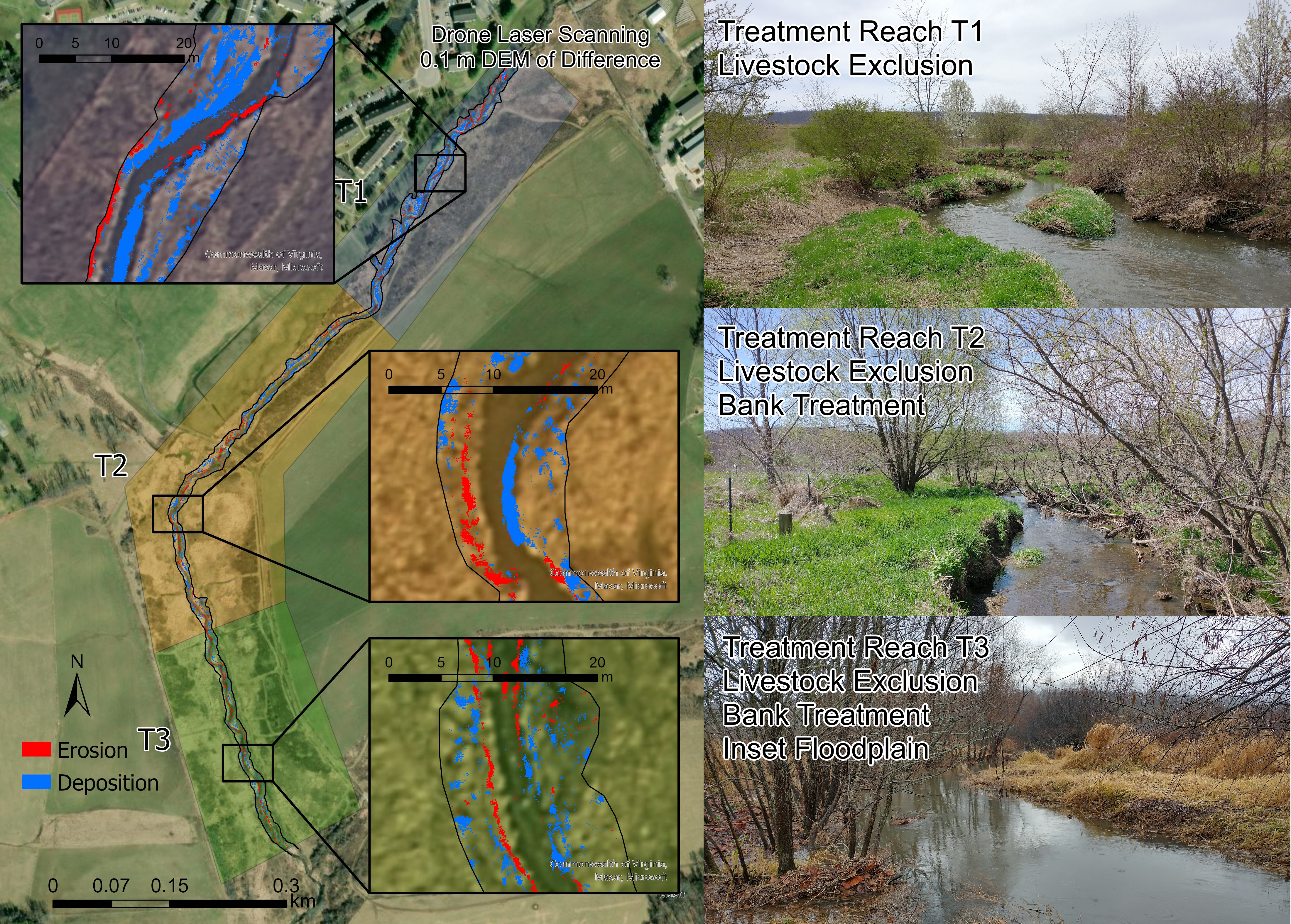
| Treatment Reach | Length (km) | Area per Length (m2/km) | Volume per Length (m3/km) | ||
|---|---|---|---|---|---|
| Erosion | Deposition | Erosion | Deposition | ||
| T1 | 0.429 | 2.683 | 11.759 | 0.914 | 4.207 |
| T2 | 0.543 | 2.707 | 1.326 | 0.775 | 0.529 |
| T3 | 0.324 | 1.481 | 1.697 | 0.422 | 0.548 |
Disclaimer/Publisher’s Note: The statements, opinions and data contained in all publications are solely those of the individual author(s) and contributor(s) and not of MDPI and/or the editor(s). MDPI and/or the editor(s) disclaim responsibility for any injury to people or property resulting from any ideas, methods, instructions or products referred to in the content. |
© 2024 by the authors. Licensee MDPI, Basel, Switzerland. This article is an open access article distributed under the terms and conditions of the Creative Commons Attribution (CC BY) license (https://creativecommons.org/licenses/by/4.0/).
Share and Cite
Resop, J.P.; Hendrix, C.; Wynn-Thompson, T.; Hession, W.C. Channel Morphology Change after Restoration: Drone Laser Scanning versus Traditional Surveying Techniques. Hydrology 2024, 11, 54. https://doi.org/10.3390/hydrology11040054
Resop JP, Hendrix C, Wynn-Thompson T, Hession WC. Channel Morphology Change after Restoration: Drone Laser Scanning versus Traditional Surveying Techniques. Hydrology. 2024; 11(4):54. https://doi.org/10.3390/hydrology11040054
Chicago/Turabian StyleResop, Jonathan P., Coral Hendrix, Theresa Wynn-Thompson, and W. Cully Hession. 2024. "Channel Morphology Change after Restoration: Drone Laser Scanning versus Traditional Surveying Techniques" Hydrology 11, no. 4: 54. https://doi.org/10.3390/hydrology11040054
APA StyleResop, J. P., Hendrix, C., Wynn-Thompson, T., & Hession, W. C. (2024). Channel Morphology Change after Restoration: Drone Laser Scanning versus Traditional Surveying Techniques. Hydrology, 11(4), 54. https://doi.org/10.3390/hydrology11040054