Article

Analysis of Landscape Pattern Evolution and Impact Factors in the Mainstream Basin of the Tarim River from 1980 to 2020

1
State Key Laboratory of Resources and Environmental Information System, Institute of Geographic Sciences and Natural Resources Research, Chinese Academy of Sciences, Beijing 100101, China
2
College of Resources and Environment, University of Chinese Academy of Sciences, Beijing 100049, China
*
Author to whom correspondence should be addressed.
Hydrology 2024, 11(7), 93; https://doi.org/10.3390/hydrology11070093
Submission received: 17 April 2024 / Revised: 18 June 2024 / Accepted: 25 June 2024 / Published: 27 June 2024

Abstract

:
The mainstream basin of the Tarim River serves as a vital ecological security barrier that prevents the merging and expansion of deserts and an important strategic corridor directly linking Qinghai and Xinjiang. With society’s development and climate change, ecological issues such as river interruption, vegetation degradation, and land desertification in the basin have notably intensified, and the ecological security is facing a critical test. Exploring the characteristics of landscape changes and their driving factors within the basin is crucial in improving the ecological environment system’s management. Based on land use data from 1980 to 2020, this study analyzed the characteristics of the spatiotemporal changes and pattern evolution of the landscape through a landscape transfer matrix and landscape pattern indices. It further revealed the impact factors of the landscape pattern through canonical correspondence analysis. The results showed that (1) in 1980–2020, the areas of desert, forest, farmland, and settlement landscapes increased, while the area of grassland landscape decreased, and the water landscape showed an “increasing–decreasing–recovery” pattern. The landscape transition types mainly included the transition from grassland to desert; mutual transitions among farmland, grassland, and forests; mutual transitions between water and grassland; and the transition from farmland to settlements. (2) The overall landscape pattern demonstrated increased fragmentation, shape complexity, and evenness with decreased aggregation. Furthermore, different landscapes exhibited distinct characteristics of landscape pattern changes; for instance, grassland landscape showed severe fragmentation, while desert landscape displayed the strongest dominance. (3) The landscape pattern was a result of the combined impact of natural and human factors, with the soil thickness (SOT), road density (ROD), annual actual evapotranspiration (AAE), population density (POD), and mean annual temperature (MAT) exhibiting significant influences. Specifically, the settlement and farmland landscapes were mainly influenced by the mean annual relative humidity (MAH), POD, GDP density (GDP), and distance to artificial water (DAW); the forest, grassland, and water landscapes were mainly influenced by the SOT, soil organic matter content (SOM), AAE, ROD, elevation (ELE), MAT, slope (SLP), and distance to natural water (DNW); and the desert landscape was mainly influenced by the DAW, DNW, SLP, AAE, SOT, SOM, and ROD. These findings can provide a scientific reference for landscape management and restoration, as well as sustainable social and economic development, in the mainstream basin of the Tarim River.

1. Introduction

The landscape, as an important component of the natural environment, plays a crucial role in maintaining an ecological balance and providing ecosystem services [1,2,3]. However, with the development of society and climate change, the balance of the landscape ecosystem is being disrupted. Environmental issues such as atmospheric changes [4,5,6], soil erosion [7,8], vegetation degradation [9,10], and biodiversity loss [11,12] are increasingly worsening, posing serious threats to regional ecological security, especially in ecologically fragile inland arid areas [13]. To address these challenges, the Land Use/Land Cover Change Scientific Research Program (LULC) was proposed in 1995, making LULC a major focus of global change research [14,15,16]. China also proposed strategic goals such as building a “beautiful China” and “upholding the integrated conservation and systematic governance of mountains, rivers, forests, farmlands, lakes, grasslands, and deserts”, aiming to promote the construction of an ecological civilization and strengthen environmental protection [17].
The landscape pattern is the result of spatial arrangements, combinations, and interactions among patches varying in size and shape [18]. Its changes significantly affect the material cycle and energy flow of the ecosystem of a region, potentially leading to adverse effects such as diminished habitat quality [19,20], heightened ecological vulnerability [21,22], and a decline in ecosystem service value [23,24]. Therefore, understanding the evolutionary characteristics of landscape patterns is crucial for the healthy development of the region [25]. Currently, the methods for the analysis of landscape patterns primarily include landscape pattern indices [26,27,28], landscape dynamic models [29,30,31], and spatial statistical analysis [32,33]. Among these, landscape pattern indices can efficiently condense landscape pattern information and reflect the spatial configuration and structural composition of the landscape, serving as a critical foundation for landscape research [18,34,35]. For example, Yang [18] utilized landscape pattern indices and found that the connectivity of the landscape in the Yangtze River Basin decreased, while the fragmentation and richness increased. Li [36] constructed a landscape ecological risk assessment model for the Selinga River Basin based on landscape pattern indices and explored the pattern characteristics of ecological risks.
The landscape pattern is influenced by various factors operating at different spatial and temporal scales. A comprehensive understanding of the impact factors of landscape patterns is of great significance in scientifically formulating ecological governance policies and implementing targeted ecological restoration measures. Current research on the causes of landscape patterns mostly centers on human factors such as the population and economy [37], as well as natural factors such as the climate and hydrology [38]. Quantitative analysis is conducted through methods like principal component analysis [39,40], multiple linear regression analysis [41,42], geographically weighted regression analysis [43,44,45], grey relation analysis [46,47], geographical detectors [21,32,48], and canonical correspondence analysis [49,50]. Among these methods, canonical correspondence analysis (CCA) is particularly effective in unraveling the complex relationships between multiple study objects and impact factors and has been widely used to examine the driving factors behind landscape patterns. Peng [51] explored the relationship between the landscape pattern and ecological factors within an agro-pastoral ecotone in Inner Mongolia based on canonical correspondence analysis and found that natural ecological factors, especially the temperature, precipitation, and altitude, had the greatest impact. Similarly, Zhao [52] studied the relationship between the landscape gradient pattern and environmental factors in the Haihe River Basin and found that the elevation, precipitation, and temperature played a decisive role in the landscape pattern at the basin scale, while the population and GDP had a significant influence in specific regions.
As a crucial region within the Tarim Basin, the mainstream basin of the Tarim River (abbreviated as “MBTR”) serves as a vital ecological security barrier that prevents the merging and expansion of deserts and an important strategic corridor directly linking Qinghai and Xinjiang. Furthermore, the MBTR is the core area for the construction of the “Silk Road Economic Belt” [53]. In recent years, with society’s development and population growth, ecological issues such as river interruption, vegetation degradation, and land desertification have notably intensified [54]. Consequently, the ecological security of the basin is facing a critical test, making it crucial to enhance the understanding of its landscape pattern. As a result, numerous scholars have extensively conducted research on ecosystem services [55,56], climate change [57,58], water resource management [59,60], and other aspects. However, limited attention has been given to the landscape pattern’s evolution and its driving factors over a long time series within the basin. Existing studies mostly focus on a simplex landscape, lacking a comprehensive understanding of the entire landscape. For example, Sun [61] established a farmland expansion model to quantify the spatiotemporal pattern of farmland landscape evolution in Yuli County, Xinjiang. Zhao [62] systematically analyzed the changes in the spatial pattern of the wetland landscape in the middle and lower reaches of the Tarim River from 1980 to 2000. Therefore, the objectives of this study are to explore the spatiotemporal evolution, internal transfer, and pattern changes of the landscape in the MBTR using a landscape transfer matrix and landscape pattern indices based on land use data from 1980 to 2020. Additionally, we aim to reveal the driving factors behind the landscape pattern in the MBTR through canonical correspondence analysis. The results provide valuable insights to promote landscape optimization, ecological improvement, and sustainable development in the MBTR.

2. Materials and Methods

2.1. Study Area

The MBTR lies on the northern edge of the Tarim Basin, located between the 39°34′ to 41°50′ N latitudes and 80°74′ to 88°55′ E longitudes, with a total area of 3.16 × 10⁴ km2. The MBTR experiences a typical temperate arid continental climate, characterized by high temperatures, aridity, substantial evaporation, and limited water resources [63]. The region exhibits a mean annual temperature of 10–11 °C, an accumulated temperature at 10 °C of 4000–4350 °C, mean annual precipitation below 50 mm, mean annual evaporation between 2300 and 3000 mm, annual sunshine hours of 2800–3100 h, and a frost-free period lasting 185–210 days [64]. The soil in the MBTR encompasses various types, including wind-sandy soil, meadow soil, tidal soil, and more. The vegetation comprises species like Populus euphratica, Tamarix chinensis, Lycium ruthenicum, Vachellia erioloba, and more [65]. Furthermore, the MBTR spans across counties and cities such as Alar, Shaya, Kuqa, Luntai, Korla, Yuli, and Ruoqiang. In 2020, there were approximately 0.52 million people in the basin, with a regional GDP of approximately RMB 37.1 billion. The geographical extent of the MBTR was determined based on the National 1:250,000 Three-Level River Basin dataset, provided by the National Cryosphere Desert Data Center (NCDC, http://www.ncdc.ac.cn, accessed on 6 June 2023).
The mainstream of the Tarim River (abbreviated as “MTR”) spans a total length of 1321 km, divided into three sections: the upstream section spans 495 km from Xiaojiake to Yingbazha; the midstream section spans 398 km from Yingbazha to Qiala; and the downstream section spans 428 km from Qiala to Taitema Lake (Figure 1) [66]. The MTR does not produce any flow and experiences a reduction in runoff volume along its course, rendering it a purely dissipative inland river in the arid zone.

2.2. Landscape Classification

Based on land use data and considering the landscape characteristics of the MBTR, this study categorized the landscape into seven types: desert landscape, grassland landscape, forest landscape, farmland landscape, water landscape, settlement landscape, and other landscape. Detailed classification information can be found in Table 1. It should be noted that the “other landscape” category primarily consists of bare land with a relatively simple landscape structure and lower landscape value, making it difficult to observe significant landscape changes. Therefore, the “other landscape” category was not considered in the specific analysis.

2.3. Data Source

The land use data, with a spatial resolution of 30 m, are obtained from the Resource and Environment Science and Data Center of the Chinese Academy of Science (REDCP, http://www.resdc.cn, accessed on 8 June 2023). The data include six first-level types (including cropland, forests, grassland, water bodies, built-up land, and unused land) and 25 second-level types, with the combined accuracy for the first-level and second-level types exceeding 90% [67]. In the analysis of the driving factors of the landscape pattern, data on the mean annual temperature, mean annual precipitation, mean annual relative humidity, elevation, population density, and GDP density, with a spatial resolution of 1 km, are provided by REDCP. Additionally, the soil organic matter content data come from the National Tibetan Plateau Data Center (TPDC, https://data.tpdc.ac.cn/, accessed on 15 June 2023). The soil thickness data come from the National Earth System Science Data Center (NESSDC, http://www.geodata.cn, accessed on 18 June 2023). The annual actual evapotranspiration data come from the Harvard Dataverse (https://dataverse.harvard.edu/, accessed on 18 June 2023). Finally, the natural water, artificial water, and road data are provided by the National Cryosphere Desert Data Center (NCDC, http://www.ncdc.ac.cn, accessed on 20 June 2023). The data sources are shown in Table 2.

2.4. Research Methodology

2.4.1. Landscape Pattern Indices

The landscape pattern indices generally include three levels: the patch level, class level, and landscape level [18]. According to the characteristics of the study area and research requirements, this study mainly analyzed the landscape pattern at the class and landscape levels. Considering the ecological significance of each index, eleven indices were selected, which mainly corresponded to the fragmentation, dominance, shape complexity, aggregation, and diversity of the landscape (Table 3). The detailed definitions and formulas of these landscape pattern indices can be found in Yang [18], Yu [34], and Zhang [68].

2.4.2. Canonical Correspondence Analysis

Canonical correspondence analysis (CCA) is a nonlinear multivariate direct gradient analysis method that combines correspondence analysis with multiple regression analysis. In CCA, the grid square is used as the analysis unit. According to the principles of landscape ecology, the scale of division of the grid units is usually determined as two to five times the average area of the patches in the study area [69]. Based on the actual size of the landscape patches in the MBTR and the spatial resolution of the land use data and impact factors, the grid square size was set to 6 km, generating 707 grid squares. Furthermore, two data matrices were required: the impact factor matrix and the landscape pattern matrix. The impact factors were considered from two aspects, natural factors and human factors, as shown in Table 4. Impact factors within the grid squares were assigned according to the average value. As for the landscape pattern values, this study took the landscape area shares of six landscape types within the grid squares as the quantitative indicators.
The ordination diagram generated by CCA can be used to visualize the main distribution features of the landscape pattern along the impact factors, as well as the importance of these factors. The CCA ordination diagram is constructed and interpreted as follows: arrows represent the impact factors, and triangles represent the landscape area shares; the length of the arrows represents the degree of influence of the impact factors on the landscape pattern, with a longer length indicating a greater influence; the direction of the arrows represents the maximum change in the impact factors; the distances of the triangles represent similarities in the distributions of landscape types. In addition, the order of the triangles projected onto a specific arrow reveals the optimal ranking of the landscapes regarding the impact factor [70].

2.4.3. Bivariate Local Spatial Autocorrelation

Bivariate local spatial autocorrelation (also known as bivariate LISA) was used to explore the spatial agglomeration effect of farmland expansion and socioeconomic development (population and GDP growth) at the grid scale (consistent with the grid in CCA). A bivariate LISA map provides four types of agglomeration: high–high, low–low, low–high, and high–low [71]. The bivariate LISA statistics can be calculated based on the following equation [71,72,73]:
I i = Z x i j = 1 , j i N W i j Z y j
where I i is the local Moran’s I (LISA); x and y are two variables of interest (here, they refer to farmland expansion and population or GDP growth) for grid i and neighborhood j, respectively. Z x and Z y are the standardized z-scores for variables x and y, respectively. W i j is the weight matrix that defines the structure of the neighborhood. We use a first-order queen contiguity matrix, where w i j   =  1 if the adjacent grid j shares a common border with the i-th grid, and w i j   =  0 otherwise.

3. Results and Analysis

3.1. Landscape Evolution Analysis

3.1.1. Characteristics of Landscape’s Spatiotemporal Evolution

The landscapes of the MBTR changed significantly from 1980 to 2020 (Figure 2, Table 5 and Table 6). The desert landscape initially expanded, with its area share increasing from 31.43% of the total area of the MBTR in 1980 to 37.00% in 2010, before slightly decreasing to 36.49% by 2020. The desert increased by 1597 km2 overall, primarily attributed to desertification in the middle and lower reaches of the basin. The most significant changes occurred in 1990–2000 and 2000–2010, with the change rates of 6.15% and 10.77%, respectively. The grassland landscape continuously decreased from 46.91% in 1980 to 32.61% in 2020, shrinking by 4518 km2. The decline mainly occurred on the sides of the upper and middle reaches of the MBTR and in the east of the downstream region. The degradation was particularly serious in 1990–2000 and 2000–2010, with the change rates of −10.20% and −19.78%, respectively. The forest landscape displayed an overall increasing trend, expanding by 523 km2, notably outward from the river channel, particularly in the upper reaches. The increase rates in 1990–2000 and 2000–2010 were 6.95% and 7.10%, respectively. The farmland landscape continued to expand by 2581 km2, with its area share increasing from 4.27% to 12.44%. The expansion area was mainly concentrated in Alaer, the northern area of Shaya, the southern area of Kuqa, and the sides of the middle reaches of the MBTR. Notably, the change rate soared to 90.22% in 2000–2010. The water landscape showed fluctuating changes, with an overall decrease of 182 km2. This fluctuation involved an increase in 1990–2000 due to expansion in the lakes, wetlands, and reservoirs downstream, and a shrinkage in 2000–2010 in the middle and lower reaches of the river. The settlement landscape grew from 56 km2 in 1980 to 92 km2 in 2020, mainly due to the expansion of Alaer.

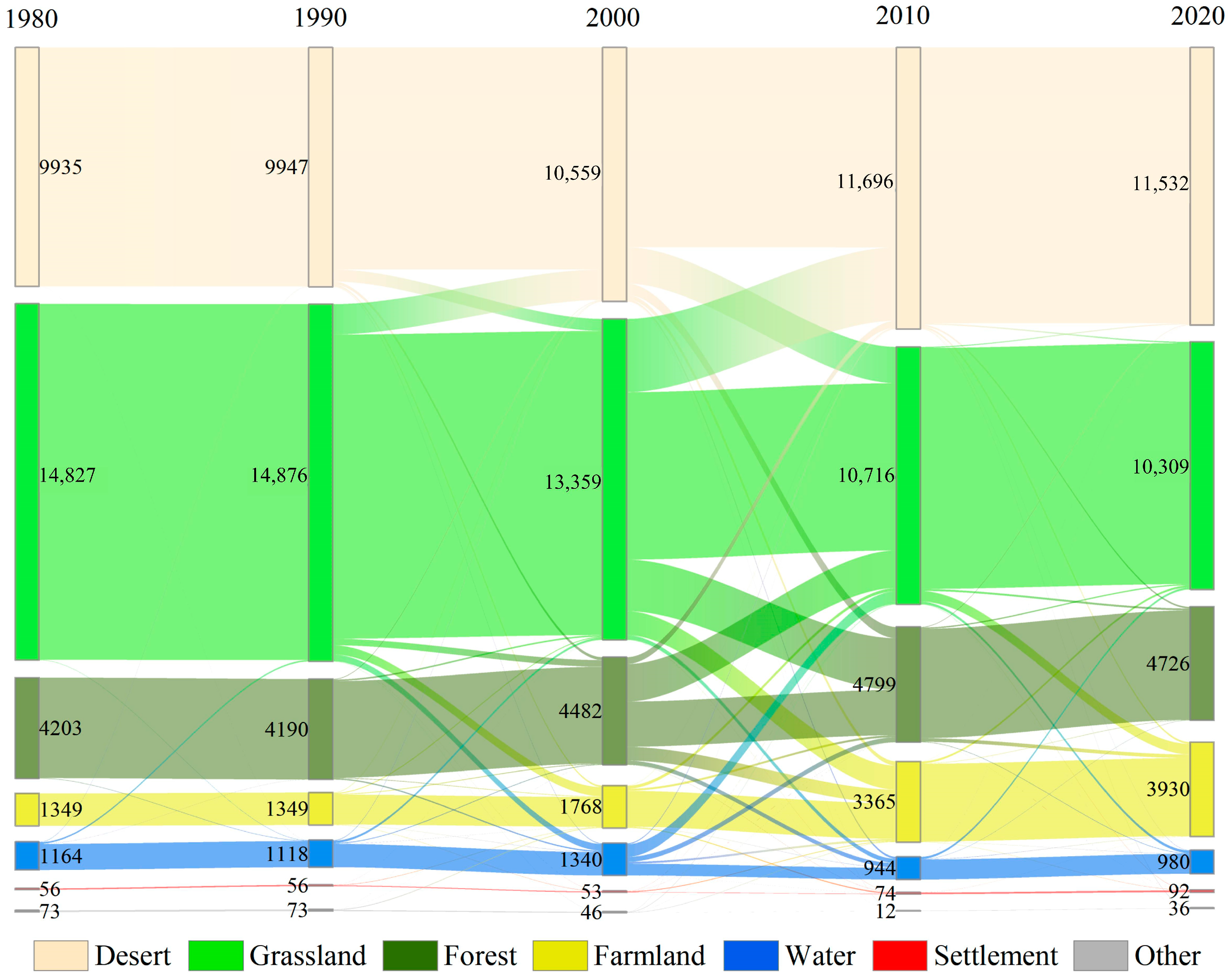
3.1.2. Characteristics of Landscape Transfer

Over time, the various landscapes in the MBTR have experienced significant transitions. This study employed a landscape transfer matrix to describe the quantity and direction of the transformations among the different landscapes. These changes were further visualized using a Sankey diagram, as seen in Figure 3. The increased area of the desert landscape mainly came from the grassland. It was most obvious in 1990–2000 and 2000–2010, with 1267 km2 and 3055 km2 of grassland transferred to the desert, accounting for 94.84% and 90.01% of the total transition to desert, respectively. The grassland landscape decreased significantly, mainly transferred to the desert, farmland, and forest landscapes. In 1990–2000, 2218 km2 of grassland was converted, primarily to desert, accounting for 57.12%, followed by farmland, water, and forests, accounting for 42.47% in total. In 2000–2010, the grassland degradation intensified, with the transfer out of 6396 km2, notably 47.76% to desert, 33.58% to forests, and 15.63% to farmland. In 2010–2020, the grassland degradation showed an improvement, with 687 km2 converted, primarily to farmland, with 63.75%. The slight increase in the forest landscape was primarily due to the transition of grassland. In 1990–2000, the forest area increased slightly, mostly being converted from grassland and desert. In 2000–2010, a drastic transition occurred between forests and grassland, with 1561 km2 of forests transforming into grassland and 2148 km2 of grassland transforming into forests. Regarding farmland expansion, it was mainly due to the transition from grassland and forests. In 1990–2000, 528 km2 of land was transferred to farmland, with 72.92% from grassland. In 2000–2010, 1875 km2 of land was transferred to farmland, with 53.33% and 30.29% from grassland and forests, respectively. Meanwhile, in 2010–2020, 686 km2 of land was transferred to farmland, with 63.85% and 22.01% from grassland and forests, respectively. The water landscape mainly underwent mutual transitions with the grassland landscape, showing an overall reduction in area. Grassland converted to water amounted to 284 km2 in 1990–2000, while water converted to grassland and forests amounted to 527 km2 and 207 km2, respectively, in 2000–2010. The settlement landscape increased slightly, mainly due to the transition from farmland.

3.2. Landscape Pattern Analysis

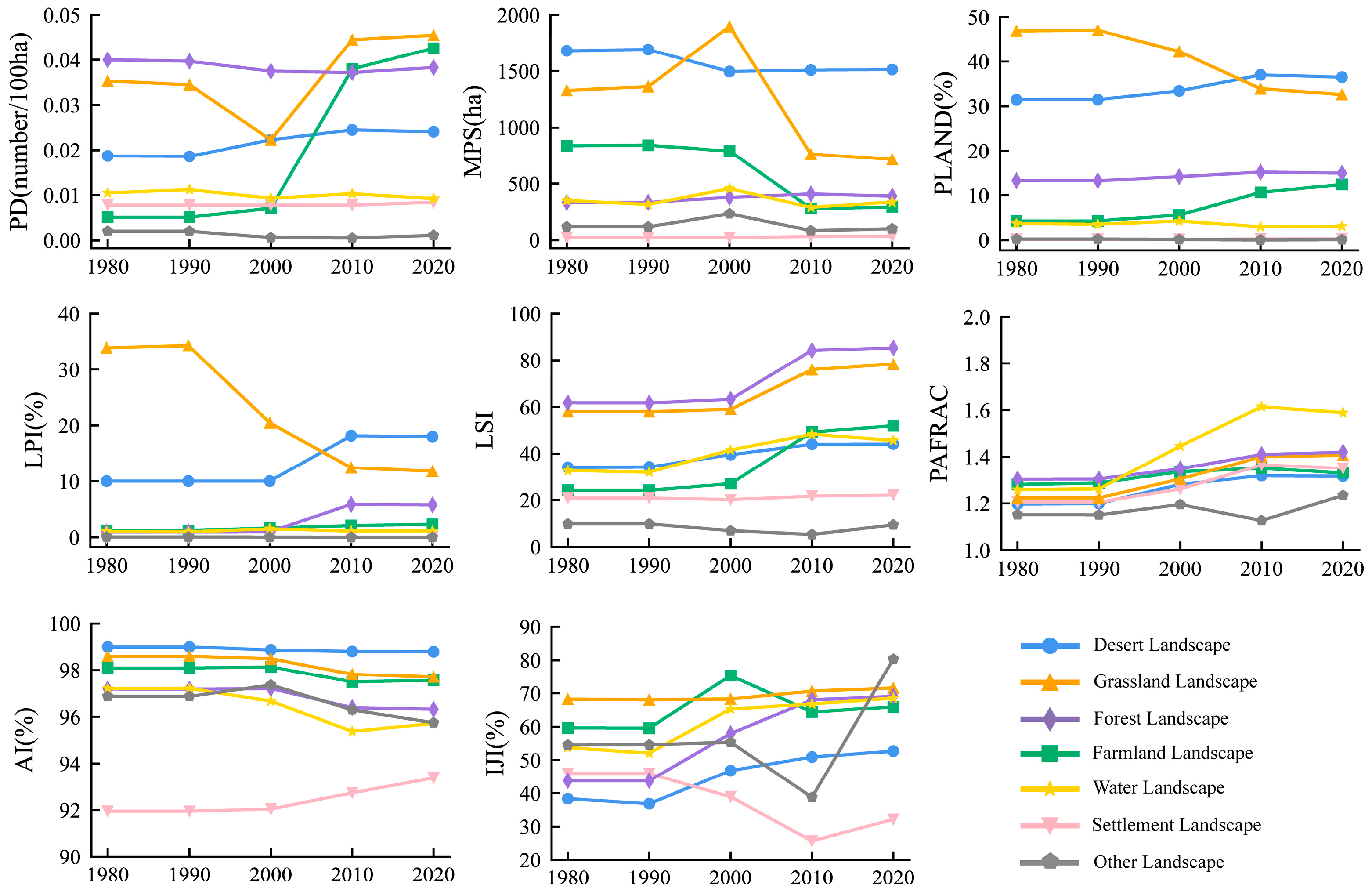
3.2.1. Landscape Pattern Analysis at Class Level

The changes in the landscape pattern indices at the class level in the MBTR from 1980 to 2020 are shown in Figure 4. In terms of fragmentation characteristics, the patch density (PD) increased and the mean patch size (MPS) decreased in both the desert and farmland landscapes, with a more pronounced change observed in farmland. In the grassland and water landscapes, the PD decreased and then increased, and the MPS increased and then decreased. The PD of the forest landscape decreased slightly and the MPS increased slightly. The PD and MPS of the settlement landscape showed little variation. It can be seen that all landscapes, except for forests and settlements, tended towards fragmentation after 2000, with the most significant changes occurring between 2000 and 2010.
Regarding the dominance characteristics, grassland and desert exhibited the highest percentage of landscape (PLAND) and the largest patch index (LPI), signifying strong landscape dominance. However, the PLAND and LPI of grassland decreased, while those of desert increased. By 2020, desert surpassed grassland to become the dominant landscape. The PLAND and LPI of the farmland, settlement, and forest landscapes increased, indicating an enhancement in landscape dominance, while those of water fluctuated, showing a slight overall decrease.
The shape complexity, as measured by the landscape shape index (LSI) and perimeter-area fractal dimension (PAFRAC), showed an increasing trend in all landscapes from 1980 to 2020, with the most significant change occurring in 1990–2010. This trend indicated that all landscape patches tended to become more complex and irregular. Notably, the PAFRAC of farmland and settlements marginally decreased in 2010–2020, indicating that the patch shapes became simpler due to activities such as rural construction management and farmland management, after experiencing a rapid development period of shape complexity.
In terms of the aggregation characteristics, from 1980 to 2020, the aggregation index (AI) of the desert, forest, water, and grassland landscapes exhibited a consistent decline, while the interspersion juxtaposition index (IJI) showed an overall increase, most notably in 1990–2010. This trend stemmed from the significant transitions among desert, forests, water, and grassland, leading to an enhanced landscape mosaic and patch fragmentation. The AI of farmland decreased, and the IJI increased followed by a decline. Initially, the expansion of farmland was arbitrary, leading to reduced aggregation and increased adjacency with other landscapes. However, with the implementation of intensive agricultural management practices, the aggregation of farmland began to recuperate. Meanwhile, the AI of settlements increased continuously, with the IJI initially decreasing and then rising. This shift occurred because the settlement landscape initially became denser by filling in existing gaps and later expanded outward, establishing closer connections with adjacent landscapes. Overall, the aggregation of all landscapes, with the exception of the settlement landscape, has decreased.

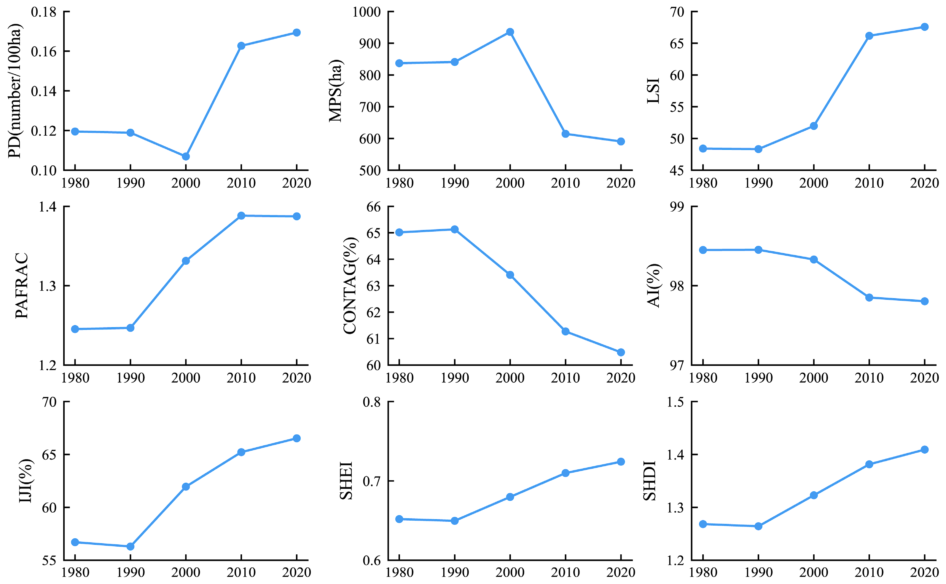
3.2.2. Landscape Pattern Analysis at Landscape Level

The changes in the landscape pattern indices at the landscape level in the MBTR from 1980 to 2020 are shown in Figure 5. From 1980 to 2020, the PD initially decreased and then increased, while the MPS initially increased and then decreased, both changing around 2000, with the most significant changes occurring in 2000–2010. This indicated a relatively stable ecological environment before 2000, contrasted by intensified landscape fragmentation after 2000. The LSI and PAFRAC displayed consistent growth, especially evident in 1990–2010, indicating heightened complexity in the patch shapes. Concurrently, the AI and contagion (CONTAG) decreased, whereas the IJI increased, indicating that the aggregation and connectivity of the overall landscape decreased and the probability of adjacency between various landscapes increased. These changes primarily emerged due to substantial transitions among landscapes, resulting in their increased interpenetration and fragmentation. Moreover, the increasing trends of Shannon’s diversity index (SHDI) and Shannon’s evenness index (SHEI) suggested increased landscape diversification and evenness. These changes can be explained by the decreased proportion of grassland, coupled with the increased proportions of forests, farmland, and settlements, contributing to more balanced development among the diverse landscapes.

3.3. Analysis of Factors Influencing Landscape Pattern

From the previous analysis, it can be seen that the landscape changes in 1980–1990 and 2010–2020 were relatively minor, while significant landscape changes occurred around the year 2000. Therefore, to avoid redundant analyses, this study selected the years 1980, 2000, and 2020 to analyze the impact factors of the landscape pattern.

3.3.1. Feasibility Analysis of CCA

In this study, a detrended correspondence analysis (DCA) was initially conducted on the landscape area shares. According to the ordination results, if the length of the ordination axis with the longest gradient is less than 3, a linear model is optimal; if it exceeds 4, a single-peak model is optimal; and if it equals 3 to 4, both linear and single-peak models are suitable [50]. The lengths of the first ordination axis for the landscape area shares in 1980, 2000, and 2020 were 3.20, 3.02, and 3.07, respectively, indicating suitability for the CCA method.
Furthermore, the statistical data for each ordination axis in CCA are shown in Table 7. In 1980, 2000, and 2020, the first two ordination axes collectively accounted for 88.76%, 88.83%, and 82.30% of the relationship between the landscape area shares and impact factors, indicating that the majority of information concerning their relationship can be obtained from these two axes. Meanwhile, the correlation coefficients between the landscape area shares and impact factors on the first ordination axis were 0.81, 0.86, and 0.95, respectively, while they were 0.67, 0.69, and 0.71 on the second ordination axis, demonstrating a strong correlation. In addition, Monte Carlo permutation tests were conducted on the first ordination axes and all ordination axes, and the p-values were all 0.001 (Table 8), reaching a highly significant level. All of the above results indicate that CCA can effectively explain the relationship between the landscape pattern characteristics and impact factors over the three years.

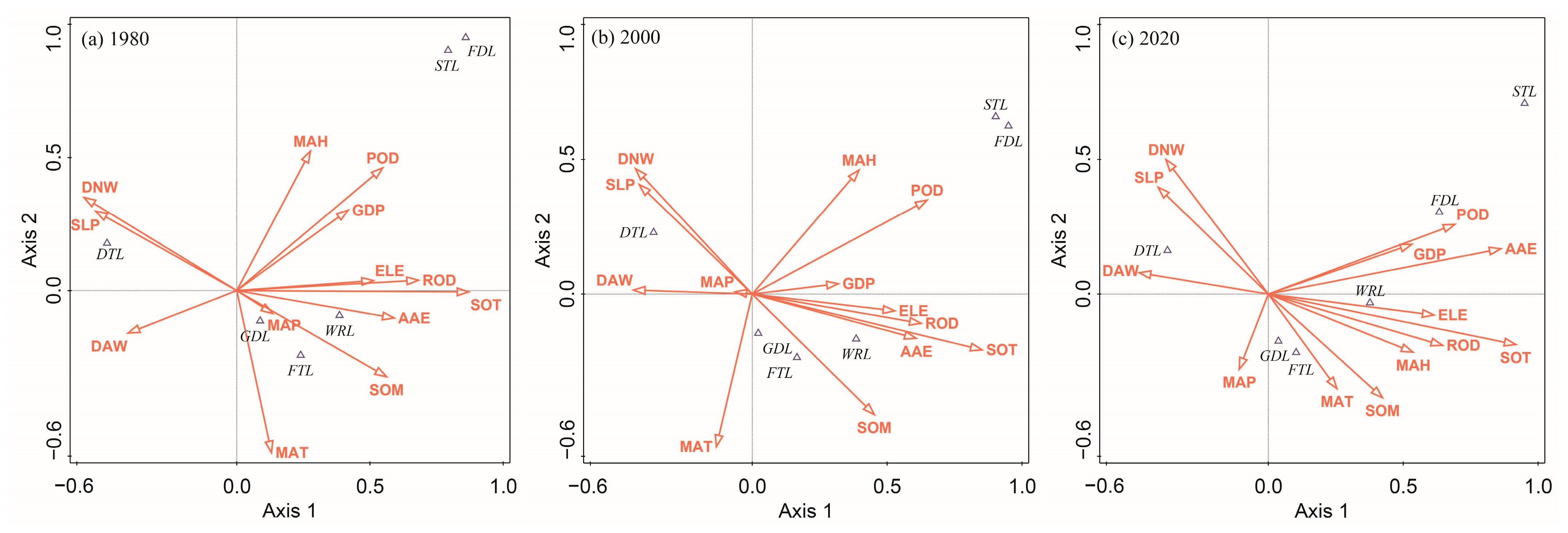
3.3.2. CCA of the Landscape Area Shares and Impact Factors

Figure 6 displays the correlations between 13 impact factors and the landscape area shares of six landscape types in 1980, 2000, and 2020. The settlement and farmland landscapes were mainly positively correlated with the mean annual relative humidity (MAH), population density (POD), and GDP density (GDP), but negatively correlated with the distance to artificial water (DAW). Farmland, as an artificial landscape, heavily relies on water and is often concentrated in densely populated areas with accessible irrigation. The forest, grassland, and water landscapes displayed positive correlations with the soil thickness (SOT), soil organic matter content (SOM), annual actual evapotranspiration (AAE), road density (ROD), elevation (ELE), and mean annual temperature (MAT), while they were negatively correlated with the slope (SLP) and distance to natural water (DNW). Regions with higher soil organic matter content, abundant water resources, moderate temperatures, and gentle terrain favor the growth of forests and grasslands [10]. The desert landscape exhibited a clear positive correlation with the DAW, DNW, and SLP, while showing a negative correlation with the AAE, SOT, SOM, and ROD.
Furthermore, the proximity between the farmland and settlement landscapes indicated their spatial closeness, making them convenient for cultivation and the provision of food supplies for residents. Similarly, the proximity among the grassland, forest, and water landscapes was primarily due to grassland and forests’ reliance on water sources, fostering their coexistence.
The relationships between the landscape types and various impact factors varied over time (Table 9). In 1980, 2000, and 2020, the SOT emerged as the most influential factor for the landscape pattern, exhibiting correlation coefficients of 0.87, 0.85, and 0.92 with the first axis, followed by the ROD (0.68, 0.63, 0.65), AAE (0.59, 0.61, 0.86), and POD (0.55, 0.65, 0.69). Moreover, the MAT displayed the strongest correlation with the second axis, with correlation coefficients of −0.61, −0.56, and −0.35, respectively. Over time, the correlations of the SOT, AAE, and POD have strengthened, while that of the MAT has weakened, with the correlation of the ROD remaining stable.

4. Discussion

4.1. Driving Factors of Landscape Pattern

The landscape pattern is jointly influenced by multiple factors, such as the population, economy, soil, and hydrology, with different landscapes being affected by distinct factors. In this study, we identified a strong positive correlation between the distribution of the farmland and settlement landscapes and the POD and GDP. The growth in the population and economy has promoted the expansion of the farmland and settlement landscapes, which is consistent with previous research [74,75,76]. Our statistics indicated that, from 1980 to 2020, the farmland and settlement landscapes in the MBTR showed an increasing trend, particularly with a significant increase in farmland of 2582 km2. Additionally, the population in the MBTR increased by 0.23 million people, and the GDP increased by RMB 1.53 million. The results of the bivariate local spatial autocorrelation analysis further indicated that (Figure 7), over the past two decades, the MBTR’s farmland expansion exhibited obvious spatial aggregation effects with population growth and economic development, with I-values of 0.431 and 0.373, respectively. Specifically, areas with high–high agglomeration of farmland expansion and population growth were mainly distributed in the upstream areas of Alar and Kuqa. Conversely, areas with the relatively slow expansion of farmland and population growth were mainly distributed in the middle and lower reaches, and areas with the relatively slow expansion of farmland and economic development were primarily distributed in the central part of the basin.
In addition, the distribution of the forest, grassland, and water landscapes was primarily influenced by the soil and hydrological conditions. This study delved into the differences in the landscape distribution under various soil and hydrological conditions. The impact factors were classified into five levels by natural breaks: low (I), relatively low (II), medium (III), relatively high (IV), and high (V). Furthermore, an overlay analysis was conducted on the spatial distribution of the landscapes and impact factors to reflect the distribution differences of the landscapes under different gradings of the impact factors. The results indicated that the distribution proportion of the forest landscape was the highest with the SOT, SOM, and AAE under levels III and IV (Figure 8), and the distribution proportion of the grassland landscape was the highest with the SOT under level III, SOM under level V, and AAE under level II (Figure 9). It can be observed that regions with a high soil thickness, high soil organic matter content, and abundant water resources are more conducive to the growth of forest and grassland landscapes. Peng [10] suggested that areas with higher groundwater levels, a closer proximity to rivers, and moderate soil conditions are more suitable for the distribution of forest landscape. Moreover, the optimal values of the SOT, SOM, and AAE decreased sequentially for water, forest, and grassland landscapes, which suggests that the formation and maintenance of water landscape often requires a better soil structure and favorable water supply conditions, while the forest landscape has higher requirements for its growth environment compared to the grassland landscape.
The desert landscape was mostly distributed on the edges of the upper and middle reaches of the MBTR, as well as in the lower reaches. These areas were far from water sources, with poor soil conditions and minimal human interference, making them more prone to land desertification. Particularly in 1990–2010, the expansion of the desert landscape was significant, mainly due to the rapid cultivation in the upper and middle reaches and the increase in agricultural water usage, which directly led to a decrease in the groundwater level downstream, exacerbating grassland degradation and land desertification. This finding is consistent with the research results of Wang [77].
Studies have identified a warming trend in the MBTR since 1980, noting a rise in the average spring temperature of 0.52 °C per decade and a rise in dryness during spring and winter of 22.14 and 14.01 per decade, respectively [78]. An optimal temperature is conducive to the growth of forest and grassland landscapes. As the temperatures rose, the influence of the temperature on the landscapes gradually weakened, while the demand for water resources by the landscapes intensified. Meanwhile, human activities can affect the shaping types and evolution rates of the landscape. With the acceleration of urbanization and the intensification of human activities, the impact of the population density on the landscapes gradually strengthened.

4.2. Impact of Policies on Landscape Pattern

The evolution of the landscape pattern is influenced by numerous factors. In addition to the selected natural and human factors, policy formulation, technological development, and enhanced landscape conservation awareness will all have direct or indirect impacts on the landscape evolution of the MBTR. Among them, the influence of policies is particularly significant, but it is difficult to quantify. Therefore, this paper discusses the impact of policy factors.
With the commencement of the reform and opening up of China, the financial support for agriculture in Xinjiang has continuously increased, and human activities have gradually intensified. The small-scale land reclamation movement began in 1988 [79]. In 1995, Xinjiang proposed the “One Black and One White” development strategy. (“One Black” refers to petroleum and “one white” refers to cotton. Xinjiang has favorable natural conditions for cotton cultivation. After receiving support from national policies and funds, the area of cotton cultivation has rapidly expanded.) It encouraged individuals and collectives to cultivate land [80]. This initiative triggered extensive land reclamation efforts, resulting in the clearance of vast areas of windbreak grassland, shrubs, and forests, causing a sharp reduction in grassland and the exacerbation of land desertification. Concurrently, the government strongly promoted the development of forestry and fruit industries, leading to expanded artificial forest land. Additionally, the implementation of the “Western Development Strategy” in 2000 led to a rapid increase in population and land demands, accelerating the expansion of the settlement and farmland landscapes. However, the expanded farmland and increased agricultural activities led to the excessive exploitation and irrational distribution of the water resources, reducing the ecological water usage and exacerbating the ecological environment’s degradation in the MBTR [77,81]. Under such circumstances, the Tarim River Basin Comprehensive Management Project began in 2001. Through the Ecological Water Conveyance Project [82], multiple ecological water conveyances were carried out in the middle and lower reaches, aiming to promote the recovery of the groundwater and counteract the lake’s desiccation and vegetation degradation. Despite these efforts, the long-term ecological deterioration persisted due to societal, economic, and natural constraints, and phenomena like grassland degradation and lake desiccation remained, aligning with the research results of Sun [83]. Furthermore, the construction of water conservancy facilities such as river embankments reduced some natural flood spillways like distributaries and bay flows, resulting in reduced water areas. In 2010–2020, the implementation of ecological water conveyance and water-saving irrigation projects began to show positive impacts, such as increasing water areas, restraining grassland degradation, and reducing desert areas. Simultaneously, the development of oasis agriculture further enhanced the cultivation of arable land. These findings are consistent with the conclusions drawn by Wang [84], Sun [85], and Hou [86].

4.3. Suggestions to Improve Ecological Conditions of MBTR

Over the past 40 years, with the development of society and the economy, artificial landscapes have rapidly developed and gradually stabilized. However, natural landscapes, especially grassland landscape, have been severely damaged. Based on the research in this study, some suggestions for landscape management and protection in the MBTR are proposed.
(1) It is necessary to maintain the sustainable development of forests and pay attention to the protection of grassland. Forests and grassland are the most important factors in maintaining ecological stability [36]. Implementing planned irrigation regularly and selecting suitable species can strengthen vegetation restoration and protection.
(2) It is necessary to control the scale of farmland and promote water-saving irrigation measures. Water resources are a fundamental condition for the achievement of sustainable development in the MBTR. The expansion of farmland in the source stream area and the increase in agricultural water use have led to a decrease in water transport in the MBTR, resulting in vegetation death and land desertification. Therefore, to ensure the healthy development of the ecological environment in the basin, it is necessary to reasonably control the development area of farmland, promote agricultural water-saving irrigation technology, and improve the agricultural water use efficiency.
(3) It is necessary to strengthen ecological restoration projects. Since 2000, the Ecological Water Conveyance Project has been implemented [66]. After 2010, the positive effect of this project began to emerge, with vegetation degradation and land desertification slowing down and water areas increasing. Additionally, there are other ecological projects, such as the Desertification Control Project, the Grain for Green Project [71], and the Natural Forest Protection Project, which have made positive contributions to the ecological restoration of the MBTR.

4.4. Limitations and Prospects

4.4.1. Determination of Optimal Landscape Scale

Changes in spatial scale can significantly influence the outcomes of landscape pattern research. When dividing the study area for landscape pattern analysis, using a large division scale may result in the loss of the finer details of the landscape pattern. Conversely, adopting a small division scale can lead to the obscuration or neglect of crucial information due to the overwhelming amount of data within each grid [87,88]. Knowing this, we set the grid size to 6 km based on the principle of 2–5 times the average area of landscape patches and the spatial resolutions of different data. However, this was not sufficient. To mitigate the impact of the spatial scale on the results, additional research is needed to understand how the landscape scale affects the relationship between the landscape pattern and influencing factors, as well as to determine the optimal landscape scale for landscape pattern analysis within the range of 2–5 times the average area of patches in the MBTR.

4.4.2. Selection and Expansion of Impact Factors

This study selected representative influencing factors based on natural and human factors to analyze the driving forces of the landscape pattern in the MBTR. Natural factors generally play a decisive role in the formation and distribution of landscape types over a large range and long period of time, while human factors usually have a direct impact on the evolution and development of the landscape pattern within a small area and in a short period of time. However, the relationship between the landscape pattern and influencing factors has not been fully revealed due to the limited selection of factors and their complex interactions. Therefore, additional factors, such as policy factors, cultural factors, and biological factors, and diverse analysis methods are required to comprehensively consider the relationship between the landscape pattern and the influencing factors in further studies.

5. Conclusions

This study examined the spatiotemporal changes and pattern characteristics of the landscape in the MBTR from 1980 to 2020 and revealed the impact of natural and human factors on the landscape pattern. Our results showed that (1) from 1980 to 2020, the areas of the desert, forest, farmland, and settlement landscapes in the MBTR increased, with the farmland showing the greatest increase of 2582 km2, while the area of the grassland landscape continuously decreased by 4519 km2 and the water landscape showed an “increasing–decreasing–recovery” pattern, peaking at 1340 km2 in 2000. The main types of landscape transitions in the MBTR included the transition from grassland to desert; mutual transitions among farmland, grassland, and forests; mutual transitions between water and grassland; and the transition from farmland to settlements. (2) From 1980 to 2020, the overall landscape pattern exhibited an increase in patch fragmentation, shape complexity, and evenness, alongside a decrease in aggregation. Specifically, the fragmentation, dominance, and shape complexity of the desert and farmland landscapes increased, while their aggregation decreased. The grassland landscape showed increased fragmentation and shape complexity, but decreased dominance and aggregation. The forest landscape experienced decreased fragmentation and aggregation, along with increased dominance and shape complexity. The fragmentation of the water landscape showed a trend of initially decreasing before increasing, with the dominance showing the opposite trend. It also experienced increased shape complexity and decreased aggregation. The settlement landscape exhibited decreased fragmentation and increased shape complexity, dominance, and aggregation. (3) The landscape pattern in the MBTR was influenced by a combination of natural and human factors, primarily the SOT, ROD, AAE, POD, and MAT. Specifically, the settlement and farmland landscapes were mainly influenced by the MAH, POD, GDP, and DAW; the forest, grassland, and water landscapes were mainly influenced by the SOT, SOM, AAE, ROD, ELE, MAT, SLP, and DNW; and the desert landscape was mainly influenced by the DAW, DNW, SLP, AAE, SOT, SOM, and ROD.
The landscape in the MBTR is vulnerable and highly sensitive to human interference and environmental changes. This study explored the impact of the natural environment and human activities on the landscape pattern and offers specific recommendations for landscape optimization and ecological improvement. In the future, we will focus on the changes and development of the landscape pattern at different spatial scales, as well as the relationship between the landscape pattern and more comprehensive influencing factors.

Author Contributions

Conceptualization, L.J.; data curation, Y.L.; formal analysis, Y.L.; funding acquisition, L.J.; investigation, Y.L.; methodology, Y.L.; project administration, L.J.; resources, L.J.; software, Y.L.; supervision, L.J.; validation, Y.L.; visualization, Y.L.; writing—original draft, Y.L.; writing—review and editing, L.J. All authors have read and agreed to the published version of the manuscript.

Funding

This research was funded by the Third Xinjiang Scientific Expedition Program, grant number 2021xjkk0303.

Data Availability Statement

The data generated and analyzed during this study are available from the corresponding author by request.

Acknowledgments

The authors appreciate the detailed comments from the editor and the anonymous reviewers.

Conflicts of Interest

The authors declare no conflicts of interest.

References

  1. Schaubroeck, T.; Deckmyn, G.; Giot, O.; Campioli, M.; Vanpoucke, C.; Verheyen, K.; Rugani, B.; Achten, W.; Verbeeck, H.; Dewulf, J.; et al. Environmental impact assessment and monetary ecosystem service valuation of an ecosystem under different future environmental change and management scenarios; a case study of a Scots pine forest. J. Environ. Manag. 2016, 173, 79–94. [Google Scholar] [CrossRef]
  2. Sannigrahi, S.; Chakraborti, S.; Joshi, P.K.; Keesstra, S.; Sen, S.; Paul, S.K.; Kreuter, U.; Sutton, P.C.; Jha, S.; Dang, K.B. Ecosystem service value assessment of a natural reserve region for strengthening protection and conservation. J. Environ. Manag. 2019, 244, 208–227. [Google Scholar] [CrossRef]
  3. Chen, B.; Jing, X.; Liu, S.; Jiang, J.; Wang, Y. Intermediate human activities maximize dryland ecosystem services in the long-term land-use change: Evidence from the Sangong River watershed, northwest China. J. Environ. Manag. 2022, 319, 115708. [Google Scholar] [CrossRef]
  4. Ziter, C.D.; Pedersen, E.J.; Kucharik, C.J.; Turner, M.G. Scale-dependent interactions between tree canopy cover and impervious surfaces reduce daytime urban heat during summer. Proc. Natl. Acad. Sci. USA 2019, 116, 7575–7580. [Google Scholar] [CrossRef]
  5. Xiao, R.; Cao, W.; Liu, Y.; Lu, B. The impacts of landscape patterns spatio-temporal changes on land surface temperature from a multi-scale perspective: A case study of the Yangtze River Delta. Sci. Total Environ. 2022, 821, 153381. [Google Scholar] [CrossRef]
  6. Das, N.; Mondal, P.; Sutradhar, S.; Ghosh, R. Assessment of variation of land use/land cover and its impact on land surface temperature of Asansol subdivision. Egypt. J. Remote Sens. Space Sci. 2021, 24, 131–149. [Google Scholar] [CrossRef]
  7. Chen, C.; Zhao, G.; Zhang, Y.; Bai, Y.; Tian, P.; Mu, X.; Tian, X. Linkages between soil erosion and long-term changes of landscape pattern in a small watershed on the Chinese Loess Plateau. Catena 2023, 220, 106659. [Google Scholar] [CrossRef]
  8. Song, S.; Yu, D.; Li, X. Impacts of changes in climate and landscape pattern on soil conservation services in a dryland landscape. CATENA 2023, 222, 106869. [Google Scholar] [CrossRef]
  9. Nan, Z. The grassland farming system and sustainable agricultural development in China. Grassl. Sci. 2005, 51, 15–19. [Google Scholar] [CrossRef]
  10. Peng, Y.; He, G.; Wang, G. Spatial-temporal analysis of the changes in Populus euphratica distribution in the Tarim National Nature Reserve over the past 60 years. Int. J. Appl. Earth Obs. Geoinf. 2022, 113, 103000. [Google Scholar] [CrossRef]
  11. Ceballos, G.; Ehrlich, P.R.; Raven, P.H. Vertebrates on the brink as indicators of biological annihilation and the sixth mass extinction. Proc. Natl. Acad. Sci. USA 2020, 117, 13596–13602. [Google Scholar] [CrossRef] [PubMed]
  12. Yang, S.; Yuan, Z.; Ye, B.; Zhu, F.; Chu, Z.; Liu, X. Impacts of landscape pattern on plants diversity and richness of 20 restored wetlands in Chaohu Lakeside of China. Sci. Total Environ. 2024, 906, 167649. [Google Scholar] [CrossRef] [PubMed]
  13. Wang, G.; Ran, G.; Chen, Y.; Zhang, Z. Landscape Ecological Risk Assessment for the Tarim River Basin on the Basis of Land-Use Change. Remote Sens. 2023, 15, 4173. [Google Scholar] [CrossRef]
  14. Salazar, A.; Baldi, G.; Hirota, M.; Syktus, J.; McAlpine, C. Land use and land cover change impacts on the regional climate of non-Amazonian South America: A review. Glob. Planet. Chang. 2015, 128, 103–119. [Google Scholar] [CrossRef]
  15. Han, Y.; Yu, D.; Chen, K. Evolution and Prediction of Landscape Patterns in the Qinghai Lake Basin. Land 2021, 10, 921. [Google Scholar] [CrossRef]
  16. Maimaitiyiming, M.; Ghulam, A.; Tiyip, T.; Pla, F.; Latorre-Carmona, P.; Halik, Ü.; Sawut, M.; Caetano, M. Effects of green space spatial pattern on land surface temperature: Implications for sustainable urban planning and climate change adaptation. ISPRS J. Photogramm. Remote Sens. 2014, 89, 59–66. [Google Scholar] [CrossRef]
  17. Cheng, J.; You, Z. Scientific connotation and practical paths about the principle of ‘taking mountains, rivers, forests, farmlands, lakes, and grasslands as a life community’. China Popul. Resour. Environ. 2019, 29, 1–6. [Google Scholar]
  18. Yang, H.; Zhong, X.; Deng, S.; Nie, S. Impact of LUCC on landscape pattern in the Yangtze River Basin during 2001–2019. Ecol. Inform. 2022, 69, 101631. [Google Scholar] [CrossRef]
  19. Zhang, X.; Wan, W.; Fan, H.; Dong, X.; Lv, T. Evaluating temporal and spatial responses of landscape patterns to habitat quality changes in the Poyang Lake region, China. J. Nat. Conserv. 2023, 77, 126546. [Google Scholar] [CrossRef]
  20. Jin, S.; Liu, X.; Yang, J.; Lv, J.; Gu, Y.; Yan, J.; Yuan, R.; Shi, Y. Spatial-temporal changes of land use/cover change and habitat quality in Sanjiang plain from 1985 to 2017. Front. Environ. Sci. 2022, 10, 1032584. [Google Scholar] [CrossRef]
  21. Zhang, R.; Chen, S.; Gao, L.; Hu, J. Spatiotemporal evolution and impact mechanism of ecological vulnerability in the Guangdong–Hong Kong–Macao Greater Bay Area. Ecol. Indic. 2023, 157, 111214. [Google Scholar] [CrossRef]
  22. Zang, Z.; Zou, X.; Zuo, P.; Song, Q.; Wang, C.; Wang, J. Impact of landscape patterns on ecological vulnerability and ecosystem service values: An empirical analysis of Yancheng Nature Reserve in China. Ecol. Indic. 2017, 72, 142–152. [Google Scholar] [CrossRef]
  23. Wang, W.; Guo, H.; Chuai, X.; Dai, C.; Lai, L.; Zhang, M. The impact of land use change on the temporospatial variations of ecosystems services value in China and an optimized land use solution. Environ. Sci. Policy 2014, 44, 62–72. [Google Scholar] [CrossRef]
  24. Mitchell, M.G.E.; Suarez-Castro, A.F.; Martinez-Harms, M.; Maron, M.; McAlpine, C.; Gaston, K.J.; Johansen, K.; Rhodes, J.R. Reframing landscape fragmentation’s effects on ecosystem services. Trends Ecol. Evol. 2015, 30, 190–198. [Google Scholar] [CrossRef] [PubMed]
  25. Li, W.; Kang, J.; Wang, Y. Distinguishing the relative contributions of landscape composition and configuration change on ecosystem health from a geospatial perspective. Sci. Total Environ. 2023, 894, 165002. [Google Scholar] [CrossRef] [PubMed]
  26. Mansori, M.; Badehian, Z.; Ghobadi, M.; Maleknia, R. Assessing the environmental destruction in forest ecosystems using landscape metrics and spatial analysis. Sci. Rep. 2023, 13, 15165. [Google Scholar] [CrossRef] [PubMed]
  27. Wen, L.; Peng, Y.; Zhou, Y.; Cai, G.; Lin, Y.; Li, B. Study on soil erosion and its driving factors from the perspective of landscape in Xiushui watershed, China. Sci. Rep. 2023, 13, 8182. [Google Scholar] [CrossRef] [PubMed]
  28. Wu, M.; Li, C.; Du, J.; He, P.; Zhong, S.; Wu, P.; Lu, H.; Fang, S. Quantifying the dynamics and driving forces of the coastal wetland landscape of the Yangtze River Estuary since the 1960s. Reg. Stud. Mar. Sci. 2019, 32, 100854. [Google Scholar] [CrossRef]
  29. Lausch, A.; Blaschke, T.; Haase, D.; Herzog, F.; Syrbe, R.-U.; Tischendorf, L.; Walz, U. Understanding and quantifying landscape structure—A review on relevant process characteristics, data models and landscape metrics. Ecol. Model. 2015, 295, 31–41. [Google Scholar] [CrossRef]
  30. Weng, Y.-C. Spatiotemporal changes of landscape pattern in response to urbanization. Landsc. Urban Plan. 2007, 81, 341–353. [Google Scholar] [CrossRef]
  31. Wang, X.; Dong, H.; Eddine Lakraychi, A.; Zhang, Y.; Yang, X.; Zheng, H.; Han, X.; Shan, X.; He, C.; Yao, Y. Electrochemical swelling induced high material utilization of porous polymers in magnesium electrolytes. Mater. Today 2022, 55, 29–36. [Google Scholar] [CrossRef]
  32. Du, L.; Dong, C.; Kang, X.; Qian, X.; Gu, L. Spatiotemporal evolution of land cover changes and landscape ecological risk assessment in the Yellow River Basin, 2015–2020. J. Environ. Manag. 2023, 332, 117149. [Google Scholar] [CrossRef] [PubMed]
  33. Dou, X.; Guo, H.; Zhang, L.; Liang, D.; Zhu, Q.; Liu, X.; Zhou, H.; Lv, Z.; Liu, Y.; Gou, Y.; et al. Dynamic landscapes and the influence of human activities in the Yellow River Delta wetland region. Sci. Total Environ. 2023, 899, 166239. [Google Scholar] [CrossRef] [PubMed]
  34. Yu, H.; Zhang, F.; Kung, H.-t.; Johnson, V.C.; Bane, C.S.; Wang, J.; Ren, Y.; Zhang, Y. Analysis of land cover and landscape change patterns in Ebinur Lake Wetland National Nature Reserve, China from 1972 to 2013. Wetl. Ecol. Manag. 2017, 25, 619–637. [Google Scholar] [CrossRef]
  35. Plexida, S.G.; Sfougaris, A.I.; Ispikoudis, I.P.; Papanastasis, V.P. Selecting landscape metrics as indicators of spatial heterogeneity—A comparison among Greek landscapes. Int. J. Appl. Earth Obs. Geoinf. 2014, 26, 26–35. [Google Scholar] [CrossRef]
  36. Li, W.; Lin, Q.; Hao, J.; Wu, X.; Zhou, Z.; Lou, P.; Liu, Y. Landscape Ecological Risk Assessment and Analysis of Influencing Factors in Selenga River Basin. Remote Sens. 2023, 15, 4262. [Google Scholar] [CrossRef]
  37. Berihun, M.L.; Tsunekawa, A.; Haregeweyn, N.; Meshesha, D.T.; Adgo, E.; Tsubo, M.; Masunaga, T.; Fenta, A.A.; Sultan, D.; Yibeltal, M. Exploring land use/land cover changes, drivers and their implications in contrasting agro-ecological environments of Ethiopia. Land Use Policy 2019, 87, 104052. [Google Scholar] [CrossRef]
  38. Tasser, E.; Leitinger, G.; Tappeiner, U. Climate change versus land-use change—What affects the mountain landscapes more? Land Use Policy 2017, 60, 60–72. [Google Scholar] [CrossRef]
  39. Zhang, X.; Wang, G.; Xue, B.; Zhang, M.; Tan, Z. Dynamic landscapes and the driving forces in the Yellow River Delta wetland region in the past four decades. Sci. Total Environ. 2021, 787, 147644. [Google Scholar] [CrossRef]
  40. Liu, C.; Zhang, F.; Carl Johnson, V.; Duan, P.; Kung, H.-t. Spatio-temporal variation of oasis landscape pattern in arid area: Human or natural driving? Ecol. Indic. 2021, 125, 107495. [Google Scholar] [CrossRef]
  41. Deng, L.; Zhang, Q.; Cheng, Y.; Cao, Q.; Wang, Z.; Wu, Q.; Qiao, J. Underlying the influencing factors behind the heterogeneous change of urban landscape patterns since 1990: A multiple dimension analysis. Ecol. Indic. 2022, 140, 108967. [Google Scholar] [CrossRef]
  42. Liang, G.; Liu, J. Integrated geographical environment factors explaining forest landscape changes in Luoning County in the middle reaches of the Yiluo River watershed, China. Ecol. Indic. 2022, 139, 108928. [Google Scholar] [CrossRef]
  43. Jaimes, N.B.P.; Sendra, J.B.; Delgado, M.G.; Plata, R.F. Exploring the driving forces behind deforestation in the state of Mexico (Mexico) using geographically weighted regression. Appl. Geogr. 2010, 30, 576–591. [Google Scholar] [CrossRef]
  44. Zang, L.; Liang, H.; Liang, W.; Zhang, C. Cultivated land fragmentation and affecting factors of Lulong County based on landscape pattern. Res. Soil Water Conserv. 2018, 25, 265–269+276. [Google Scholar] [CrossRef]
  45. Xu, M.; Niu, L.; Wang, X.; Zhang, Z. Evolution of farmland landscape fragmentation and its driving factors in the Beijing-Tianjin-Hebei region. J. Clean. Prod. 2023, 418, 138031. [Google Scholar] [CrossRef]
  46. Yi, A.; Wang, J. Quantitative study on spatio-temporal evolution and mechanisms of wetland landscape patterns in Shanghai. Acta Ecol. Sin. 2021, 41, 2622–2631. [Google Scholar]
  47. Liu, Q.; Wei, F.; Xia, X.; Zhang, M.; Wang, X.; Mu, X.; XU, D. Landscape pattern evolution and driving forces of land use in Kuye River Basin from 1980 to 2020. Res. Soil Water Conserv. 2023, 30, 335–341. [Google Scholar] [CrossRef]
  48. Ren, D.; Cao, A. Analysis of the heterogeneity of landscape risk evolution and driving factors based on a combined GeoDa and Geodetector model. Ecol. Indic. 2022, 144, 109568. [Google Scholar] [CrossRef]
  49. Tiwari, O.P.; Sharma, C.M.; Rana, Y.S.; Krishan, R. Disturbance, diversity, regeneration and composition in temperate forests of Western Himalaya, India. J. For. Environ. Sci. 2019, 35, 6–24. [Google Scholar]
  50. Bu, C.-F.; Zhang, P.; Wang, C.; Yang, Y.-S.; Shao, H.-B.; Wu, S.-F. Spatial distribution of biological soil crusts on the slope of the Chinese Loess Plateau based on canonical correspondence analysis. Catena 2016, 137, 373–381. [Google Scholar] [CrossRef]
  51. Peng, Y.; Mi, K.; Qing, F.; Xue, D. Identification of the main factors determining landscape metrics in semi-arid agro-pastoral ecotone. J. Arid Environ. 2016, 124, 249–256. [Google Scholar] [CrossRef]
  52. Zhao, Z.; Zhanf, B.; Jin, X.; Weng, B.; Yan, D.; Bao, S. Spatial gradients pattern of landscapes and their relations with environmental factors in Haihe River basin. Acta Ecol. Sin. 2011, 31, 1925–1935. [Google Scholar]
  53. Chen, Y.; Hao, X.; Chen, Y.; Zhu, Z. Study on water system connectivity and ecological protection countermeasures of Tarim River Basin in Xinjiang. Bull. Chin. Acad. Sci. (Chin. Version) 2019, 34, 1156–1164. [Google Scholar]
  54. Guo, W.; Jiao, A.; Wang, W.; Chen, C.; Ling, H.; Yan, J.; Chen, F. Change and Driving Factor Analysis of Eco-Environment of Typical Lakes in Arid Areas. Water 2023, 15, 2107. [Google Scholar] [CrossRef]
  55. Wang, Z.; Guo, J.; Ling, H.; Han, F.; Kong, Z.; Wang, W. Function zoning based on spatial and temporal changes in quantity and quality of ecosystem services under enhanced management of water resources in arid basins. Ecol. Indic. 2022, 137, 108725. [Google Scholar] [CrossRef]
  56. Qian, K.; Ma, X.; Yan, W.; Li, J.; Xu, S.; Liu, Y.; Luo, C.; Yu, W.; Yu, X.; Wang, Y.; et al. Trade-offs and synergies among ecosystem services in Inland River Basins under the influence of ecological water transfer project: A case study on the Tarim River basin. Sci. Total Environ. 2024, 908, 168248. [Google Scholar] [CrossRef] [PubMed]
  57. Zhou, H.; Chen, Y.; Zhu, C.; Li, Z.; Fang, G.; Li, Y.; Fu, A. Climate change may accelerate the decline of desert riparian forest in the lower Tarim River, Northwestern China: Evidence from tree-rings of Populus euphratica. Ecol. Indic. 2020, 111, 105997. [Google Scholar] [CrossRef]
  58. Chen, Y.; Xu, C.; Hao, X.; Li, W.; Chen, Y.; Zhu, C. Fifty-year climate change and its effect on annual runoff in the Tarim River Basin, China. Quat. Int. 2009, 208, 53–61. [Google Scholar] [CrossRef]
  59. Yan, D.; Chen, L.; Sun, H.; Liao, W.; Chen, H.; Wei, G.; Zhang, W.; Tuo, Y. Allocation of ecological water rights considering ecological networks in arid watersheds: A framework and case study of Tarim River basin. Agric. Water Manag. 2022, 267, 107636. [Google Scholar] [CrossRef]
  60. Hou, P.; Beeton, R.J.S.; Carter, R.W.; Dong, X.G.; Li, X. Response to environmental flows in the lower Tarim River, Xinjiang, China: Ground water. J. Environ. Manag. 2007, 83, 371–382. [Google Scholar] [CrossRef]
  61. Sun, B.; Zhou, Q. Expressing the spatio-temporal pattern of farmland change in arid lands using landscape metrics. J. Arid Environ. 2016, 124, 118–127. [Google Scholar] [CrossRef]
  62. Zhao, R.; Zhou, H.; Xiao, D.; Qian, Y.; Zhou, K. Changes of wetland landscape pattern in the middle and lower reaches of the Tarim River. Acta Ecol. Sin. 2006, 26, 3470–3478. [Google Scholar]
  63. Wang, F.; Chen, Y.; Li, Z.; Fang, G.; Li, Y.; Xia, Z. Assessment of the irrigation water requirement and water supply risk in the Tarim River Basin, Northwest China. Sustainability 2019, 11, 4941. [Google Scholar] [CrossRef]
  64. Yang, Y.; Chen, Y.; Li, W.; Wang, Y. Effects of land use/cover change on soil organic carbon storage in the main stream of Tarim River. China Environ. Sci. 2016, 36, 2784–2790. [Google Scholar]
  65. Ling, H.; Guo, B.; Zhang, G.; Xu, H.; Deng, X. Evaluation of the ecological protective effect of the “large basin” comprehensive management system in the Tarim River basin, China. Sci. Total Environ. 2019, 650, 1696–1706. [Google Scholar] [CrossRef]
  66. Lin, J.; Zhao, C.; Ma, X.; Shi, F.; Wu, S.; Zhu, J. Optimization of land use structure based on ecosystem service value in the mainstream of Tarim river. Arid Zone Res. 2021, 38, 1140–1151. [Google Scholar] [CrossRef]
  67. Liu, M.; Jia, Y.; Zhao, J.; Shen, Y.; Pei, H.; Zhang, H.; Li, Y. Revegetation projects significantly improved ecosystem service values in the agro-pastoral ecotone of northern China in recent 20 years. Sci. Total Environ. 2021, 788, 147756. [Google Scholar] [CrossRef] [PubMed]
  68. Zhang, F.; Kung, H.-T.; Johnson, V.C. Assessment of Land-Cover/Land-Use Change and Landscape Patterns in the Two National Nature Reserves of Ebinur Lake Watershed, Xinjiang, China. Sustainability 2017, 9, 724. [Google Scholar] [CrossRef]
  69. Ju, H.; Niu, C.; Zhang, S.; Jiang, W.; Zhang, Z.; Zhang, X.; Yang, Z.; Cui, Y. Spatiotemporal patterns and modifiable areal unit problems of the landscape ecological risk in coastal areas: A case study of the Shandong Peninsula, China. J. Clean. Prod. 2021, 310, 127522. [Google Scholar] [CrossRef]
  70. Liang, J.; Hua, S.; Zeng, G.; Yuan, Y.; Lai, X.; Li, X.; Li, F.; Wu, H.; Huang, L.; Yu, X. Application of weight method based on canonical correspondence analysis for assessment of Anatidae habitat suitability: A case study in East Dongting Lake, Middle China. Ecol. Eng. 2015, 77, 119–126. [Google Scholar] [CrossRef]
  71. Zhou, Y.; Li, X.; Liu, Y. Land use change and driving factors in rural China during the period 1995–2015. Land Use Policy 2020, 99, 105048. [Google Scholar] [CrossRef]
  72. Gaither, C.J.; Poudyal, N.C.; Goodrick, S.; Bowker, J.M.; Malone, S.; Gan, J. Wildland fire risk and social vulnerability in the Southeastern United States: An exploratory spatial data analysis approach. For. Policy Econ. 2011, 13, 24–36. [Google Scholar] [CrossRef]
  73. Anselin, L. The Moran Scatterplot as an ESDA Tool to Assess Local Instability in Spatial Association. Regional Research Institute, West Virginia University: Morgantown, WV, USA, 1993; pp. 111–125. [Google Scholar]
  74. Zuo, L.; Zhang, Z.; Zhao, X.; Wang, X.; Wu, W.; Yi, L.; Liu, F. Multitemporal analysis of cropland transition in a climate-sensitive area: A case study of the arid and semiarid region of northwest China. Reg. Environ. Chang. 2014, 14, 75–89. [Google Scholar] [CrossRef]
  75. Zhou, D.; Wang, X.; Shi, M. Human Driving Forces of Oasis Expansion in Northwestern China During the Last Decade-A Case Study of the Heihe River Basin: Human Driving Forces of Oasis Expansion in Northwestern China. Land Degrad. Dev. 2016, 28, 412–420. [Google Scholar] [CrossRef]
  76. Xia, N.; Hai, W.; Tang, M.; Song, J.; Quan, W.; Zhang, B.; Ma, Y. Spatiotemporal evolution law and driving mechanism of production–living–ecological space from 2000 to 2020 in Xinjiang, China. Ecol. Indic. 2023, 154, 110807. [Google Scholar] [CrossRef]
  77. Wang, W.; Chen, Y.; Wang, W. Groundwater recharge in the oasis-desert areas of northern Tarim Basin, Northwest China. Hydrol. Res. 2020, 51, 1506–1520. [Google Scholar] [CrossRef]
  78. Niu, J.; Liu, W.; Wang, J.; Chi, C.; Wu, J.; Zhang, S. Analysis of change characteristics and mutation on climate in the main stream of tarim river. J. Irrig. Drain. 2017, 36, 106–112. [Google Scholar] [CrossRef]
  79. He, L.; Yimit, H.; Li, X. Analysis on the change of cultivated land in the Hetian district. Res. Soil Water Conserv. 2005, 12, 83–86. [Google Scholar]
  80. Zhang, C.; Halik, W.; Ma, Y. The study on population driving forces to cultivated land change in Hotan oases. J. Arid Land Resour. Environ. 2007, 2, 85–89. [Google Scholar]
  81. Guo, X.; Feng, Q.; Si, J.; Wei, Y.; Bao, T.; Xi, H.; Li, Z. Identifying the origin of groundwater for water resources sustainable management in an arid oasis, China. Hydrol. Sci. J. 2019, 64, 1253–1264. [Google Scholar] [CrossRef]
  82. Ye, Z.; Chen, Y.; Li, W.; Yan, Y.; Wan, J. Groundwater fluctuations induced by ecological water conveyance in the lower Tarim River, Xinjiang, China. J. Arid Environ. 2009, 73, 726–732. [Google Scholar] [CrossRef]
  83. Sun, Z.; Chang, N.-B.; Opp, C.; Hennig, T. Evaluation of ecological restoration through vegetation patterns in the lower Tarim River, China with MODIS NDVI data. Ecol. Inform. 2011, 6, 156–163. [Google Scholar] [CrossRef]
  84. Wang, L.; Han, H.; Zhang, J.; Huang, J.; Gu, X.; Chang, L.; Dong, J.; Long, R.; Wang, Q.; Yang, B. Spatio-temporal evolution of land use and human activity intensity in the Tarim River Basin, Xinjiang. Geol. China 2023, 51, 203–220. [Google Scholar]
  85. Sun, M.; Zhao, C.; Shi, F.; Peng, D.; Wu, S. Analysis on land use change in the mainstream area of the Tarim River in recent 20 years. Arid Zone Research 2013, 30, 16–21. [Google Scholar] [CrossRef]
  86. Hou, Y.; Chen, Y.; Ding, J.; Li, Z.; Li, Y.; Sun, F. Ecological impacts of land use change in the arid Tarim River Basin of China. Remote Sens. 2022, 14, 1894. [Google Scholar] [CrossRef]
  87. Wang, Q.; Zhang, P.; Chang, Y.; Li, G.; Chen, Z.; Zhang, X.; Xing, G.; Lu, R.; Li, M.; Zhou, Z. Landscape pattern evolution and ecological risk assessment of the Yellow River Basin based on optimal scale. Ecol. Indic. 2024, 158, 111381. [Google Scholar] [CrossRef]
  88. Huang, Q.; Huang, J.; Zhan, Y.; Cui, W.; Yuan, Y. Using landscape indicators and Analytic Hierarchy Process (AHP) to determine the optimum spatial scale of urban land use patterns in Wuhan, China. Earth Sci. Inform. 2018, 11, 567–578. [Google Scholar] [CrossRef]
Figure 1. Study area. (a) map of the Tarim Basin within China; (b) map of the study area within the Tarim Basin; (c) map of the mainstream basin of the Tarim River.
Hydrology 11 00093 g001
Figure 2. Spatial distribution of landscapes in the mainstream basin of the Tarim River (MBTR) from 1980 to 2020. (a) 1980; (b) 1990; (c) 2000; (d) 2010; (e) 2020.
Hydrology 11 00093 g002
Figure 3. Sankey diagram of landscape transition in MBTR from 1980 to 2020 (km2).
Hydrology 11 00093 g003
Figure 4. Landscape pattern indices at class level in MBTR from 1980 to 2020. Notes: PD refers to patch density, MPS refers to mean patch size, PLAND refers to percentage of landscape, LPI refers to largest patch index, LSI refers to landscape shape index, PAFRAC refers to perimeter-area fractal dimension, AI refers to aggregation index, IJI refers to interspersion juxtaposition index.
Hydrology 11 00093 g004
Figure 5. Landscape pattern indices at landscape level in MBTR from 1980 to 2020. Notes: CONTAG refers to contagion, SHEI refers to Shannon’s evenness index, SHDI refers to Shannon’s diversity index.
Hydrology 11 00093 g005
Figure 6. Canonical correspondence analysis ordination diagram of landscape area shares and impact factors in 1980, 2000, and 2020. (a) 1980; (b) 2000; (c) 2020.
Hydrology 11 00093 g006
Figure 7. Bivariate spatial autocorrelation between farmland expansion and socioeconomic development.
Hydrology 11 00093 g007
Figure 8. The distribution proportion of forest landscape under different levels of SOT, SOM, and AAE. Notes: I–V represent the grading levels of different factors. For SOT (unit: cm), I is 3–32; II is 32–69; III is 69–97; IV is 97–122; V is 122–157. For SOM (unit: g/100 g), I is 0.30–0.77; II is 0.77–1.60; III is 1.60–2.52; IV is 2.52–4.06; V is 4.06–7.35. For AAE (unit: mm), I is 0–119; II is 119–349; III is 349–581; IV is 581–816; V is 816–1566.
Hydrology 11 00093 g008
Figure 9. The distribution proportion of grassland landscape under different levels of SOT, SOM, and AAE. Notes: I–V represent the grading levels of different factors. For SOT (unit: cm), I is 3–32; II is 32–69; III is 69–97; IV is 97–122; V is 122–157. For SOM (unit: g/100 g), I is 0.30–0.77; II is 0.77–1.60; III is 1.60–2.52; IV is 2.52–4.06; V is 4.06–7.35. For AAE (unit: mm), I is 0–119; II is 119–349; III is 349–581; IV is 581–816; V is 816–1566.
Hydrology 11 00093 g009
Table 1. Landscape classification.
TypeConcept
Desert Landscape
(DTL)
Refers to land with less than 5% vegetation cover, including sandy land, gobi, saline land, and bare rocky substrates.
Grassland Landscape
(GDL)
Refers to land covered by herbaceous plants, including high-cover grassland, medium-cover grassland, and low-cover grassland.
Forest Landscape
(FTL)
Refers to land on which trees, shrubs, and bamboos grow, including forest land, open forests, shrubland, and other forest land.
Farmland Landscape
(FDL)
Refers to land used for the cultivation of crops, including dryland and paddy land.
Water Landscape
(WRL)
Refers to all types of natural or artificial water bodies, including reservoirs and ponds, rivers and canals, lakes, marshes, and beach land.
Settlement Landscape
(STL)
Refers to land covered by structures or buildings, including urban land, rural settlements, and other construction land.
Other Landscape
(ORL)
Refers to bare land.
Table 2. Data sources.
DataSpatial
Resolution
Temporal ResolutionData Source
Land Use30 mYearly, 1980–2020RESDC
Mean Annual Temperature1 kmYearly, 1980–2020RESDC
Mean Annual Precipitation1 kmYearly, 1980–2020RESDC
Mean Annual Relative Humidity1 kmYearly, 1980–2020RESDC
Elevation1 kmYearly, 2020RESDC
Soil Organic Matter Content Yearly, 2010TPDC
Soil Thickness1 kmYearly, 2010NESSDC
Annual Actual Evapotranspiration1 kmMonthly, 1980–2020Harvard Dataverse
Natural Water-Yearly, 2002NCDC
Artificial Water-Yearly, 2002NCDC
Population Density1 kmYearly, 1980–2020RESDC
GDP Density1 kmYearly, 1980–2020RESDC
Road-Yearly, 2010NCDC
Table 3. Landscape pattern indices used in the study.
IndexLevelDimension
Patch density (PD)class/landscapefragmentation
Mean patch size (MPS)class/landscapefragmentation
Percentage of landscape (PLAND)classdominance
Largest patch index (LPI)classdominance
Landscape shape index (LSI)class/landscapeshape complexity
Perimeter-area fractal dimension (PAFRAC)class/landscapeshape complexity
Aggregation index (AI)class/landscapeaggregation
Interspersion juxtaposition index (IJI)class/landscapeaggregation
Contagion (CONTAG)landscapeaggregation
Shannon’s diversity index (SHDI)landscapediversity
Shannon’s evenness index (SHEI)landscapediversity
Table 4. Impact factors of landscape pattern.
TypeFactorDescriptionLandscape Significance
Natural
Factors
ClimateMATMean Annual TemperatureThe temperature affects the suitability of the ecological environment, thereby influencing the spatial distribution and evolution of the landscape.
MAPMean Annual PrecipitationThe precipitation can reflect the humidity level of a region, which may affect the vegetation coverage and the distribution of water bodies.
MAHMean Annual Relative HumidityThe relative humidity can reflect the humidity level of the climate, which may affect plant growth, water evaporation, and soil moisture.
TerrainELEElevationThe elevation influences the oxygen content and temperature of the atmosphere, which can reflect the suitability of the landscape distribution in the vertical direction.
SLPSlopeThe slope can indicate the undulating morphology of the terrain, and gentle slopes typically have richer vegetation coverage.
SoilSOMSoil Organic Matter ContentThe soil organic matter can reflect the soil fertility, and higher organic content often can support more diverse landscape distributions.
SOTSoil ThicknessThe soil thickness can directly affect the growth and nutrient uptake of plant roots. Different soil thicknesses have varying potential for land use.
HydrologyAAEAnnual Actual EvapotranspirationRegions with higher actual evapotranspiration tend to have relatively abundant water resources and better ecological environments.
DNWDistance to Natural WaterThe distance to natural water reveals the proximity to water sources. Areas closer to natural water tend to have more vegetation coverage.
DAWDistance to Artificial WaterThe distance to artificial water reveals the proximity to water sources. Areas closer to artificial water typically have a higher distribution of water-demanding landscapes.
Human FactorsPopulation PODPopulation DensityThe population distribution and human activities can affect the types of landscape formation and the rate of landscape evolution.
Economy GDPGDP DensityThe GDP density can reflect the intensity and types of economic activities in a region, which may promote or restrict the development of specific landscape types.
RODRoad DensityRoads can disrupt the landscape connectivity and enhance fragmentation, but can also serve as ecological corridors, exerting multiple influences on the landscape pattern.
Table 5. Landscape structure in MBTR from 1980 to 2020.
Type19801990200020102020
Area
/km2
Proportion
/%
Area
/km2
Proportion
/%
Area
/km2
Proportion
/%
Area
/km2
Proportion
/%
Area
/km2
Proportion
/%
DTL993531.43994731.4710,55933.4111,69637.0011,53236.49
GDL14,82746.9114,87647.0613,35942.2610,71633.9010,30932.61
FTL420313.30419013.26448214.18479915.18472614.95
FDL13494.2713494.2717685.60336510.65393012.44
WRL11643.6811183.5313404.249442.999803.10
STL560.18560.18530.17740.23920.29
ORL730.23730.23460.15120.04360.11
Notes: DTL refers to desert landscape, GDL refers to grassland landscape, FTL refers to forest landscape, FDL refers to farmland landscape, WRT refers to water landscape, STL refers to settlement landscape, and ORL refers to other landscape.
Table 6. Landscape area change rate in MBTR from 1980 to 2020.
Type1980–19901990–20002000–20102010–2020
DTL0.126.1510.77−1.39
GDL0.33−10.20−19.78−3.81
FTL−0.336.957.10−1.54
FDL0.0031.1390.2216.82
WRL−3.9619.96−29.553.81
STL0.00−5.3639.6225.68
ORL0.00−35.62−72.34176.92
Table 7. Eigenvalues and cumulative contribution rates of the ordination axes in 1980, 2000, and 2020.
198020002020
Axis 1Axis 2Axis 1Axis 2Axis 1Axis 2
Eigenvalue0.380.210.420.230.510.19
Correlation coefficient between landscape area shares and impact factors0.810.670.860.690.950.71
Amount of landscape area shares explained by impact factors56.8288.7657.3688.8360.0682.30
Table 8. Results of Monte Carlo permutation test (999 permutations under reduced model).
198020002020
Axis 1All AxesAxis 1All AxesAxis 1All Axes
F-value287.2538.44323.8542.94540.1668.40
p-value0.0010.0010.0010.0010.0010.001
Notes: F-value represents the F-statistics for the test of axis 1 and all axes; p-value represents the corresponding probability value obtained by the Monte Carlo permutation test for axis 1 and all axes.
Table 9. Correlation coefficients between impact factors and ordination axes in 1980, 2000, and 2020.
198020002020
Axis 1Axis 2Axis 1Axis 2Axis 1Axis 2
MAT0.13−0.61−0.13−0.560.25−0.35
MAP0.13−0.09−0.060.01−0.11−0.28
MAH0.280.520.400.460.54−0.22
ELE0.510.040.53−0.060.61−0.08
SLP−0.530.30−0.420.41−0.410.40
SOM0.56−0.320.45−0.450.42−0.38
SOT0.87−0.000.85−0.210.92−0.19
AAE0.59−0.100.61−0.160.860.17
DNW−0.570.35−0.430.47−0.380.50
DAW−0.41−0.16−0.440.02−0.480.08
POD0.550.460.650.350.690.26
GDP0.420.300.320.040.530.18
ROD0.680.040.63−0.110.65−0.19
Notes: MAT refers to the mean annual temperature, MAP refers to the mean annual precipitation, MAH refers to the mean annual relative humidity, ELE refers to the elevation, SLP refers to the slope, SOM refers to the soil organic matter content, SOT refers to the soil thickness, AAE refers to the annual actual evapotranspiration, DNW refers to the distance to natural water, DAW refers to the distance to artificial water, POD refers to the population density, GDP refers to the GDP density, ROD refers to the road density.
Disclaimer/Publisher’s Note: The statements, opinions and data contained in all publications are solely those of the individual author(s) and contributor(s) and not of MDPI and/or the editor(s). MDPI and/or the editor(s) disclaim responsibility for any injury to people or property resulting from any ideas, methods, instructions or products referred to in the content.

