Enhanced Characterization of Fractured Zones in Bedrock Using Hydraulic Tomography through Joint Inversion of Hydraulic Head and Flux Data

Abstract

Hydraulic tomography (HT) is a promising technique for high-resolution imaging of subsurface heterogeneity, which addresses the limitations of traditional methods, such as borehole drilling and geophysical surveys. This study focuses on the application of HT to detect and characterize fractured zones in bedrock and addresses the gap in the understanding of the role of distributed flux data in the joint inversion of hydraulic head and flux data. By conducting synthetic injection tests and using sequential successive linear estimators for inversion, the study explores the effectiveness of combining limited head data with distributed temperature sensing (A-DTS)-derived flux data. The findings highlight the fact that integrating flux data significantly enhances the accuracy of identifying fracture permeability characteristics, even when head data is sparse. This approach not only improves the resolution of hydraulic conductivity fields but also offers a cost-effective strategy for practical field applications. The results underscore the potential of HT to enhance our understanding of groundwater flow and contaminant transport in fractured media, which has important implications for carbon capture, enhanced geothermal systems, and radioactive waste disposal.

1. Introduction

Fractures serve as preferential flow pathways, influencing fluid migration and solute transport in rocks. Understanding fracture structure and hydraulic properties is essential for predicting fluid migration and contaminant transport, which is crucial for a variety of applications, including carbon capture and storage (CCS), enhanced geothermal systems (EGS), and high-level radioactive waste disposal [1]. Various methods, such as borehole drilling, geophysical surveys, and hydraulic experiments, have long been used to gather valuable information for fracture characterization [2,3]. However, these methods often yield ambiguously averaged estimates that lack the resolution required for detailed analysis. Hydraulic tomography (HT), which has emerged as an efficient and powerful technique for high-resolution imaging of subsurface heterogeneity, addresses the limitations of traditional methods by utilizing the joint inversion of data from multiple pumping tests and multiple sources of data.

Various inversion methods, including successive linear estimators, sequential successive linear estimators, quasi-linear geostatistical approaches, and ensemble Kalman filtering, improve the robustness of HT in identifying hydraulic conductivity variations and offer a comprehensive approach to aquifer characterization with realistic and computationally efficient results [4,5,6,7].

Early applications of HT were primarily in unconsolidated deposits, but recent studies have extended its use to fractured rocks, and it shows promising results in studies based on numerical simulations, sandbox experiments, and field investigations [6,8,9,10]. Studies by Illman et al. [10] and Zha et al. [11] demonstrate the effectiveness of HT in mapping fracture patterns and fault zones in fractured granite, showcasing its potential for large-scale applications. The use of synthetic experiments by Hao et al. [12] and numerical simulations by Sharmeen et al. [13] further validate the capability of HT to map fractures and predict drawdown behavior accurately. Additionally, the integration of geophysical data and tracer tests, as shown by Sreeparvathy et al. [14], enhances the characterization of fracture–rock aquifers. Overall, HT proves to be a promising method to map fracture and fault distributions in fractured aquifers, aiding in better understanding groundwater flow and contaminant transport [15].

However, HT faces several challenges and limitations when applied to fractured aquifers. Accurately mapping the fractures and their hydraulic properties is difficult due to the inherent heterogeneity and complex connectivity of fractures [9]. The resolution of HT results depends heavily on the density of pumping and monitoring locations and the quality of data collected [11,16]. Moreover, the spatial representative elementary volume (REV) of fracture connectivity must be considered; if this REV does not exist, a dense observation network is required to achieve satisfactory results [17]. Considering that both borehole drilling and the double-packer hydraulic testing system in fractured rocks are extremely costly, integration of other data sources, such as groundwater flux, temperature, and geophysical surveys, could be very important [13].

Flux data play a crucial role in hydraulic tomography by enhancing the estimation of hydraulic conductivity fields when used jointly with head data [18,19,20]. The inclusion of flux measurements provides non-redundant information about aquifer heterogeneity, improving the resolution of estimated properties, especially in short-term pumping tests. Studies have shown that combining head and flux data leads to more accurate estimations of hydraulic conductivity, thus reducing uncertainty and enhancing the overall performance of hydraulic tomography [20,21]. Additionally, flux data contribute significantly to parameter inversion, particularly when geological data are available, which makes their joint collection with head data highly recommended for comprehensive and effective hydraulic tomography surveys.

The monitoring of groundwater fluxes variations is challenging because traditional approaches, such as piezometers, tracer tests, or dilution tests, remain limited for continuous flux monitoring and only provide the spatially averaged value of fluxes, requiring repeating point measurements at different locations [22]. However, active distributed temperature sensing (A-DTS), which has developed rapidly in recent years, provides high-resolution spatial and temporal data on groundwater flux using heat as a tracer along fiber optic (FO) cables in various hydrogeological contexts, including bedrock aquifers, alluvial aquifers, and streambed sediments [22,23,24,25]. By heating the FO cable and monitoring the temperature response, A-DTS can estimate groundwater flow rates using temperature as a tracer and provide a robust and versatile approach to monitoring and quantifying groundwater fluxes, which makes possible the joint inversion of groundwater head and flux, which can be used in practical applications for fracture characterization.

Despite these improvements of the joint inversion methods of hydraulic head and flux data, accurately characterizing fractured zones in complex geological settings remains challenging. How to take the greatest possible advantage of the flux data and maximize the non-redundant information of the flux data are two of the urgent problems to be solved in the practical application of HT. This study addresses the gap in understanding the role of flux data in joint inversion by synthetic experiments using a sequential successive linear estimator. The influence of flux data was explored and a strategy for its application in characterizing fractured zones in bedrock was developed. This paper is organized as follows: Section 2 describes the theoretical framework and methodology; Section 3 presents the numerical simulations results; Section 4 discusses the synthetic experiments and findings; and Section 5 concludes with a summary and implications for future research.

2. Materials and Methods

First, a two-dimensional model of the fractured zone was established, and synthetic injection tests were conducted to obtain datasets of groundwater heads and flow flux. Second, inversion models were constructed using the hydraulic tomography method, employing these head and flux datasets to estimate hydraulic conductivity. Finally, independent validation tests were conducted to compare the performance of inversion models using head, flux, and combined datasets.

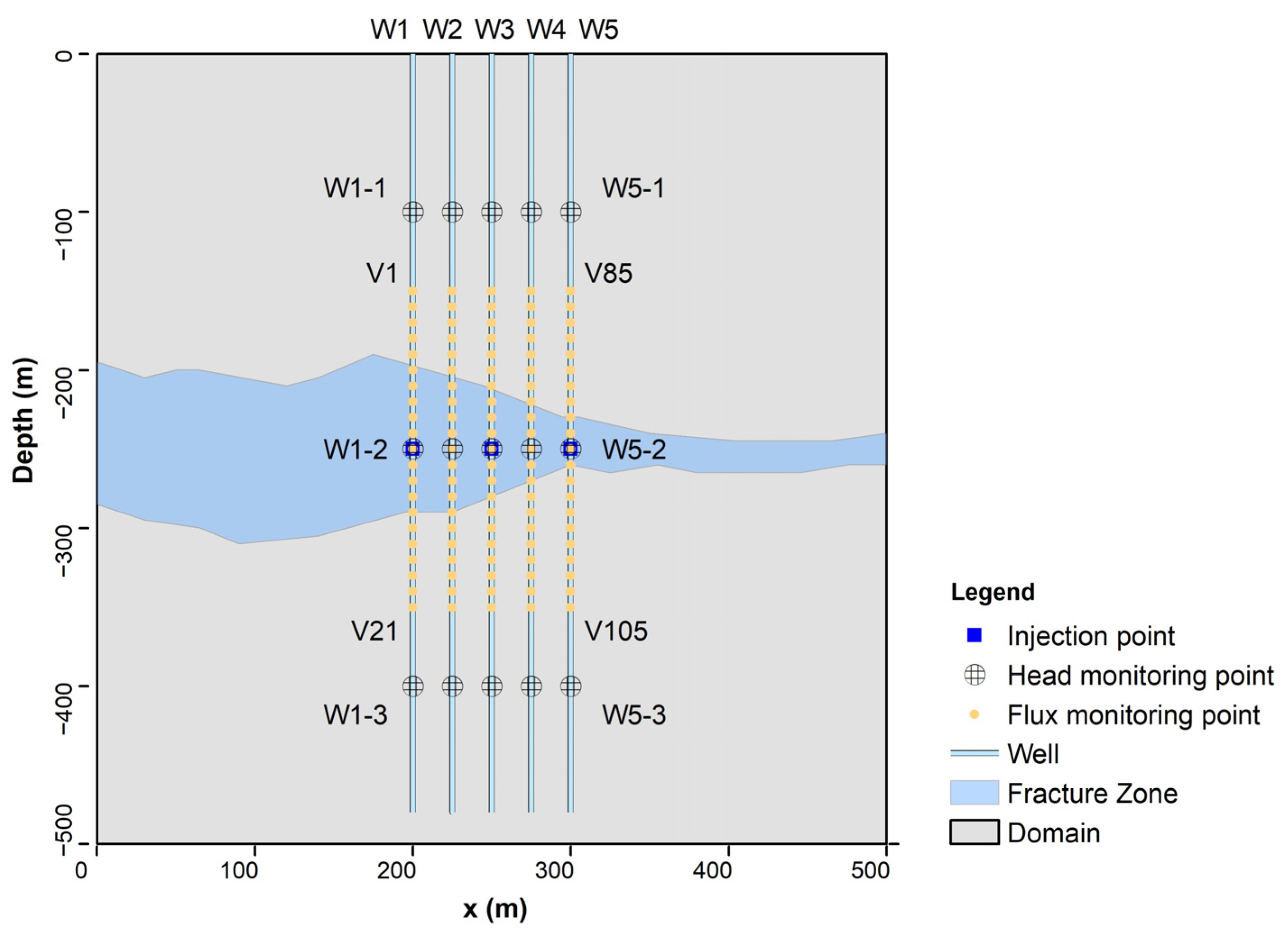
2.1. Synthetical Model

2.1.1. Model Setup

A cross-sectional model of a fractured zone was established as a reference model using the software COMSOL Multiphysics. Synthetic injection tests were conducted to obtain water head and flux datasets. The model is conceptualized as a two-dimensional vertical cross-section of a specific site, with a depth of 500 m and a focused width of 100 m (Figure 1). To avoid boundary condition effects, the model extent is expanded to 500 m by 500 m. A horizontally oriented, irregularly shaped fractured zone passes through the model.

Five monitoring boreholes (Well1–Well5) are placed within the X = 200 m to 300 m range, each spaced 25 m apart. All five boreholes penetrate the fractured zone. Due to the high cost of double-packer observation equipment, multiple water monitoring layers are limited in practice. Thus, each borehole has three water head monitoring locations at y = −100 m, −250 m, and −400 m, totaling 15 head monitoring locations. As mentioned in the introduction, A-DTS provides high-precision distributed flux data, allowing for the continuous monitoring of boreholes. Therefore, the spatial resolution of distributed flux profile data is set to 10 m, with 21 points distributed along each borehole profile in the model.

The boundaries of the reference model are set as constant water head boundaries on the sides, while the top and bottom boundaries are zero-flux boundaries. There is a background groundwater flow from the left side (x = 0 m) to the right side (x = 500 m), with a hydraulic gradient of 0.01. The hydraulic conductance in the fractured zone and matrix is 5 × 10⁻⁴ m/s and 5 × 10⁻⁹ m/s, respectively.

2.1.2. Synthetic Injection Tests Used for Inversion and Validation

To obtain the water head and flux data required for joint inversion, three synthetic injection tests were conducted in the reference model. For each injection test, an injection point was set (specific injection points are shown in

Table 1. Details of synthetic injection tests in reference models with fault zone.

Test ID	Injection Point	Head Dataset	Flux Dataset
Injection-1	Well3-2	H (m)	Vx	Vy
Injection-2	Well1-2	n = 15 × 3	n = 105 × 3	n = 105 × 3
Injection-3	Well5-2

H is the water head; V_x is the horizontal flow rate; V_y is the vertical flow rate; n is the number of data.

), with an injection rate of 10 kg/s (corresponding to a volumetric flow rate of 0.01 m³/s), and the injection duration was 10 days. From each injection test, water head response data from 15 monitoring points across 5 borehole profiles (including the injection point) and distributed flux profiles were obtained.

To obtain the necessary water head and flux data for joint inversion, we conducted three synthetic injection tests within the reference model. In each test, a single injection point was established (specific locations are detailed in Table 1), with a water injection rate of 10 kg/s (equivalent to a volumetric flow rate of 0.01 m³/s) over a period of 10 days.

Table 1 summarizes the synthetic injection tests conducted within the fracture zone reference model, specifying the injection points and the corresponding water head and flux datasets obtained. All data were collected at the end of the injection tests, ensuring that water levels and flow rates at the monitoring points had reached a quasi-steady state. The hydraulic monitoring points provided water head (H) data, while the flux monitoring points provided horizontal and vertical groundwater flow velocities (V_x and V_y, respectively). These datasets served as input sources for the hydraulic tomography inversion to identify fracture permeability characteristics.

Independent hydraulic tests in both the reference model and the estimated permeability distribution fields obtained from the inversion used different injection points from those in the inversion simulations to obtain water level (H) and flow rate (V_x and V_y) distributions for each test. Considering that the actual monitoring simulation range of the reference model is only 100 m × 500 m (expanded to 500 m × 500 m to avoid boundary condition effects), only the area of x = 150 m to 350 m and y = −500 m to 0 m is selected as the validation range (200 m × 500 m). The validation range is divided into a 5 m × 5 m grid (consistent with the VSAFT2 inversion model grid size), and the water levels and flow rates at each grid node (totaling 10,201 validation points) are compared and analyzed using validation scatter plots.

Independent hydraulic tests were conducted within both the reference model and the model with the estimated permeability fields derived from the inversion. These tests used different injection points at Well2-2 (inside the fractured zone), Well3-1 (in the matrix above the fractured zone), and Well4-3 (in the matrix beneath the fractured zone), which are different from those in the inversion simulations to obtain water head and flow. Considering that the monitoring range of the reference model is 100 m × 500 m, validation was limited to x = 150 m to 350 m and y = −500 m to 0 m, covering an area of 200 m × 500 m.

Groundwater head and flux in the validation area, 10,201 validation points in total, were compared and analyzed. The performance was assessed using three indicators: the coefficient of determination (R²), the mean absolute error (MAE), and the root mean square error (RMSE).

2.2. Hydraulic Tomography of Synthetic Head and Flux Data

2.2.1. Inverse Modeling Approach

Hydraulic tomography of the synthetic injection test data from the reference model was conducted using the simultaneous successive linear estimator (SimSLE) algorithm [5]. The SimSLE can estimate the K and S_S distributions as well as their uncertainties by evaluating all the available pumping/injection test data simultaneously. A brief description of the SimSLE is provided below.

In the SimSLE, the hydraulic parameters of the spatial random field are generalized as the following expressions:

$$\left\{\begin{array}{l}\ln K=E\left[\ln K\right]+f\\ \ln S_S=E\left[\ln S_S\right]+s\end{array}\right.$$

(1)

In the above expressions, ln is the natural logarithm, E[ln K] and E[ln S_S] are the mean values, and f and S are the perturbations of the natural logarithm values of the parameters. The instantaneous dynamic water head response caused by the pumping test can be expressed as the sum of the mean value and the perturbation, as follows:

$$H=\overline{H}+h.$$

(2)

The SimSLE method requires starting calculations based on the prior values of the parameter field. The difference between the simulated and the observed water head at sampling points is used for the inversion of hydraulic parameter values in the next iteration. The parameter estimation field is iteratively generated as follows:

$${\widehat{r}}_c^{\left(r+1\right)}={\widehat{r}}_c^{\left(r\right)}+{\omega }^{\mathrm{T}}\left(d^{*}-d^{\left(r\right)}\right).$$

(3)

In the equation, ${\widehat{r}}_c^{\left(r\right)}$ is the parameter estimation value at the r iteration, and the subscript c represents specific conditions. The weight factor ω varies according to the difference between the observed and simulated values at each time node in each observation well. The superscript T represents the transpose matrix, $d^{*}$ is the vector of observed water head, and $d^{\left(r\right)}$ is the water head value calculated by the forward simulation at the r iteration. The weight factor ω, as an important calculation parameter, can be calculated by the following formula:

$$\left[{\epsilon }_{dd}^{\left(r\right)}+{\theta }^{\left(r\right)}\mathrm{diag}\left({\epsilon }_{dd}^{\left(r\right)}\right)\right]{\omega }^{\left(r\right)}={\epsilon }_{dy}^{\left(r\right)}.$$

(4)

In the above formula, ${\epsilon }_{dd}^r$ is the conditional covariance matrix between the secondary datasets (i.e., head, flux magnitude, or flux vector) at the r iteration, and ${\epsilon }_{dy}^r$ is the cross-covariance matrix of the secondary datasets and calculation parameters at the r iteration. θ is the stability coefficient, which needs to be added to the diagonal matrix (${\epsilon }_{dd}^r$) in the calculation to ensure the stability of the solving process. The covariance matrix ${\epsilon }_{dd}^r$ and the cross-covariance matrix ${\epsilon }_{dy}^r$ can be calculated by first-order approximation numerical methods [8] and can be written as follows:

$$\left\{\begin{array}{l}{\epsilon }_{dd}^{\left(r\right)}=J_d^{\left(r\right)}{\epsilon }_{yy}^{\left(r\right)}{J}_d^{\left(r\right)\mathrm{T}}\\ {\epsilon }_{dy}^{\left(r\right)}=J_d^{\left(r\right)}{\epsilon }_{yy}^{\left(r\right)}\end{array}\right.$$

(5)

In the equation, J_d is the sensitivity matrix of the water head to the estimated parameter values. In the first iteration (i.e., r = 0), the covariance matrix ε_yy is composed of prior geological information, such as K and Ss. When the number of iterations is r ≥ 1, the conditional covariance matrix can be calculated by the following formula:

$${\epsilon }_{yy}^{\left(r\right)}={\epsilon }_{yy}^{\left(r-1\right)}-{\omega }^{\mathrm{T}}{\epsilon }_{dy}^{\left(r-1\right)}.$$

(6)

2.2.2. Inverse Model Setup

This study employs VSAFT2 (see https://tian.hwr.arizona.edu/downloads accessed on 10 June 2023) as the numerical code for the inversion model. A vertical profile inversion model is established in VSAFT2, maintaining consistency with the reference model i terms of the range, number, and locations of the water head and flux monitoring points. Given that the input dataset, water heads, and flux at the end of the simulated injection tests represents steady-state flow data, the selected inversion method is a steady-state flow inversion.

To evaluate the impact of different data types (head and flux) on the inversion, three different input datasets were used for hydraulic tomography:

• Model_V uses only the flux dataset, utilizing data from all 105 flux monitoring points;
• Model_H uses only the water head dataset, incorporating data from 15 monitoring points;
• Model_H-V combines the water head and flux data using the results of Model_V as the prior parameter field and then integrating the water head data for joint inversion.

3. Results

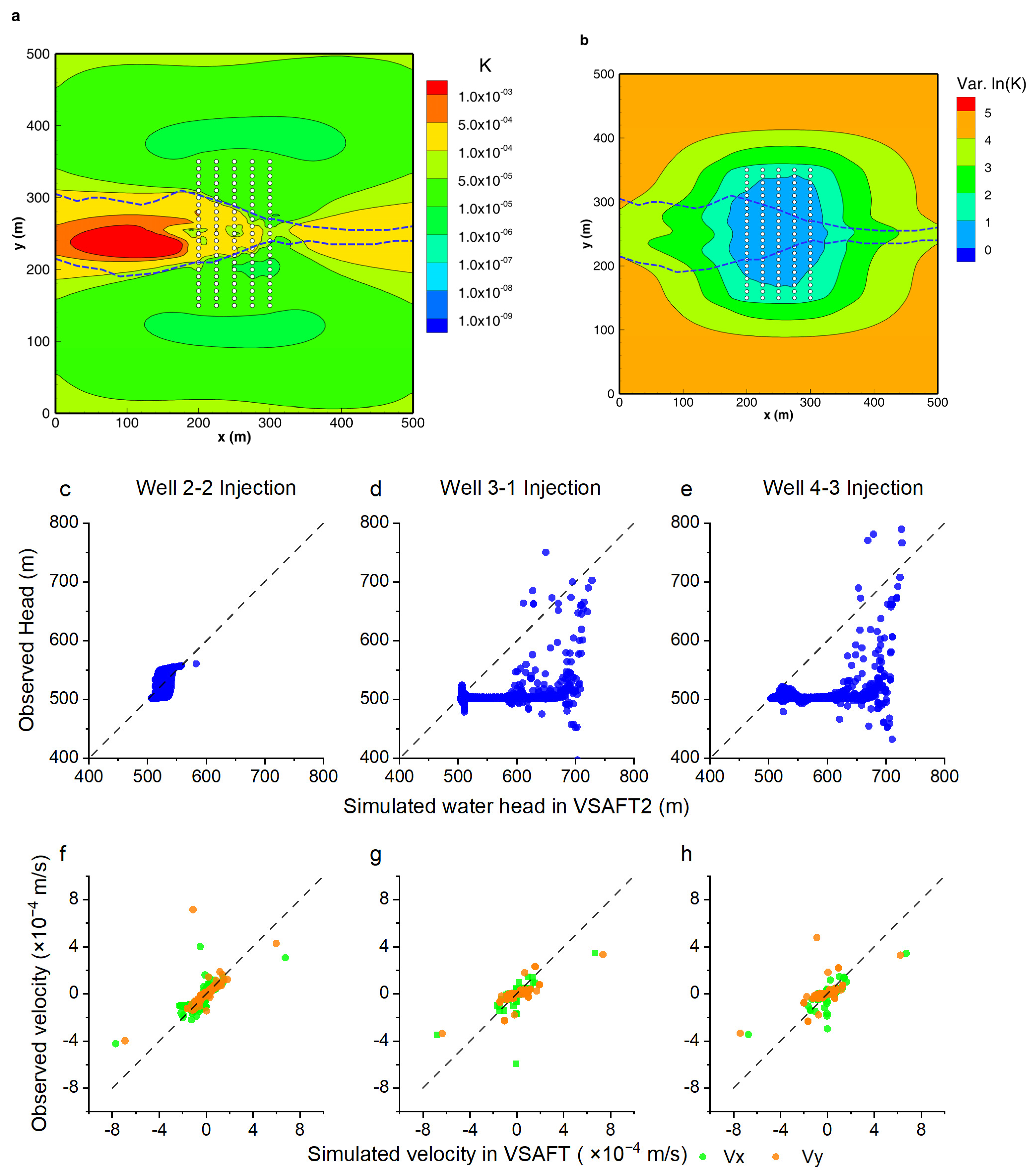
3.1. K Estimates from Flux Data and Model Validation

Figure 2 shows the inversion results of Model_V, based solely on the flux data. By comparing Figure 2a with Figure 1, it can be seen that the permeability distribution estimated from the flux data can largely depict the position of the high-permeability fractured zone. It also accurately reflects the significant morphological change, narrowing the width of the fractured zone at x = 275 m. However, the estimation of matrix permeability in Figure 2a is poor, with the matrix permeability differing significantly from that in the reference model by about three orders of magnitude. The errors in Figure 2a correspond to the uncertainty distribution shown in Figure 2b. The uncertainty is low at the positions where flux information was obtained in the boreholes, while the uncertainty is high in the surrounding matrix areas due to the lack of information.

To validate the performance of the K distribution obtained from the inversion, three new injection wells were activated in both the inverted K field and the reference model, as described in Section 2.1.2. The injection well locations and injection rate in the models are the same. The water head (H) and flow flux (V_x and V_y) distributions for each injection test were obtained. The water heads and flow flux of a total of 10,201 validation points within the validation area were analyzed.

As shown in Figure 2c–e for Model_V, based solely on the 15 water heads monitoring data, water head H fits better for the injection test conducted at the monitoring point located in the high-permeability fractured zone (Well2-2) compared to the injection tests conducted in the matrix (the injection points at Well3-1 or Well4-3), with R² = 0.42892, MAE = 12.3 m, and RMSE = 13.9 m in

Table 2. Validation results for Model_V.

Item	Injection Point	Performance
		MAE	RMSE	R2
H Vx Vy	Well2-2	12.3	13.9	0.42892
		5.25 × 10−6	1.72 × 10−5	0.68148
		2.89 × 10−6	1.52 × 10−5	0.41830
H	Well3-1	923	12,000	0.23953
Vx		1.00 × 10−5	2.00 × 10−5	0.24664
Vy		9.05 × 10−6	1.82 × 10−5	0.42225
H	Well4-3	926	12,000	0.22680
Vx		9.91 × 10−6	1.85 × 10−5	0.35522
Vy		8.28 × 10−6	1.92 × 10−5	0.27644

. When conducting injection validation tests in the matrix, the model tends to underestimate the water level H at the monitoring points, with R² only 0.23953 and 0.22680, respectively.

However, in the validation scatter plots for horizontal flux (V_x) and vertical flux (V_y) (Figure 2f–h), similar differences are not observed—the flux fits well for the injection tests in the high-permeability fracture zone (Well2-2) and the matrix (Well3-1 or Well4-3).

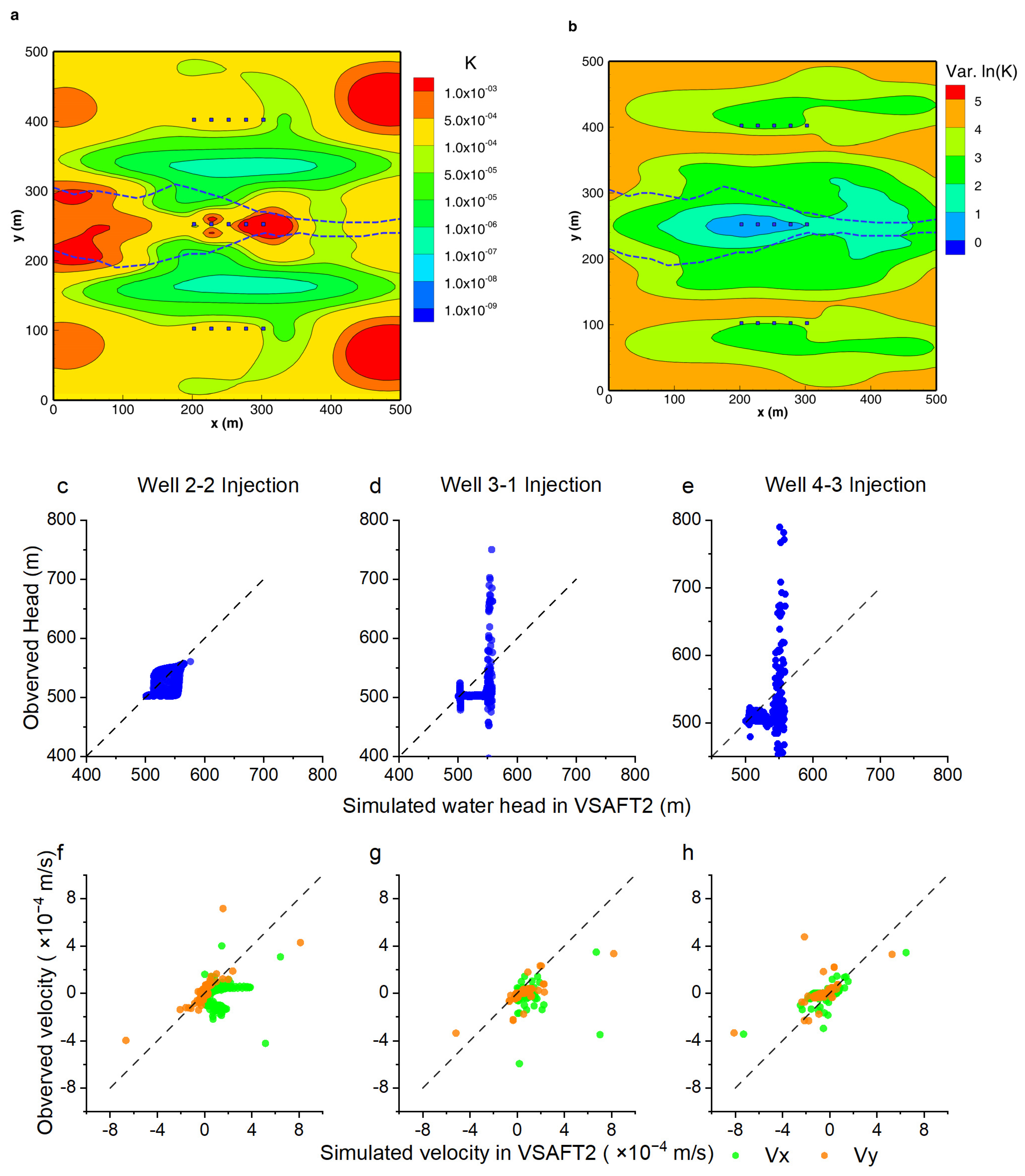
3.2. K Estimates from the Head Data and Model Validation

Figure 3 shows the inversion results of Model_H based on the dataset of 15 water head monitoring points. In Figure 3a, the distribution of the high permeability fractured zone aligns well with the reference model in general, but the fractured zone’s shape shows significant local differences. Particularly at x = 275 m, the fractured zone in the reference model narrows significantly, while in the inversion result, the fractured zone broadens instead.

Additionally, although the inversion results depict the matrix on both sides of the fracture zone as low-permeability areas, the extent of these low-permeability areas is limited in the area where the observation wells are located, which does not match well with the reference model. This error corresponds to the uncertainty distribution shown in Figure 3b. Due to the lack of water head monitoring data, there are high-uncertainty regions around the upper/lower five monitoring points, indicating a significant error in depicting the low-permeability regions of the matrix.

As shown in Figure 3c–e for Model_H, based solely on the 15 water head monitoring datasets, water head H fits better for the injection test conducted at the monitoring point located in the high-permeability fractured zone (Well2-2) compared to the injection tests conducted in the matrix (injection points at Well3-1 or Well4-3), with R² = 0.38611, MAE = 9.28 m, and RMSE = 17.8 m in

Table 3. Validation results for Model_H.

Item	Injection Point	Performance
		MAE	RMSE	R2
H Vx Vy	Well2-2	9.28	17.8	0.38611
		1.54 × 10−5	4.90 × 10−5	0.00719
		3.06 × 10−6	1.37 × 10−5	0.52576
H	Well3-1	901	12,100	0.03772
Vx		1.10 × 10−5	3.11 × 10−5	0.00133
Vy		4.12 × 10−6	1.54 × 10−5	0.46020
H	Well4-3	903	12,100	0.04587
Vx		1.03 × 10−5	2.33 × 10−5	0.30368
Vy		4.24 × 10−6	1.85 × 10−5	0.23828

. When conducting injection validation tests in the matrix, the model tends to underestimate water level H at the monitoring points, with R² only 0.03772 and 0.04587, respectively.

However, in the validation scatter plots for horizontal flux (V_x) and vertical flux (V_y) (Figure 3f–h), similar differences are not observed—the flux fits well for the injection tests in the high-permeability fracture zone (Well2-2) and the matrix (Well3-1 or Well4-3).

3.3. K Estimates from Head–Flux Data and Model Validation

Figure 4a,b show the results of Model_V-H, combining the head data with the flux data. In Figure 4a, it can be seen that the addition of the flux data improves the depiction of the high-permeability fractured zone’s shape and distribution, as well as the characterization of the matrix on both sides of the fractured zone. Especially for the characterization of the matrix on both sides, the flux information within the y = 100~400 m region reduces the uncertainty of the inversion results in this range (Figure 4b), making the distribution of low-permeability areas on both sides in Figure 4a more reasonable.

Figure 4c also shows results similar to Model_H, which used only the water heads in the inversion. The injection test conducted at the monitoring point located in the high-permeability fractured zone (Well2-2) fits water head H better with R² = 0.30778 than the injection tests conducted at the matrix monitoring points with R² = 0.14469 and 0.18428, respectively. There was no significant difference in the goodness of fit of the flux in the validation of the different injection tests. However, comparing the performance in Table 3 and

Table 4. Validation results for Model_H.

Item	Injection Point	Performance
		MAE	RMSE	R2
H Vx Vy	Well2-2	13.5	21.8	0.30778
		9.69 × 10−6	4.04 × 10−5	0.33187
		3.05 × 10−6	2.30 × 10−5	0.10038
H	Well3-1	925	12,000	0.14469
Vx		1.04 × 10−5	2.62 × 10−5	0.15412
Vy		6.08 × 10−6	2.35 × 10−5	0.31949
H	Well4-3	926	12,000	0.18428
Vx		9.74 × 10−6	2.38 × 10−5	0.23306
Vy		6.04 × 10−6	2.68 × 10−5	0.12498

with H-K and H-V-K shows that the addition of the flux data improves the validation of H, especially in the injection tests in the matrix zone (Well3-1 and Well4-3).

4. Discussion

4.1. Differences between Head Data and Flux Data in K Estimation and Fractured Zones Characterization

This section will compare the inversion results using only water head data (Model_H, See Figure 3) and those using only the flux rate dataset (Model_V, See Figure 2), analyzing the impact of different data types on the inversion and on the identification and characterization of the high permeability fractured zone.

Figure 2a, which uses only the flux data in inversion, more accurately depicts the shape of the high-permeability fractured zone and also provides a more reasonable distribution of the low-permeability regions of the surrounding low-permeability bedrock. Additionally, the independent injection validation results for Model_V are generally better than for Model_H, especially in terms of the flux validation point (see Table 2 and Table 3).

Although the inversion using flux data better characterizes the fractured zone distribution, the permeability value difference between the high-permeability region (K approximately 5 × 10⁻³ m/s) and the low-permeability region (K approximately 5 × 10⁻⁶ m/s) in the inversion results is only about three orders of magnitude, which fails to reflect the approximately five orders of magnitude permeability difference of those in the reference model. Although the estimated K is similar in the high-permeability zone, the estimated K of Model_H in the low-permeability region (~1.00 × 10⁻⁷ m/s) is closer to that in the reference field; thus, it better reflects the significant permeability differences in the reference field.

Therefore, in the inversion of K to identify high-permeability fractured zones, the inversion model using only the flux data performs better overall in characterizing the fracture shape, but it is slightly worse in depicting specific K values.

It should be noted that in the above discussion, the number of flux monitoring points is greater than the number of water head monitoring points, which is probably the case in a real site. The increase in the number of monitoring points means that the information-gathering area is enlarged. The densely distributed flux monitoring points near the fractured zone enables the inversion model to reflect the distribution of the fractured zone more reasonably and accurately, thereby significantly enhancing the identification and characterization of the fractured zone. However, even if the number of flux monitoring points is several times that of the water head monitoring points, the inversion model’s reliance solely on flux data does not necessarily guarantee more accurate permeability values compared to the inversion model’s reliance solely on water head data.

4.2. Enhancements in Hydraulic Tomography through Flux Data Integration

The permeability distribution inverted from the data of 15 water head monitoring points (Model_H) generally reflects the position of the fractured zone (Figure 3a). Additionally, due to the limitation of the water head monitoring point, there are some errors in depicting the distribution of the low-permeability matrix. In Figure 5, when the number of water head monitoring points is reduced to five (Model_5H, see Supplementary Materials Section S1, Figure S1) or three (Model_3H, see Supplementary Materials Section S2, Figure S4), the inverted permeability distribution can still generally describe the position of the fractured zone, but there are significant errors in describing the whole. This indicates that when the input data is only water heads, the inverted permeability distribution is hard to depict in the fractured zone.

This indicates that when the number of water head monitoring points is small, the inverted permeability distribution lacks sufficient information to constrain the iterative results, leading to non-uniqueness in the inversion results. The inversion results do not actually reflect the true permeability distribution.

The introduction of flux data has a significant positive impact on the HT inversion results. As shown in Figure 3a, Figure 4a and Figure 5, after introducing the vertically distributed flux data for joint inversion, the permeability distribution (Model_H-V, Model_5H-V, and Model_3H-V) is significantly improved, better depicting the position, the shape of the fractured zone, and the surrounding low-permeability bedrock. Even when compared to Model_H, which can roughly depict the position and distribution of the fractured zone, the introduction of flux data optimizes the inversion K distribution, the depiction of the fracture zone’s shape, and the surrounding matrix distribution. Especially when the number of water head monitoring points is gradually reduced to five and three, the improvement in depicting the fracture shape with the flux data is more significant.

The above results indicate that introducing distributed flux data for joint inversion can effectively enhance the ability of the HT inversion method to identify and characterize the fractured zone. Previous research on the joint inversion of water head and flux data [20] shows that flux and water head data at the same monitoring point cannot be substituted for one another. Even with identical numbers and locations of monitoring points, HT inversion results using only flux data differ from those using only water head data. This indicates that flux data contains unique, non-redundant information.

This study confirms that the non-redundant information inherent in flux data plays an active role in the HT inversion process, particularly in characterizing the permeability structure. Because flux is vector data, it includes not only specific flux values but also flow directions. Velocity data is more sensitive to relative differences in permeability compared to specific permeability values, which enhances the depiction of permeability distribution. However, this characteristic also leads to poorer performance in estimating absolute permeability values.

4.3. Application Strategy of Head and Flux Data in Fractured Zone Characterization Using Hydraulic Tomography

Increasing the number of monitoring points is crucial for improving the results of the joint inversion of water head and flux data. The improvement due to increased monitoring points is more significant in joint inversion compared to using a single data type [20]. However, deciding whether to increase head or flux data is a strategic challenge in the practical application of joint inversion to characterize fractured zones. According to the inversion model results, using data from 15 water head monitoring points can achieve a reasonably accurate permeability distribution (Model_H). However, this high spatial resolution, with five adjacent boreholes each containing three multilevel water head monitoring points, is costly and uncommon in actual field sites.

Therefore, considering the cost of the double-packer multi-level monitoring system for deep boreholes in bedrock, a scheme with fewer water head monitoring points, such as Model_5H or Model_3H, combined with a significant increase in vertically distributed flux monitoring points, would be more beneficial for practical field applications. Vertically distributed flux data can effectively constrain the non-uniqueness of the inversion model and accurately characterize the site’s permeability structure. Additionally, the cost of obtaining flux data using the active DTS method is relatively low: the cost of one multi-level monitoring system in a single deep borehole could support the active DTS testing of all the wells at a site, making it advantageous for the practical application of the joint inversion method.

Considering that different types of monitoring data may vary in magnitude and dimensions, allocating weights to different types of observation data in joint inversion is also a challenge. Typically, the algorithm assigns equal weight to different types of data during the iteration process. When the magnitudes and dimensions of all observation data types are similar, this approach reflects the information of all data in a balanced manner. However, significant differences in magnitude or dimensions among different data types can result in the information contained in the smaller magnitude data being overshadowed by the larger magnitude data. Generally, the magnitude of flow flux data is often smaller than that of water head data. For instance, in this study’s reference model, the magnitude of the flow flux data, about 10⁻⁴~10⁻⁹ m/s, is much smaller than that of the water head data, which is generally greater than 10². Directly incorporating both flux and head data into the inversion algorithm may lead to permeability estimation being predominantly controlled by the head data and thereby neglecting the flux data.

To solve this problem, the weight matrix in the algorithm can be optimized based on the differences in magnitude and dimensions among the observation datasets. However, considering that dataset differences vary by site, manually optimizing the weight matrix is costly. From a practical application perspective, this study proposes the following strategy for joint inversion methods of water head and flow flux data in fractured rock: First, perform the inversion based on dense flux data to obtain a permeability distribution with structural features as prior information. Then, combine this with limited water head data for joint inversion, optimizing the permeability values and distribution of the fractured zone.

5. Conclusions

This study investigates the potential of using HT joint inversion based on groundwater head and flux data to characterize fractured zones in bedrock, especially considering the impact of cost-induced differences in the quantity of head and flux data in actual field conditions. Synthetic injection tests were conducted in a fractured zone reference model to obtain water head and flux datasets of different quantities. Then, K distribution was estimated by hydraulic tomography, using the SimSLE based on pure water head data, pure flux data, and head–flux joint data. Additionally, validation tests were conducted in both the estimated permeability model and the reference model to obtain water head and flux at each monitoring point in the independent boreholes. By comparing the simulated water heads/flux and the uncertainty distribution of the estimated fields, the impact of different input data on the identification of fracture zone permeability was discussed.

By comparing inversion results with different sets of head data, flux data, and a combination of the two, it can be seen that the joint inversion of head and flux data can effectively enhance HT’s accuracy in identifying the permeability characteristics of fractured zones. Especially when water head data is limited, which is often the case in actual conditions, flux information can significantly improve the identification and characterization of the permeability distribution. This is not only because the flux data itself brings non-redundant information but also because an increase in the number of monitoring points reduces the uncertainty of the inversion results.

Considering that the rapid development of active DTS method could provide high-resolution spatial and temporal data on groundwater flux at relatively low cost, from the perspective of the practical application of HT in the characterization of fractured zones, it is better to estimate the permeability distribution base on the flux data, use it as prior information in further inversions, and combine them with limited water head data to optimize the permeability distribution. The findings of this study provide a promising method for determining the permeability distribution in real fractured rock sites and offer a relatively low-cost and efficient application strategy for detecting and characterizing fractured zones.

References

1. Deng, H.; Spycher, N. Modeling Reactive Transport Processes in Fractures. Rev. Mineral. Geochem. 2019, 85, 49–74. [Google Scholar] [CrossRef]
2. Maréchal, J.C.; Dewandel, B.; Subrahmanyam, K. Use of hydraulic tests at different scales to characterize fracture network properties in the weathered-fractured layer of a hard rock aquifer. Water Resour. Res. 2004, 40, W11508. [Google Scholar] [CrossRef]
3. Ren, S.; Gragg, S.; Zhang, Y.; Carr, B.J.; Yao, G. Borehole characterization of hydraulic properties and groundwater flow in a crystalline fractured aquifer of a headwater mountain watershed, Laramie Range, Wyoming. J. Hydrol. 2018, 561, 780–795. [Google Scholar] [CrossRef]
4. Cardiff, M.; Barrash, W. 3-D transient hydraulic tomography in unconfined aquifers with fast drainage response. Water Resour. Res. 2011, 47, W12518. [Google Scholar] [CrossRef]
5. Xiang, J.; Yeh, T.-C.J.; Lee, C.-H.; Hsu, K.-C.; Wen, J.-C. A simultaneous successive linear estimator and a guide for hydraulic tomography analysis. Water Resour. Res. 2009, 45, W02432. [Google Scholar] [CrossRef]
6. Zhu, J.; Yeh, T.-C.J. Characterization of aquifer heterogeneity using transient hydraulic tomography. Water Resour. Res. 2005, 41, W07028. [Google Scholar] [CrossRef]
7. Yeh, T.-C.J.; Liu, S. Hydraulic tomography: Development of a new aquifer test method. Water Resour. Res. 2000, 36, 2095–2105. [Google Scholar] [CrossRef]
8. Zha, Y.; Yeh, T.-C.J.; Illman, W.A.; Tanaka, T.; Bruines, P.; Onoe, H.; Saegusa, H. What does hydraulic tomography tell us about fractured geological media? A field study and synthetic experiments. J. Hydrol. 2015, 531, 17–30. [Google Scholar] [CrossRef]
9. Illman, W.A. Hydraulic Tomography Offers Improved Imaging of Heterogeneity in Fractured Rocks. Groundwater 2014, 52, 659–684. [Google Scholar] [CrossRef]
10. Illman, W.A.; Liu, X.; Takeuchi, S.; Yeh, T.-C.J.; Ando, K.; Saegusa, H. Hydraulic tomography in fractured granite: Mizunami Underground Research site, Japan. Water Resour. Res. 2009, 45, W01406. [Google Scholar] [CrossRef]
11. Zha, Y.; Yeh, T.-C.J.; Illman, W.A.; Tanaka, T.; Bruines, P.; Onoe, H.; Saegusa, H.; Mao, D.; Takeuchi, S.; Wen, J.-C. An Application of Hydraulic Tomography to a Large-Scale Fractured Granite Site, Mizunami, Japan. Groundwater 2016, 54, 793–804. [Google Scholar] [CrossRef] [PubMed]
12. Hao, Y.; Yeh, T.-C.J.; Xiang, J.; Illman, W.A.; Ando, K.; Hsu, K.-C.; Lee, C.-H. Hydraulic Tomography for Detecting Fracture Zone Connectivity. Groundwater 2008, 46, 183–192. [Google Scholar] [CrossRef] [PubMed]
13. Sharmeen, R.; Illman, W.A.; Berg, S.J.; Yeh, T.-C.J.; Park, Y.-J.; Sudicky, E.A.; Ando, K. Transient hydraulic tomography in a fractured dolostone: Laboratory rock block experiments. Water Resour. Res. 2012, 48, W10532. [Google Scholar] [CrossRef]
14. Sreeparvathy, V.; Kambhammettu, B.V.N.P.; Peddinti, S.R.; Sarada, P.S.L. Application of ERT, Saline Tracer and Numerical Studies to Delineate Preferential Paths in Fractured Granites. Groundwater 2019, 57, 126–139. [Google Scholar] [CrossRef]
15. Ringel, L.M.; Illman, W.A.; Bayer, P. Recent developments, challenges, and future research directions in tomographic characterization of fractured aquifers. J. Hydrol. 2024, 631, 130709. [Google Scholar] [CrossRef]
16. Tiedeman, C.R.; Barrash, W. Hydraulic Tomography: 3D Hydraulic Conductivity, Fracture Network, and Connectivity in Mudstone. Groundwater 2020, 58, 238–257. [Google Scholar] [CrossRef]
17. Dong, Y.; Fu, Y.; Yeh, T.-C.J.; Wang, Y.-L.; Zha, Y.; Wang, L.; Hao, Y. Equivalence of Discrete Fracture Network and Porous Media Models by Hydraulic Tomography. Water Resour. Res. 2019, 55, 3234–3247. [Google Scholar] [CrossRef]
18. Pouladi, B.; Bour, O.; Longuevergne, L.; de La Bernardie, J.; Simon, N. Modelling borehole flows from Distributed Temperature Sensing data to monitor groundwater dynamics in fractured media. J. Hydrol. 2021, 598, 126450. [Google Scholar] [CrossRef]
19. Michael Tso, C.-H.; Zha, Y.; Jim Yeh, T.-C.; Wen, J.-C. The relative importance of head, flux, and prior information in hydraulic tomography analysis. Water Resour. Res. 2016, 52, 3–20. [Google Scholar] [CrossRef]
20. Zha, Y.; Yeh, T.-C.J.; Mao, D.; Yang, J.; Lu, W. Usefulness of flux measurements during hydraulic tomographic survey for mapping hydraulic conductivity distribution in a fractured medium. Adv. Water Resour. 2014, 71, 162–176. [Google Scholar] [CrossRef]
21. Liu, F.; Yeh, T.-C.J.; Song, X.; Wang, Y.-L.; Wen, J.-C.; Hao, Y.; Wang, W. Temporal sampling and role of flux measurements for subsurface heterogeneous characterization in groundwater basins using hydraulic tomography. Hydrol. Process. 2021, 35, e14299. [Google Scholar] [CrossRef]
22. Simon, N.; Bour, O.; Lavenant, N.; Porel, G.; Nauleau, B.; Klepikova, M. Monitoring groundwater fluxes variations through active-DTS measurements. J. Hydrol. 2023, 622, 129755. [Google Scholar] [CrossRef]
23. Simon, N.; Bour, O. An ADTS Toolbox for Automatically Interpreting Active Distributed Temperature Sensing Measurements. Groundwater 2023, 61, 215–223. [Google Scholar] [CrossRef] [PubMed]
24. Munn, J.D.; Maldaner, C.H.; Coleman, T.I.; Parker, B.L. Measuring Fracture Flow Changes in a Bedrock Aquifer Due to Open Hole and Pumped Conditions Using Active Distributed Temperature Sensing. Water Resour. Res. 2020, 56, e2020WR027229. [Google Scholar] [CrossRef]
25. Simon, N.; Bour, O.; Lavenant, N.; Porel, G.; Nauleau, B.; Pouladi, B.; Longuevergne, L.; Crave, A. Numerical and Experimental Validation of the Applicability of Active-DTS Experiments to Estimate Thermal Conductivity and Groundwater Flux in Porous Media. Water Resour. Res. 2021, 57, e2020WR028078. [Google Scholar] [CrossRef]
Figure 1. Vertical cross-section of the reference model and locations of head monitoring points and velocity monitoring points in the model; K = 5 × 10⁻⁴ m/s is in the blue fracture area, and K = 5 × 10⁻⁹ m/s is in the other area.
Hydrology 11 00122 g001
Figure 2. Inversion results of Model_V and its validation. (a) is the inversion result based on the flux dataset; (b) is the uncertainty distribution with white circles indicating flux monitoring points; (ch) are head and flux validation.
Hydrology 11 00122 g002
Figure 3. Inversion results for Model_H and its validation. (a) is the inversion result based on the head dataset; (b) is the uncertainty distribution with blue squares indicating water head monitoring points; (ch) are validation scatter plots.
Hydrology 11 00122 g003
Figure 4. Inversion results of Model_H-V and its validation. (a) is the inversion result combining head and flux data; (b) shows the uncertainty distribution of the inversion results, with white circles indicating the input head monitoring points and black dots indicate the flux monitoring points; (ch) are the validation scatter plots.
Hydrology 11 00122 g004
Figure 5. Comparison of inversion K fields using a different number of water head points. (a) is the inversion result based on 5 head monitoring points (Model_5H); (b) is the inversion result based on 5 head monitoring points and flux data (Model_5H_V); (c) is the inversion result based on 3 head monitoring points (Model_3H); (d) is the inversion result based on 3 head monitoring points and flux data (Model_3H_V). Blue squares indicate water head monitoring points and white circles indicate flux monitoring points.
Hydrology 11 00122 g005