Statistical Model Development for Estimating Soil Hydraulic Conductivity Through On-Site Investigations

Abstract

In arid regions, irrigated agriculture is mainly dependent on groundwater. In Pakistan, 73% of agricultural land is directly or indirectly irrigated through groundwater. In Punjab (Pakistan), 1.2 million private tube wells are operating, mainly extracting 90% of the country’s groundwater. Most of these wells are poorly designed due to improper site investigations and poor estimations of the aquifer’s hydraulic parameters. As a result, most wells become dry, causing considerable financial losses to farmers. Hence, optimizing the well-designed parameters through proper soil investigations is essential. This research aims to develop a statistical model for estimating the hydraulic conductivity of soil through on-site investigation: five sites were selected in Multan (Pakistan), and seven samples were collected at each location from 3, 6, 9,12,15,18, and 21 m depth. For hydraulic conductivity, soil texture, and porosity, soil laboratory tests were carried out. Finally, a statistical model was developed using hydrological parameters such as average grain size distribution (D₅₀), uniformity coefficient (U), and porosity (n). Statistically computed hydraulic conductivity was verified with experimentally measured and empirically derived hydraulic conductivity. Statistically measured hydraulic conductivity showed closer agreement with experimentally measured hydraulic conductivity than the empirically measured hydraulic conductivity: root mean square error (RMSE), correlation coefficient (Cc), and mean absolute error (MAE) are, respectively, equal to 0.013, 0.93, and 0.011.

1. Introduction

Soil is generally considered as an important medium in many disciplines of engineering and natural science [1]. Different research studies highlight its importance, e.g., ref. [2] discusses its importance in the foundation engineering and also identifies it as suitable medium for agricultural development. Various soil characteristics such as structure, texture, and hydrological properties are considered important in irrigated agriculture, tube well design, and drainage design. Hydraulic conductivity is an important hydraulic property of soil that delineates flow through porous media and is essential for groundwater research and management strategies [3]. Its proper investigation is crucial to research seepage in earth dams and levees and perform stability evaluations of earth structures under seepage pressures [4]. Similarly, in terms of irrigation system design, saturated hydraulic conductivity determination is necessary to understand water movement in saturated and unsaturated zones to learn the water holding capacity of soil [5].

The various characteristics of porous media, such as porosity, structural orientation, and fluid properties, affect soil hydraulic conductivity [6]. The hydraulic conductivity is directly proportional to the size of the grains, which is generally used as a basis for assessing hydraulic conductivity during the initial stages of aquifer investigation. The previous literature discussed various traditional field and laboratory techniques for assessing hydraulic conductivity [7]. However, traditional methods use a limited comprehension of the hydraulic boundaries and aquifer geometry in the field, which sometimes obstructs the precise measurement of hydraulic conductivity. In contrast, laboratory techniques have cost and time limitations [8]. To address these challenges, empirical relationships were developed to compute hydraulic conductivity based on grain size analysis [9]. However, in the absence of an appropriate empirical relation such as grain size, it may lead to the underestimation of hydraulic conductivity [10]. Considering this limitation, [1] indicated that most of these empirical relationships overestimate or underestimate the value of hydraulic conductivity. This study will develop a statistical model for calculating hydraulic conductivity using the soil’s hydrological parameters, which may help in addressing these issues.

Additionally, most of the previous studies on hydraulic conductivity estimation were based on the use of sandy and gravel-packed soil and did not consider clayey soil, except for [11], who performed their investigation on clayey soil. However, ref. [11] used an empirical relationship only for calculating hydraulic conductivity. Their investigation was not based on statistical methods. Therefore, this study will also be innovative in the sense that it also considers clayey soil for developing a statistical model. Therefore, it may be applicable on a wide range of soils for estimating hydraulic conductivity.

Table 1. Literature review of previous studies.

Researcher	Area of Study	Techniques	Conclusion
J. Odong [11]	China	Empirical relationship	Kozeny Carman was the best estimator
A Chandel [1]	India	Empirical relationships, lab methods, and regression analysis	Developed model was the best estimator
J. Song [12]	Nebraska and Elkhorn River	Falling-head permeameter test	Changed C values computed stream bed Kv
J. M. Ishaku [13]	Nigeria	Empirical equations	Terzaghi and K-C formulas were the best estimators
F. Pliakas [14]	Greece	Lab method, empirical relationship	Loudon formula was most accurate
J. Rosas [6]	Four depositional environments at global locations	Lab test and the empirical relationship	Empirical hydraulic conductivity does not correlate with measured values
S. Yoon [15]	South Korea	Regression analysis	Regression model showed R2 = 0.92
M. Naeej [16]	Iran	Lab method and model tree method	Model tree formula provided accurate results
J. Michael [17]	Nigeria	Seven empirical models and constant head method	Kozeny model was the best estimator

provides a review of all previous studies.

Table 1 indicates the importance of hydraulic conductivity determination in different studies. This study examines the role of hydraulic conductivity in terms of groundwater well design. Groundwater provides supplemental irrigation in arid and semi-arid regions of the world [18]. Since 1950, South Asia has seen a significant increase in irrigation intensity, with India, Pakistan, and Bangladesh extracting approximately 320 billion m³ of groundwater annually [19,20]. In the 1960s, there were government-initiated Salinity Control and Reclamation Projects (SCARPs), which caused an increase in groundwater supplies [21,22]. Assured and reliable supplies of groundwater caused an increase in private tube well growth from 30,000 in 1960 to over 1.2 million in 2018, with over 90% being in Punjab [23,24]. However, many wells are poorly designed without considering aquifer hydraulic parameters, leading to premature failures and financial losses for farmers [25]. Over-extraction has depleted aquifers, forcing deeper wells, increasing costs, and raising the risk of aquifer salinization [26,27]. Farmers in Punjab and Sindh face rising irrigation expenses and declining crop yields as wells dry up or become saline, threatening their livelihoods and food security [28,29]. Additionally, inadequate irrigation management has intensified soil salinity, particularly in Sindh, where waterlogging from poor drainage further reduces crop productivity [30]. Optimizing well design through accurate hydraulic conductivity measurement and improved statistical models is necessary to address these challenges.

This study holds significant value for Pakistan’s agricultural sector, which relies heavily on groundwater irrigation. By developing a robust statistical model for measuring hydraulic conductivity using soil parameters like D₅₀, uniformity coefficient, and porosity, this research will enable better sound design, reduce the risk of wells drying prematurely, and minimize financial losses for farmers. The present study aims to develop a statistical model based on sandy and clayey soil for calculating the hydraulic conductivity of borehole soil samples. The model developed herein will provide insight into the most reliable method for predicting hydraulic conductivity, ultimately contributing to more sustainable groundwater usage and improved agricultural productivity in regions like Punjab, where groundwater resources are critical.

The hydraulic conductivity model for sandy soils in borehole screen design can help determine the appropriate screen size and material to ensure adequate water extraction while preventing sand particles from entering the borehole. Moreover, the model can help optimize the design by considering factors such as the flow rate, the size of the sand particles, and the potential for clogging or erosion. By applying the model developed for sandy soil, engineers can ensure that the borehole screen allows for efficient water extraction, maintains a long operational life, and minimizes maintenance costs.

However, the aspect that makes this study more significant is the presence of clayey soil. In drainage filter design, the hydraulic conductivity of clayey soils plays a critical role in managing water flow and preventing clogging. Clayey soils, characterized by fine particles and low permeability, often require precise hydraulic conductivity calculations to ensure that water drains effectively while preventing soil particles from entering the drainage system. The developed model for clayey soils can be applied to select the appropriate filter material and to design the geometry of the filter to maintain a balance between adequate drainage and soil retention. This ensures the filter’s efficacy in water management and safeguards against soil erosion, particularly in areas susceptible to water accumulation or inadequate drainage that may result in structural damage.

2. Materials and Methods

2.1. Study Area

Multan is located in Punjab, Pakistan, along the banks of the Chenab River, at an elevation of 122 m above sea level. Covering an area of approximately 3721 km² in the arid agro-ecological zone of Pakistan, Multan boasts 759,766 acres of cultivated land. The major crops grown in Multan include wheat, cotton, rice, sugarcane, and fodder. Multan is especially renowned for its mangoes, which are known worldwide. Groundwater depths in Multan range from 12 to 15 m. The boring process was carried out at five different locations in Multan, as shown in Figure 1. The borehole was drilled to a depth of approximately 21 m. A total of 35 samples were collected; each sample was collected at 3 m depth [1] and samples were averaged using the method discussed in [31].

2.2. Grain Size Analysis and Porosity Determination

Gathering undisturbed soil samples with constant soil moisture and texture was challenging. Therefore, samples of disturbed soil were gathered. To replicate field conditions, the samples were appropriately repacked in the permeameter to re-establish the original conditions as outlined in [1]. The widely employed method for sieve analysis outlined in [32] was applied to evaluate the particle size of the samples and ascertain their particle size characteristics. However, the sieve analysis was unable to ascertain the complete grain size of five samples due to the clayey composition of these samples. Therefore, a hydrometer analysis was performed using the standard technique outlined in [33] for a thorough grain size distribution. The grain size distribution D₆₀ and D₁₀ were derived from the grain size curve, and the uniformity coefficient was computed using the following formula.

$$U={\displaystyle \frac{D_{60}}{D_{10}}}$$

(1)

U is the uniformity coefficient, whereas D₆₀ and D₁₀ are grain size (mm) at 10% and 60% finer. From the value of uniformity coefficient U for all the samples, the porosity of these samples was calculated by using the formula recommended by [11]:

$$n=0.255\left(1+{0.83}^u\right)$$

(2)

where U is the uniformity coefficient and n is the porosity of soil, and both are dimensionless. However, before calculating porosity, the formula was validated and tested by comparing its computed values with the formula discussed in [32], referred to as the mass densities relationship in terms of void ratio. Porosity was advantageous in calculating hydraulic conductivity through empirical equations, and a relationship was developed between experimentally measured hydraulic conductivity and porosity.

2.3. Estimation of Hydraulic Conductivity Using Laboratory Method and Empirical Relationships

Hydraulic conductivity was measured in the laboratory using two main techniques: falling head and constant head. The soil samples were compacted in the permeameter, and an average value of hydraulic conductivity was taken for each sample using the standard approach as indicated by [34]. Sand and gravelly soil containing coarser particles were treated with a constant head method. However, when the constant head method could not assess the hydraulic conductivity due to finer particles such as silt and clay, the falling head method was utilized [35]. Based on previous literature, nine empirical formulae were identified for calculate hydraulic conductivity. These formulae, along with their descriptions, are provided below

• Hazen [36]

$$K={\displaystyle \frac{g}{v}}\left[1+10\left(n-0.26\right)\right]{D_{10}}^2$$

(3)

where K = hydraulic conductivity cm/s, g = gravitational acceleration (cm/s²), v = kinematic viscosity (cm²/s), β = sorting coefficient = 6 × 10⁻⁴, n = porosity, D₁₀ = effective grain sizes (mm) with 10% passing, U = uniformity coefficient. This formula is applicable when 0.1 mm < D₁₀ < 3 mm, U < 5.

2.

Slichter [37]

$$K={\displaystyle \frac{g}{v}}ßn^{3.287}{D_{10}}^2$$

(4)

where K = hydraulic conductivity cm/s, g = gravitational acceleration (cm/s²), v = kinematic viscosity (cm²/s), β = sorting coefficient = 1 × 10⁻², n = porosity, D₁₀ = effective grain sizes (mm) with 10% passing, U = uniformity coefficient. This formula is applicable when 0.01 mm < D₁₀ < 5 mm.

3.

Terzaghi [38]

$$K={\displaystyle \frac{g}{v}}ß({{\displaystyle \frac{n-0.13}{\sqrt[3]{1-n}}})}^2{D_{10}}^2$$

(5)

where K = hydraulic conductivity cm/s, g = gravitational acceleration (cm/s²), v = kinematic viscosity (cm²/s), β = sorting coefficient = 10.7 × 10⁻³ for smooth grains and 6.1 × 10⁻³ for coarse grains, n = porosity, D₁₀ = effective grain sizes (mm) with 10% passing, U = uniformity coefficient. This formula is applicable for large the grain sand.

4.

Kozeny–Carman [39,40,41]

$$K={\displaystyle \frac{g}{v}}ß\left[{\displaystyle \frac{n^3}{{(1-n)}^2}}\right]{D_{10}}^2$$

(6)

where K = hydraulic conductivity cm/s, g = gravitational acceleration (cm/s²), v = kinematic viscosity (cm²/s), β = sorting coefficient = 8.3 × 10⁻³, n = porosity, D₁₀ = effective grain sizes (mm) with 10% passing, U = uniformity coefficient. This formula is applicable D₁₀ < 3.0 mm suitable for gravel, sand, and silt.

5.

Harleman [42]

$$K={\displaystyle \frac{g}{v}}ß{D_{10}}^2$$

(7)

where K = hydraulic conductivity cm/s, g = gravitational acceleration (cm/s²), v = kinematic viscosity (cm²/s), β = sorting coefficient = 6.54 × 10⁻⁴, n = porosity, D₁₀ = effective grain sizes (mm) with 10% passing, U = uniformity coefficient. This formula is applicable when coarse and well-distributed sample is present

6.

Beyer [43]

$$K={\displaystyle \frac{g}{v}}ßlog{\displaystyle \frac{500}{U}}{D_{10}}^2$$

(8)

where K = hydraulic conductivity cm/s, g = gravitational acceleration (cm/s²), v = kinematic viscosity (cm²/s), β = sorting coefficient = 6 × 10⁻⁴, n = porosity, D₁₀ = effective grain sizes (mm) with 10% passing, U = uniformity coefficient. This formula is applicable when 0.06 mm < D₁₀ < 0.6 mm 1 < U < 20.

7.

USBR [44]

$$K={\displaystyle \frac{g}{v}}ß{D_{20}}^{2.3}$$

(9)

where K = hydraulic conductivity cm/s, g = gravitational acceleration (cm/s²), v = kinematic viscosity (cm²/s), β = sorting coefficient = 4.8 × 10⁻⁴, n = porosity, D₂₀ = effective grain sizes (mm) with 20% passing, U = uniformity coefficient. This formula is applicable when U < 5 medium-grained sand.

8.

Alyamani & Sen [45]

$$K=ß[{I+0.025(D_{50}-D_{10})]}^2$$

(10)

where K = hydraulic conductivity cm/s, g = gravitational acceleration (cm/s²), v = kinematic viscosity (cm²/s), β = sorting coefficient = 1.504, n = porosity, D₁₀, D₅₀ = effective grain sizes (mm) with 10 and 50% passing, U = uniformity coefficient This formula is applicable when a well-distributed sample is present.

9.

Chapius [46]

$$K=ß{\displaystyle \frac{n^{2.35}}{{(1-n)}^{1.565}}}{D_{10}}^{1.565}$$

(11)

where K = hydraulic conductivity cm/s, g = gravitational acceleration (cm/s²), v = kinematic viscosity (cm²/s), β = sorting coefficient = 1.412, n = porosity, D₁₀ = effective grain sizes (mm) with 10% passing, U = uniformity coefficient I = line intercept in mm formed by D₅₀ and D₁₀ with the grain size axis. This formula is applicable when 0.03 mm ≤ D₁₀ ≤ 3 mm.

2.4. Statistical Model Development

In order to ascertain which soil properties, influence the dependent variable of hydraulic conductivity, a correlation analysis was conducted before the statistical model’s development. The statistical model for the hydraulic conductivity of sandy and clayey soil was developed using a regression analysis between grain size, porosity, and the uniformity coefficient. A total of 35 samples were analyzed, out of which 30 were sandy soils and 5 were clayey. Accordingly, the statistical model for sandy soil was used to analyze the data from 30 sandy samples, and the clayey model was used to analyze the data from 5 clayey samples. The data analysis was carried out with MS Excel 16’s toolbox.

Several statistical measures, such as the correlation coefficient (Cc), root mean square error (RMSE), and mean absolute error (MAE), were employed to evaluate the precision of the created model in forecasting hydraulic conductivity from the observed data [47]. A higher degree of agreement between the measured and computed parameters and Cc values closer to 1 indicate lower RMSE and MAE values and better model performance [48].

3. Results and Discussion

The ASTM standard approach was used to analyze the grain size of soil samples taken from boreholes using both sieve and hydrometer analysis. The former technique was applied for coarser soils, while, for finer soils, the latter was used. Hydraulic conductivity was calculated using empirical and experimental relationship methods, and the correlation between hydraulic conductivity, porosity, and grain size was observed.

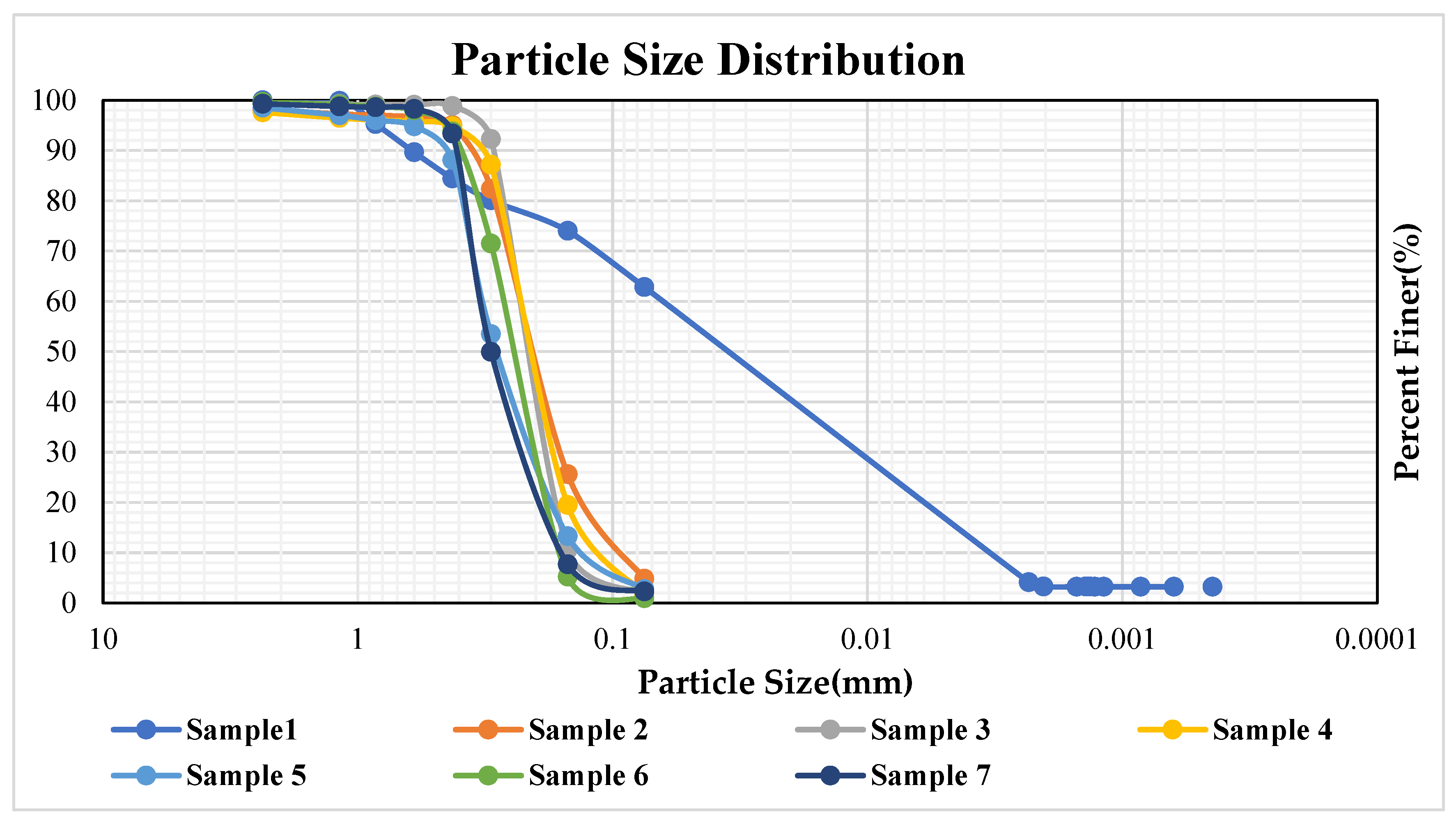
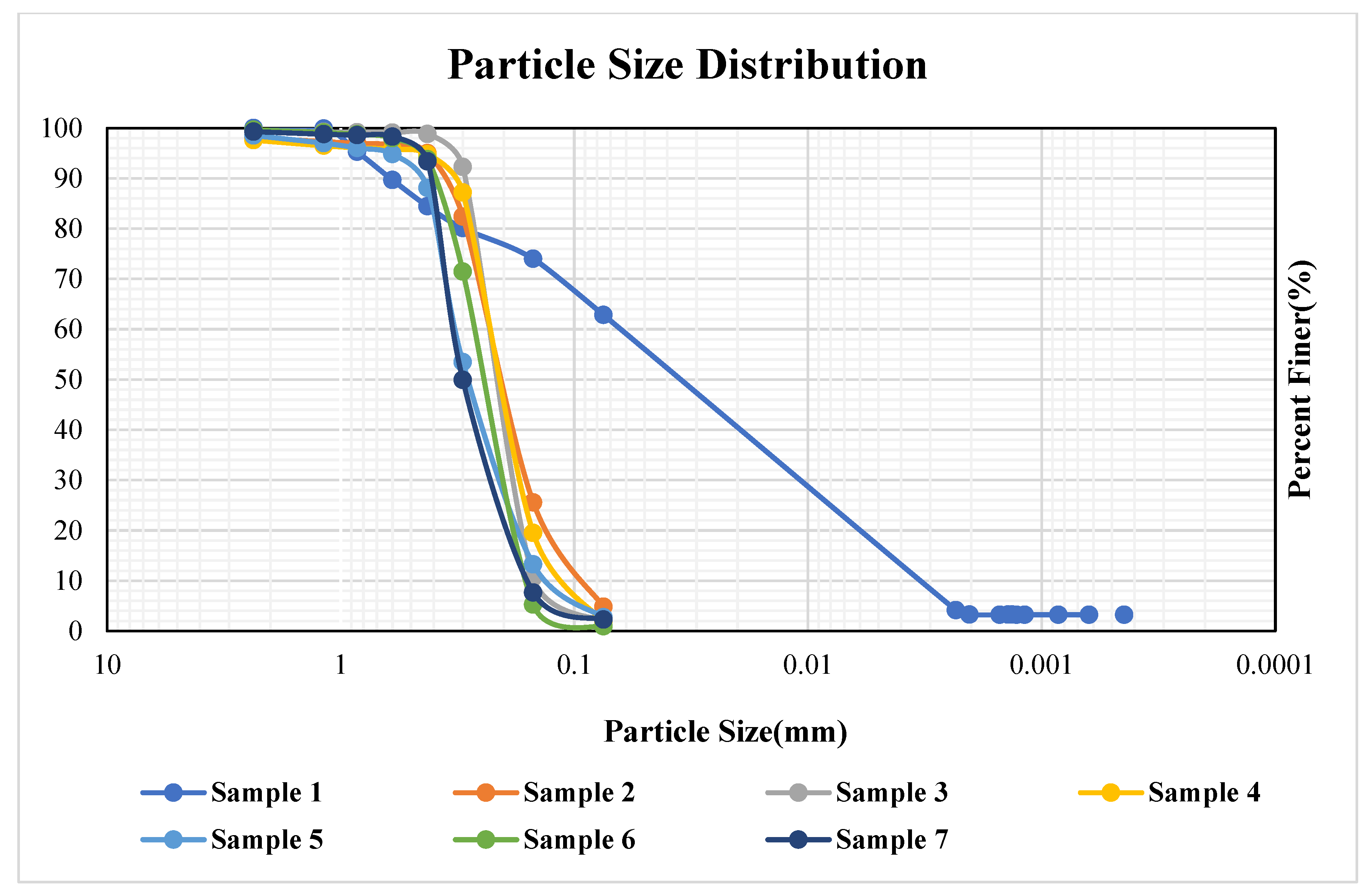
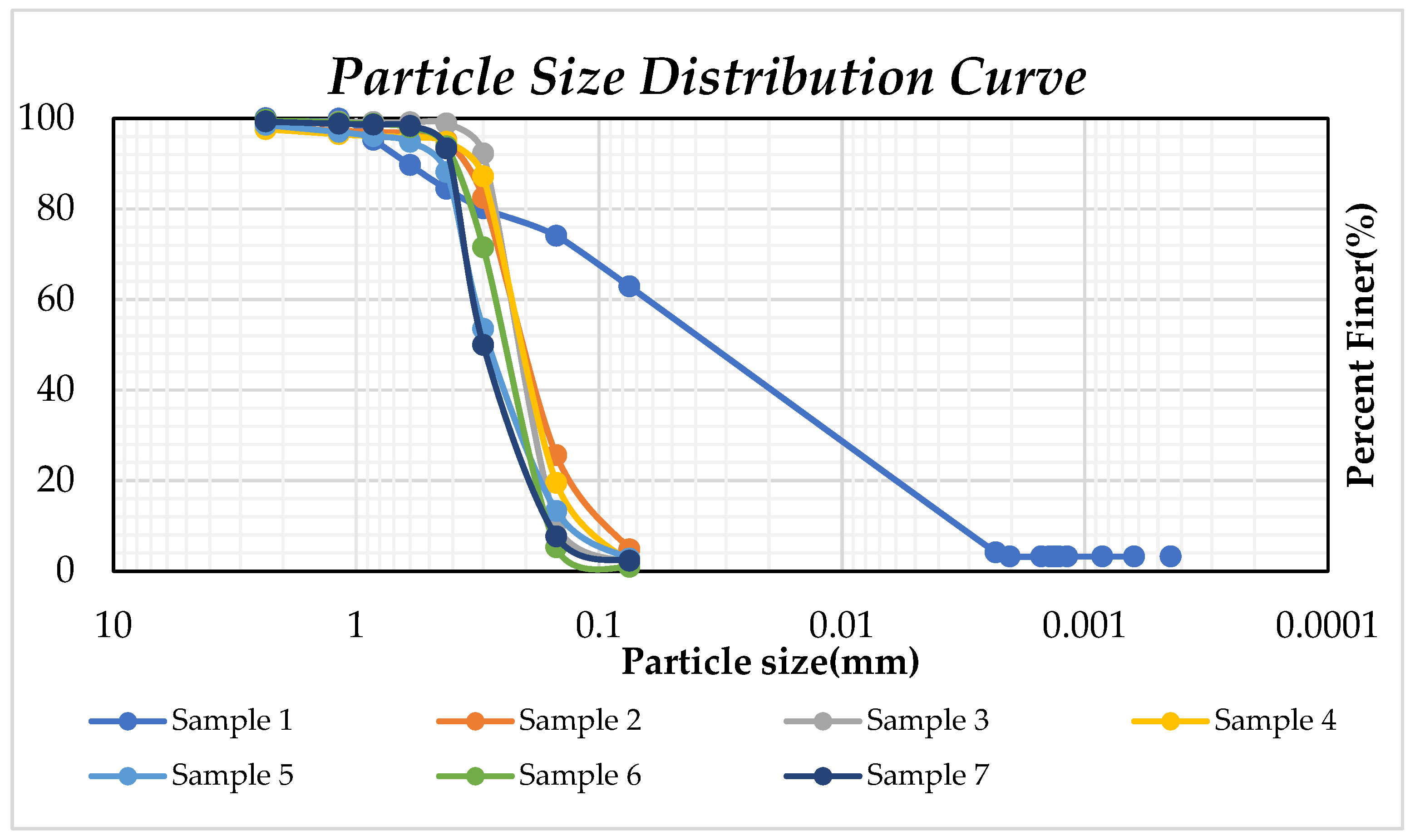
3.1. Sieve Analysis and Hydrometer Analysis

The grain size analysis results provided the soil classification using the mechanical sieve shaker technique and hydrometer analysis. Only one sample is detailed in the

Table 2. Classification of borehole soil samples based on grain size analysis for location 1.

Sample	%Silt	%Clay	%Sand	Classification
1	55	8	37	Silt Loam
2	20	6	74	Sandy Loam
3	8	2.6	89.4	Sand
4	15	5	80	Loamy Sand
5	10	3	87	Sand
6	4.3	1	94.7	Sand
7	6.6	1	92.4	Sand

; the remaining samples of four locations are given in Appendix A. The classification of borehole soil samples based on grain size analysis at location 2, 3, 4, and 5 are showed in Appendix A, respectively, in

Table A1. Classification of borehole soil samples based on grain size analysis at location 2.

Sample	%Silt	%Clay	%Sand	Classification
1	48	10	42	Silt Loam
2	13	2	85	Loamy Sand
3	11	1	89	Sand
4	7	0.5	92.5	Sand
5	20	2	78	Loamy Sand
6	19	2	79	Sand
7	7	0.5	92.5	Sand

,

Table A2. Classification of borehole soil samples based on grain size analysis at location 3.

Sample	%Silt	%Clay	%Sand	Classification
1	61	10	29	Silt Loam
2	5	1	84	Sand
3	6	0.5	93.5	Sand
4	0.5	7	92.5	Sand
5	12	1	87	Sand
6	5	0.2	94.8	Sand
7	4	1	85	Sand

,

Table A3. Classification of borehole soil samples based on grain size analysis at location 4.

Sample	%Silt	%Clay	%Sand	Classification
1	60	10	30	Silt Loam
2	17	3	80	Loamy Sand
3	11	1	89	Sand
4	35	7	58	Sandy Loam
5	10	2	88	Sand
6	8	2	90	Sand
7	5	2	93	Sand

and

Table A4. Classification of borehole soil samples based on grain size analysis at location 5.

Sample	%Silt	%Clay	%Sand	Classification
1	52	9	39	Silt Loam
2	21	5	74	Loamy Sand
3	10	2	88	Sand
4	8	1	91	Sand
5	19	3	88	Loamy Sand
6	22	4	74	Loamy Sand
7	6	1.5	92.5	Sand

. Gradation curves were also drawn to calculate the uniformity coefficient, as shown in Figure 2. The grain size at 10%, 20%, 50%, and 60% was determined, along with the average values of porosity, coefficient of uniformity, and hydraulic conductivity [14]. Figure A1, Figure A2, Figure A3 and Figure A4 in Appendix A show gradation curves, respectively, at locations 2, 3, 4, and 5.

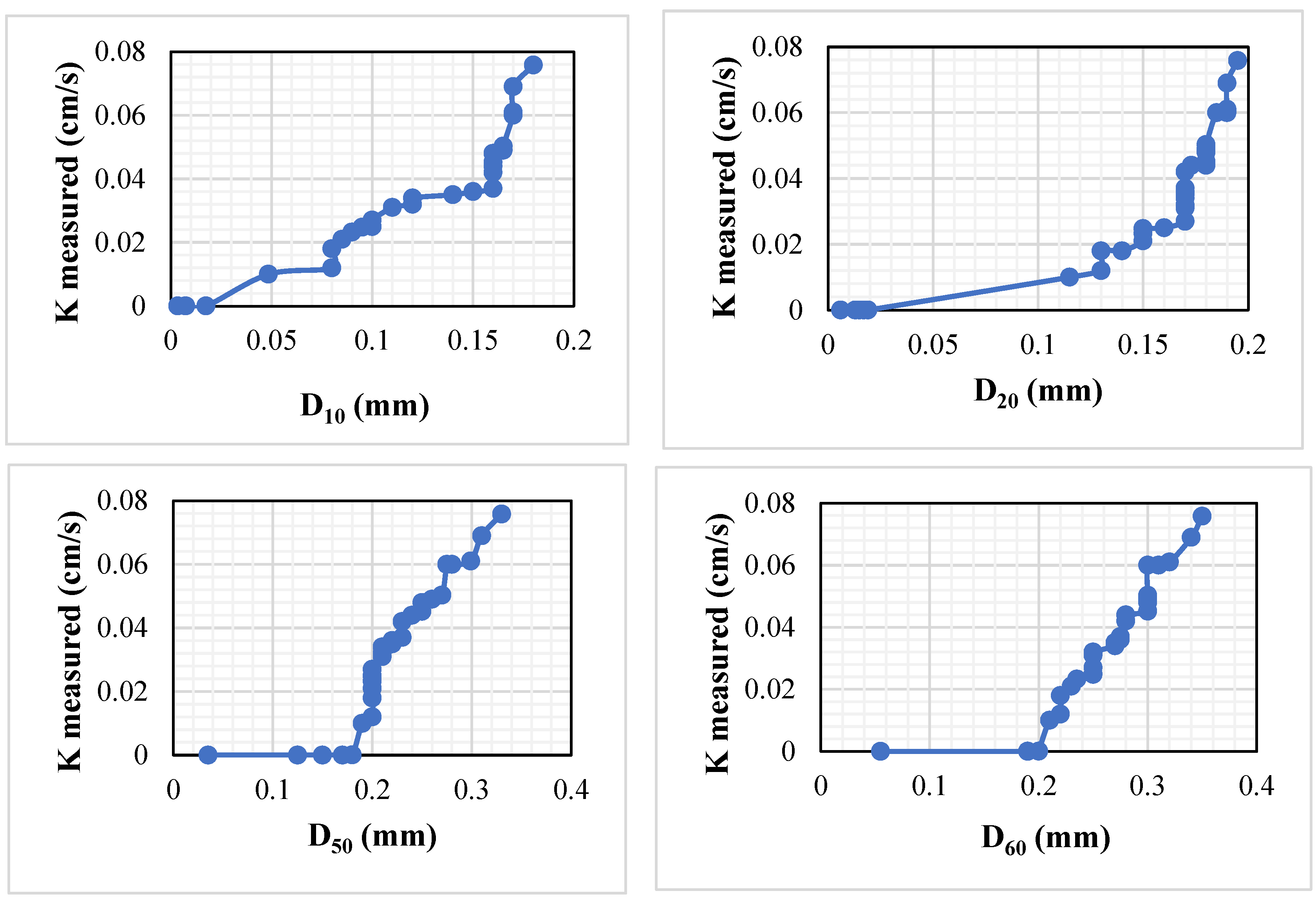
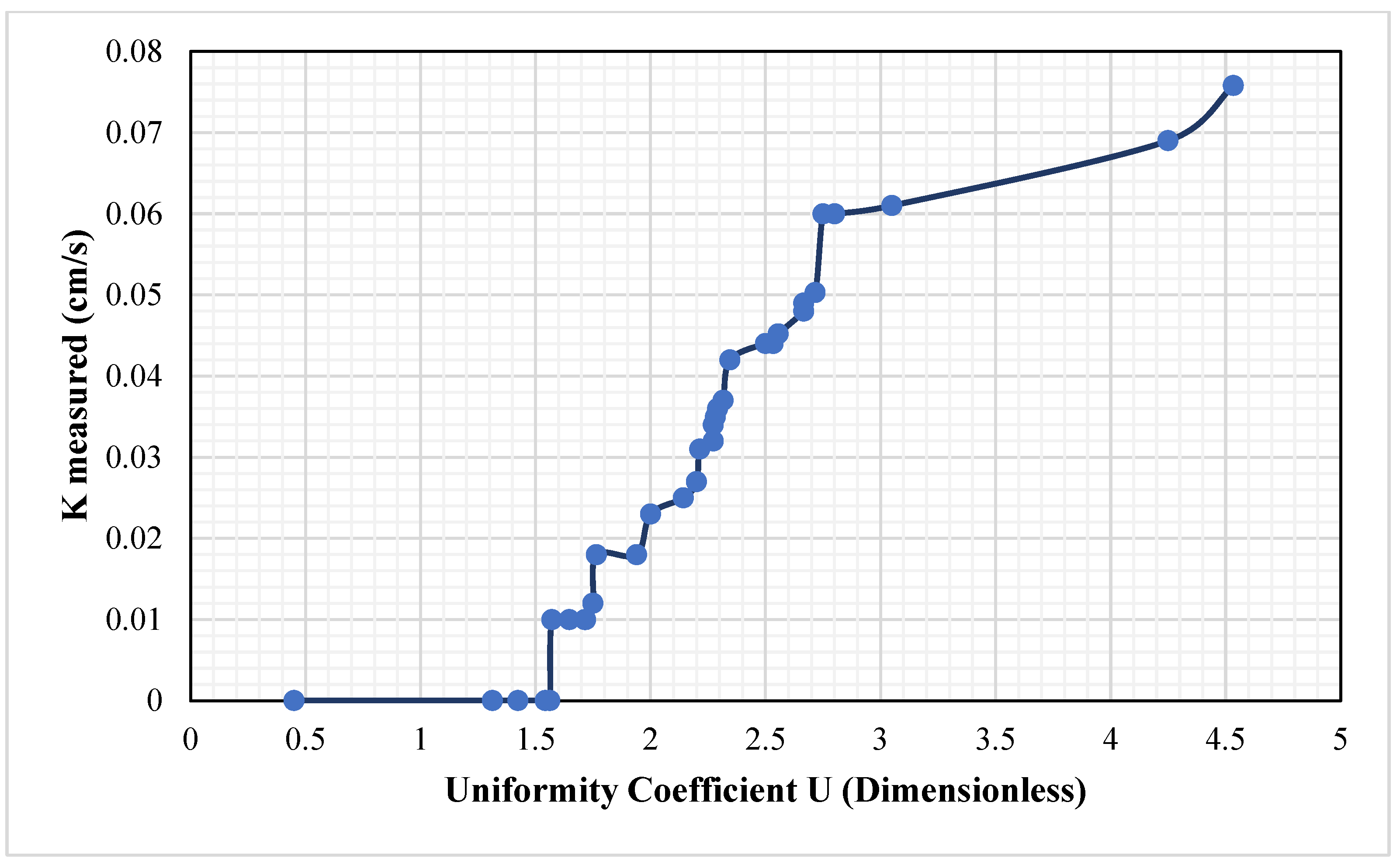
3.2. Relationship of Hydraulic Conductivity with Grain Size, Coefficient of Uniformity, and Porosity

The effect of grain size on hydraulic conductivity was considered in this study. The results showed that, as the effective diameter (D₁₀, D₆₀, D₂₀, D₅₀) increased, the hydraulic conductivity also increased, as mentioned by [1,14]. Initially, when the value of grain size (D₁₀) was small (0.00335 mm), the value of hydraulic conductivity was also small (0.0000307 cm/s). At the middle stage, when the value of D₁₀ increased to 0.095 mm, the value of K increased to 0.023 cm/s. In the end, when the value of D₁₀ increased to 0.17 mm, the value of K decreased to 0.061 cm/s. This decrease in value is due to the presence of clay soil in the sample. Therefore, the other effective grain sizes, such as D₂₀, D₅₀, and D₆₀, followed the same trend shown in Figure 3.

The relationship between the uniformity coefficient and measured hydraulic conductivity was examined, as shown in Figure 4. The relationship revealed that, as the uniformity coefficient increased, the value of hydraulic conductivity also increased. For instance, when the U value was 2.34, K was at 0.042 cm/s. On the other hand, when U was 2.71, the hydraulic conductivity was 0.0503 cm/s. Moreover, the relationship between porosity and K was also determined, as shown in Figure 5. The results indicated that, as the porosity of the borehole soil sample increased, the measured hydraulic conductivity increased. Moreover, the presence of clay soil also affected the porosity as there were fewer pores for clay, so the clayey soil’s porosity value was much lower.

3.3. Estimation of Hydraulic Conductivity Using Empirical Relationship

The grain size analysis of all the samples was very advantageous for determining the applicability of the empirical relationships according to the particular soil. Different significant parameters derived from grain size analysis, such as grain size (D₁₀, D₂₀, D₅₀, and D₆₀), uniformity coefficient (U), and intercept (I), were utilized to compute hydraulic conductivity for all samples by applying nine empirical relationships included in the study. Except for the Terzaghi relationship, which did not apply to the study area, many other studies provided a value of the sorting coefficient β, which was used. The kinematic viscosity obtained using different water temperatures observed between the constant head and falling procedure was used to estimate hydraulic conductivity. Ref. [36]’s formula for both sample 1 and sample 2 was not applicable for all five locations because their values for D₁₀ were less than 0.1 mm, as indicated by [1]. Moreover, the value of the uniformity coefficient for the sample was also greater than 5. Ref. [38] did not apply to any sample because it applied only to the large-grained soils [13]. The [43] formula was not applicable for sample 1 because its d10 value was less than 0.06. The USBR formula could be applied only to medium-grained sand, so it was only applicable for samples 5 and 7. Ref. [46] did not apply to sample 1 because its D₁₀ value was less than 0.06 mm, as shown in

Table 3. Hydraulic conductivity by empirical relationships for location 1.

Hazen (cm/s)	Slitcher (cm/s)	Terzaghi (cm/s)	K-C (cm/s)	Harleman (cm/s)	Beyer (cm/s)	USBR (cm/s)	A&S (cm/s)	Chapius (cm/s)
-	0.00000141	-	0.00000303	0.000014	-	-	0.0000117	-
-	0.0043	-	0.0119	0.0072	0.0155	-	0.0103	0.0071
0.0474	0.0160	-	0.0478	0.0218	0.0508	-	0.0380	0.0212
0.0153	0.0047	-	0.0132	0.0078	0.0168	-	0.0129	0.0795
0.0317	0.0097	-	0.0274	0.0162	0.0349	0.01173	0.0227	0.0134
0.0490	0.0161	-	0.0471	0.0232	0.0527	-	0.0347	0.0210
0.04503	0.0143	-	0.0409	0.0221	0.0490	0.01156	0.0309	0.0185

.

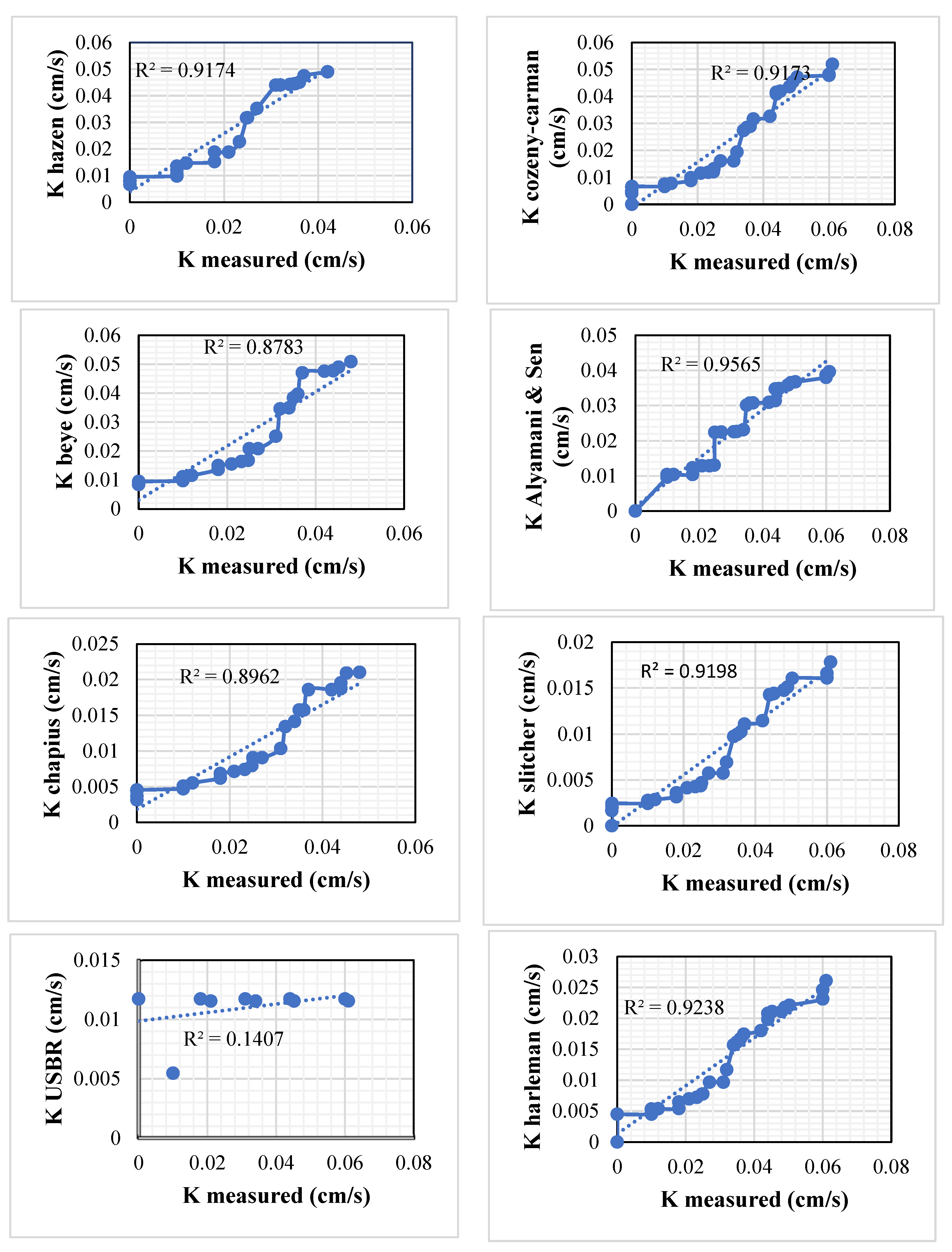
3.4. Comparison of Measured and Empirical Hydraulic Conductivity

When K_measured and K_empirical were considered, it was observed that Kozeny–Carman was the best empirical estimator, but it still overestimated the values. The values determined by the K-C method showed a closer agreement, followed by Allen Hazen and other formulas [1]. Beyer, slitcher, Harleman, and USBR underestimated the values [10].

Table 4. Comparison between experimentally measured and empirical hydraulic conductivity for location 1.

K (lab)	Hazen	Slitcher	K-C	Harleman	Beyer	USBR	A&S	Chapius
0.0000307	-	0.00000141	0.00000303	0.000014	-	-	0.0000117	-
0.02327	-	0.0043	0.0119	0.0072	0.0155	-	0.0103	0.0071
0.0503	0.0474	0.0160	0.0478	0.0218	0.0508	-	0.0380	0.0212
0.0248	0.0153	0.0047	0.0132	0.0078	0.0168	-	0.0129	0.0795
0.0452	0.0317	0.0097	0.0274	0.0162	0.0349	0.01173	0.0227	0.0134
0.0610	0.0490	0.0161	0.0471	0.0232	0.0527	-	0.0347	0.0210
0.0758	0.04503	0.0143	0.0409	0.0221	0.0490	0.01156	0.0309	0.0185

, given below, briefly describes the relationship between lab-measured and empirical K for location, while the rest of the tables are given in Appendix A 

Table A5. Measured hydraulic conductivity (cm/s) of borehole soil samples at different locations.

	Location 2	Location 3	Location 4	Location 5
Sample 1	0.0000107	0.0000113	0.0000185	0.000025
Sample 2	0.044	0.031	0.032	0.069
Sample 3	0.018	0.037	0.034	0.036
Sample 4	0.025	0.018	0.027	0.045
Sample 5	0.055	0.058	0.053	0.06
Sample 6	0.012	0.042	0.021	0.048
Sample 7	0.035	0.049	0.044	0.06

.

Figure 6 shows a difference between the observed and computed hydraulic conductivity. As mentioned above, Kozeny–Carman was the best calculator for hydraulic conductivity among the empirical ones, but it still overestimated the value of hydraulic conductivity. For instance, the measured value of K for sample 1 is 3.07 × 10⁻⁵, while K-C is 3.03 × 10⁻⁶. This is around 0.02 for K measured and 0.011 for K-C for sample 2. All remaining samples exhibit the same variation. The Hazen formula and Alyamani and Sen formulae were the best estimators after the K-C relationship and indicated the approximate values, as shown in

Table 5. Correlation analysis of dimensionless parameters of the sandy sample.

	K Measured	U	Porosity (n)	D50
K measured	1
U	0.015033	1
Porosity (n)	0.045516	−0.9386189	1
D50	−0.19974	0.31038783	−0.19459	1

. However, the Hazen formula was inapplicable for samples 1 and 2, but was applicable for other samples. Meanwhile, K measured for sample 3 equals 0.05, and K (Hazen) equals 0.047 cm/s. Moreover, for sample 4, K measured is 0.02 and K (Hazen) is 0.015 cm/s. All the remaining formulas either overestimate or underestimate the hydraulic conductivity values for different soil samples [1,12,29].

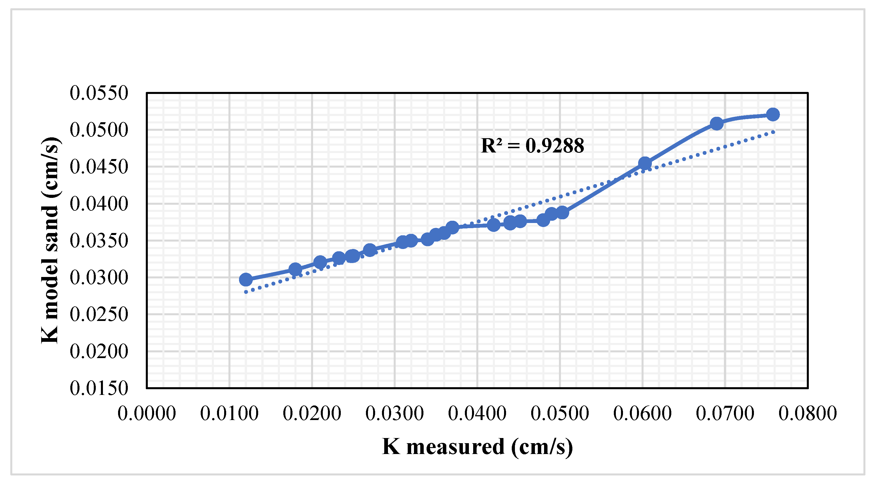
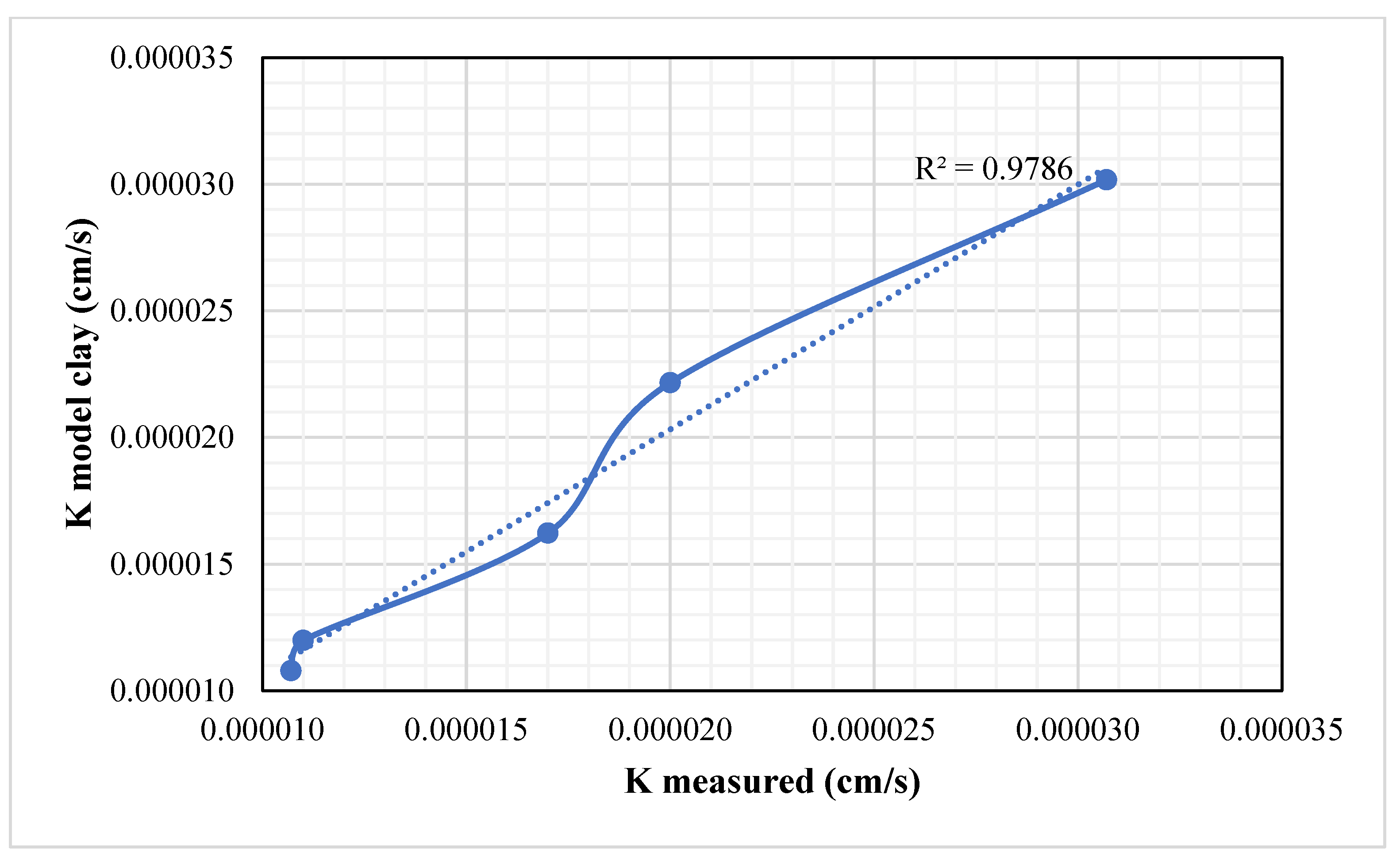
3.5. Development of Statistical Model

A correlation analysis was performed to determine which soil characteristics affect the dependent variable of hydraulic conductivity. The Table 5 and

Table 6. Correlation analysis of dimensionless parameters of the clayey sample.

	U	Porosity (n)	D50	K Measured
U	1
Porosity (n)	0.763178093	1
D50	0.862107974	0.448747	1
K measured	0.805867619	0.974282	0.5111618	th1

display the findings of the correlation study for sandy and clayey soil samples. The soil’s porosity, U, and D₅₀ significantly influenced the hydraulic conductivity, as indicated by [15].

The statistical model for the hydraulic conductivity of sandy and clayey soil was then developed using a regression analysis between grain size, porosity, and the uniformity coefficient. The total number of samples was 35, of which 30 were sandy soils and 5 were clayey. Hence, the data from 30 sandy samples were analyzed using the statistical model for sandy soil, while the clayey model analyzed the data from 5 clayey samples. The data analysis was carried out with MS Excel 16’s toolbox. Below are the models for both clay and sand:

$$K\left(Sand\right)=U\ast \left(0.01895\right)+D_{50}\ast (-0.09992)+n\ast \left(0.663921\right)+(-0.233518)$$

(12)

$$K\left(Clay\right)=U\ast \left(0.000005164\right)+D_{50}\ast \left(-0.000008653\right)+n\ast \left(0.000904572\right)+(-0.0003256)$$

(13)

where K(Sand) is the hydraulic conductivity of sand (cm/s), K(Clay) is the hydraulic conductivity of clay (cm/s), U is the coefficient of uniformity (dimensionless), n is the porosity (dimensionless), and D₅₀ is the effective grain sizes (mm) 50% finer.

Figure 7 compares the measured hydraulic conductivity values with those developed using the sandy soil model. The plot reveals that the data points are concentrated closer to the agreement line, indicating a higher degree of agreement between the two sets of values. The comparison of the measured hydraulic conductivity of clayey samples and hydraulic conductivity measured by the clayey model is given below in Figure 8. Furthermore, the statistical model for both sand and clayey soil is found to have generated more accurate values compared to those computed using an empirical relationship.

To assess the accuracy of the results, statistical evaluation tests were conducted on the lab-measured hydraulic conductivity values, the empirically measured values, and the model-measured hydraulic conductivity values. These tests are summarized in

Table 7. Evaluation of statistical parameters for hydraulic conductivity.

Statistical Parameter	RMSE (cm/s)	MAE (cm/s)	Cc (Dimensionless)
Hazen	0.007	0.006	0.917
Kozeny–Carman	0.008	0.007	0.917
Slitcher	0.025	0.021	0.45
Alyamani and Sen	0.01	0.007	0.956
Harleman et al.	0.019	0.017	0.924
Beyer	0.006	0.05	0.889
USBR	0.01	0.009	0.423
Chapius et al.	0.017	0.014	0.906
Developed model	0.013	0.0011	0.927

.

Appendix A Table A5 shows the measured hydraulic conductivity of borehole soil samples at different locations.

4. Conclusions

This study assessed the measured hydraulic conductivity of porous media alongside nine empirical formulas. This study also examined how soil properties like porosity, uniformity coefficient, and grain size affect hydraulic conductivity. Given the exceptionally low porosity and particle size values of clayey soil, it was determined that the hydraulic conductivity for the soil was exceedingly low for both empirical equations and the measured hydraulic conductivity. According to experimental results, borehole soil sample hydraulic conductivity increases with grain size, uniformity coefficient, and porosity. Although the Kozeny–Carman connection overestimated the value of hydraulic conductivity, it was determined to have the most accurate agreement between the empirical relationship and the observed hydraulic conductivity. The Slichter, Terzaghi, Harleman, et al., USBR, and Chapuis relationships underestimated the hydraulic conductivity of borehole soil samples.

In contrast, the Kozeny–Carman relationship and the Beyer, Hazen, and Alyamani and Sen relationships predict hydraulic conductivity values in close agreement with experimentally determined values. Compared to the hydraulic conductivity determined by empirical relationships, the hydraulic conductivity predicted by the sandy and clayey models demonstrated significant agreement with the measured values. The model’s hydraulic conductivity was found to have acceptable values for the statistical parameters RMSE, MAE, and Cc, which were 0.013, 0.927, and 0.0011, respectively.

References

1. Chandel, A.; Shankar, V. Evaluation of empirical relationships to estimate the hydraulic conductivity of borehole soil samples. Hydraul. Eng. 2021, 28, 368–377. [Google Scholar] [CrossRef]
2. Albano, R.; Lacava, T.; Mazzariello, A.; Manfreda, S.; Adamowski, J.; Sole, A. How Can Seasonality Influence the Performance of Recent Microwave Satellite Soil Moisture Products? Remote Sens. 2024, 16, 3044. [Google Scholar] [CrossRef]
3. Albano, R.; Manfreda, S.; Celano, G. MY SIRR: Minimalist agro-hYdrological model for Sustainable IRRigation management—Soil moisture and crop dynamics. SoftwareX 2017, 6, 107–117. [Google Scholar] [CrossRef]
4. Mazzariello, A.; Albano, R.; Lacava, T.; Manfreda, S.; Sole, A. Intercomparison of recent microwave satellite soil moisture products on European ecoregions. J. Hydrol. 2023, 626, 130311. [Google Scholar] [CrossRef]
5. Říha, J.; Petrula, L.; Hala, M.; Alhasan, Z. Assessment of empirical formulae for determining the hydraulic conductivity of glass beads. J. Hydrol. Hydromech. 2018, 66, 337–347. [Google Scholar] [CrossRef]
6. Rosas, J.; Lopez, O.; Missimer, T.M.; Coulibaly, K.M.; Dehwah, A.H.; Sesler, K.; Lujan, L.R.; Mantilla, D. Determination of hydraulic conductivity from grain-size distribution for different depositional environments. Groundwater 2014, 52, 399–413. [Google Scholar] [CrossRef]
7. Goodarzi, M.R.; Vazirian, M.; Niazkar, M. Hydraulic Conductivity Estimation: Comparison of Empirical Formulas Based on New Laboratory Experiments. Water 2024, 16, 1854. [Google Scholar] [CrossRef]
8. Hong, B.; Li, X.; Wang, L.; Li, L.; Xue, Q.; Meng, J. Using the effective void ratio and specific surface area in the Kozeny–Carman equation to predict the hydraulic conductivity of loess. Water 2019, 12, 24. [Google Scholar] [CrossRef]
9. Chandel, A.; Shankar, V.; Alam, M.A. Experimental investigations for assessing the influence of fly ash on the flowthrough porousmedia in Darcy regime. Water Sci. Technol. 2021, 83, 1028–1038. [Google Scholar] [CrossRef]
10. Cheng, C.; Chen, X. Evaluation of methods for determination of hydraulic properties in an aquifer–aquitard system hydrologically connected to a river. Hydrogeol. J. 2007, 15, 669–678. [Google Scholar] [CrossRef]
11. Odong, J. Evaluation of empirical formulae for determination of hydraulic conductivity based on grain-size analysis. J. Am. Sci. 2007, 3, 54–60. [Google Scholar]
12. Song, J.; Chen, X.; Cheng, C.; Wang, D.; Lackey, S.; Xu, Z. Feasibility of grain-size analysis methods for determination of vertical hydraulic conductivity of streambeds. J. Hydrol. 2009, 375, 428–437. [Google Scholar] [CrossRef]
13. Ishaku, J.M.; Gadzama, E.W.; Kaigama, U. Evaluation of empirical formulae for the determination of hydraulic conductivity based on grain-size analysis. J. Geol. Min. Res. 2011, 3, 105–113. [Google Scholar]
14. Pliakas, F.; Petalas, C. Determination of Hydraulic Conductivity of Unconsolidated River Alluvium from Permeameter Tests, Empirical Formulas and Statistical Parameters Effect Analysis. Water Resour. Manag. 2011, 25, 2877–2899. [Google Scholar] [CrossRef]
15. Yoon, S.; Lee, S.R.; Kim, Y.T.; Go, G.H. Estimation of saturated hydraulic conductivity of Korean weathered granite soils using a regression analysis. Geomech. Eng. 2015, 9, 101–113. [Google Scholar] [CrossRef]
16. Naeej, M.; Naeej, M.R.; Salehi, J.; Rahimi, R. Hydraulic conductivity prediction based on grain-size distribution using M5 model tree. Geomech. Geoengin. 2017, 12, 107–114. [Google Scholar] [CrossRef]
17. Obianyo, J.I. Investigation of Empirical Models for Hydraulic Conductivity from Grain-size Distribution 1 1 Obianyo J.I. and 1 Eboh. FUPRE J. Sci. Ind. Res. 2020, 4, 60–70. [Google Scholar]
18. Muhammad, S.; Ehsan, M.I.; Khalid, P. Optimizing exploration of quality groundwater through geophysical investigations in district Pakpattan, Punjab, Pakistan. Arab. J. Geosci. 2022, 15, 721. [Google Scholar] [CrossRef]
19. Bhutta, M.N.; Smedema, L.K. One hundred years of waterlogging and salinity control in the Indus valley, Pakistan: A historical review. Irrig. Drain. J. Int. Comm. Irrig. Drain. 2007, 56, S81–S90. [Google Scholar] [CrossRef]
20. Sikandar, P.; Bakhsh, A.; Arshad, M.; Rana, T. The use of vertical electrical sounding resistivity method for the location of low salinity groundwater for irrigation in Chaj and Rachna Doabs. Environ. Earth Sci. 2010, 60, 1113–1129. [Google Scholar] [CrossRef]
21. Hasan, M.; Shang, Y.; Akhter, G.; Jin, W. Delineation of contaminated aquifers using integrated geophysical methods in Northeast Punjab, Pakistan. Environ. Monit. Assess. 2020, 192, 12. [Google Scholar] [CrossRef] [PubMed]
22. Zakir-Hassan, G.; Hassan, F.R.; Punthakey, J.; Shabir, G. Challenges for groundwater-irrigated agriculture and management opportunities in Punjab province of Pakistan. Int. J. Agric. Nutr. 2022, 4, 61–73. [Google Scholar] [CrossRef]
23. Qureshi, A.S. Challenges and opportunities of groundwater management in Pakistan. In Groundwater of South Asia; Springer: Berlin/Heidelberg, Germany, 2018; pp. 735–757. [Google Scholar]
24. Watto, M.A.; Mugera, A.W. Groundwater depletion in the Indus Plains of Pakistan: Imperatives, repercussions and management issues. Int. J. River Basin Manag. 2016, 14, 447–458. [Google Scholar] [CrossRef]
25. Razzaq, A.; Liu, H.; Xiao, M.; Mehmood, K.; Shahzad, M.A.; Zhou, Y. Analyzing past and future trends in Pakistan’s groundwater irrigation development: Implications for environmental sustainability and food security. Environ. Sci. Pollut. Res. 2023, 30, 35413–35429. [Google Scholar] [CrossRef]
26. Ashiq, M.M.; Rehman, H.U.; Khan, N.M. Impact of large diameter recharge wells for reducing groundwater depletion rates in an urban area of Lahore, Pakistan. Environ. Earth Sci. 2020, 79, 403. [Google Scholar] [CrossRef]
27. Qureshi, A.S. Improving food security and livelihood resilience through groundwater management in Pakistan. Glob. Adv. Res. J. Agric. Sci. 2015, 4, 687–710. [Google Scholar]
28. Iqbal, J.; Su, C.; Rashid, A.; Yang, N.; Baloch, M.Y.; Talpur, S.A.; Ullah, Z.; Rahman, G.; Rahman, N.U.; Sajjad, M.M. Hydrogeochemical assessment of groundwater and suitability analysis for domestic and agricultural utility in southern Punjab, Pakistan. Water 2021, 13, 3589. [Google Scholar] [CrossRef]
29. Lytton, B.S.L.; Ali, A.; Garthwaite, B.; Punthakey, J.F. Groundwater in Pakistan’s Indus Basin: Present and Future Prospects. 2021. Available online: https://documents.worldbank.org/en/publication/documents-reports/documentdetail/501941611237298661/groundwater-in-pakistan-s-indus-basin-present-and-future-prospects (accessed on 20 December 2024).
30. Qureshi, A.S. Groundwater governance in pakistan: From colossal development to neglected management. Water 2020, 12, 3017. [Google Scholar] [CrossRef]
31. Carter, M.R.; Gregorich, E.G. Soil Sampling and Methods of Analysis; CRC Press: Boca Raton, FL, USA, 2007. [Google Scholar]
32. KR, A.D. Soil Mechanics and Foundation Engineering, 6th ed.; Standard Publishers Distributors: Delhi, India, 2006; pp. 14–22. [Google Scholar]
33. ASTM D7928; Soil Hydrometer Testing: Sedimentation Method Techniques & Equipment. ASTM: West Conshohocken, PA, USA, 2007.
34. ASTM D2434-19; Standard Test Method for Permeability of Granular Soils (Constant Head). ASTM: West Conshohocken, PA, USA, 2009.
35. Rushton, K.R. Groundwater Hydrology: Conceptual and Computational Models; John Wiley & Sons: Hoboken, NJ, USA, 2004. [Google Scholar] [CrossRef]
36. Hazen, A. Some physical properties of sand gravel with special reference to their use in filtration. In State Sanitation: A Review of the Work of the Massachusetts State Board of Health Volume II; Harvard University Press: Cambridge, MA, USA; London, UK, 1917; pp. 232–248. [Google Scholar]
37. Slichter, C.S. Theoretical Investigation of the Motion of Ground Waters; U.S. Department of the Interior, Geological Survey, Water Resources Division, Ground Water Branch: Olivette, MO, USA, 1899; pp. 295–384. [Google Scholar]
38. Terzaghi, K. Principles of soil mechanics III—Determination of Permeability of Clay. Eng. News-Rec. 1925, 95, 19–27. [Google Scholar]
39. Carman, P.C. Flow of Gases Through Porous Media; Academic Press Inc.: New York, NY, USA, 1956. [Google Scholar]
40. Carman, P.C. Fluid flow through granular beds. Trans. Inst. Chem. Eng. 1937, 15, 150–166. [Google Scholar] [CrossRef]
41. Kozeny, J. Via capillary conduit the water in the ground. R. Acad. Sci. Vienna Proc. Cl. I 1927, 136, 271–306. [Google Scholar]
42. Harleman, D.R.F.; Mehlhorn, P.F.; Rumer, R.R., Jr. Dispersion-permeability correlation in porous media. J. Hydraul. Div. 1963, 89, 67–85. [Google Scholar] [CrossRef]
43. Beyer, W. On the determination of hydraulic conductivity of gravels and sands from grain-size distributions. Wasserwirtsch.-Wassertech. 1964, 14, 165–169. [Google Scholar]
44. Cudworth, A.G. Flood Hydrology Manual: A Water Resources Technical Publication; U.S. Department of the Interior, Bureau of Reclamation: Denver, CO, USA, 1989. [Google Scholar]
45. Alyamani, M.S.; Şen, Z. Determination of hydraulic conductivity from complete grain-size distribution curves. Groundwater 1993, 31, 551–555. [Google Scholar] [CrossRef]
46. Chapuis, R.P.; Dallaire, V.; Marcotte, D.; Chouteau, M.; Acevedo, N.; Gagnon, F. Evaluating the hydraulic conductivity at three different scales within an unconfined sand aquifer at Lachenaie, Quebec. Can. Geotech. J. 2005, 42, 1212–1220. [Google Scholar] [CrossRef]
47. Sepahvand, A.; Singh, B.; Sihag, P.; Samani, A.N.; Ahmadi, H.; Nia, S.F. Assessment of the various soft computing techniques to predict sodium absorption ratio (SAR). ISH J. Hydraul. Eng. 2021, 27, 124–135. [Google Scholar] [CrossRef]
48. Sihag, P.; Singh, V.P.; Angelaki, A.; Kumar, V.; Sepahvand, A.; Golia, E. Modelling of infiltration using artificial intelligence techniques in semi-arid Iran. Hydrol. Sci. J. 2019, 64, 1647–1658. [Google Scholar] [CrossRef]
Figure 1. Study area boring location map.
Hydrology 12 00055 g001
Figure 2. Particle size distribution of borehole soil samples at bore 1.
Hydrology 12 00055 g002
Figure 3. Variation between grain size and hydraulic conductivity.
Hydrology 12 00055 g003
Figure 4. Relationship between uniformity coefficient and K (measured).
Hydrology 12 00055 g004
Figure 5. Variation between porosity and hydraulic conductivity.
Hydrology 12 00055 g005
Figure 6. Comparison between experimentally measured and calculated hydraulic conductivity.
Hydrology 12 00055 g006
Figure 7. Comparison between K (measured) and K (sand model).
Hydrology 12 00055 g007
Figure 8. Comparison between K (measured) and K (clayey model).
Hydrology 12 00055 g008