
A Null Space Sensitivity Analysis for Hydrological Data Assimilation with Ensemble Methods


Abstract
:1. Introduction
2. Data and Methods
2.1. Study Site, Observations, and Models
- Changing weather patterns, particularly increased drought frequency and magnitude, resulting from global climate change;
- Increased water demands in this rapidly growing and developing portion of the San Antonio–Austin corridor.
- Water elevations observed in wells are available upon request from the agencies listed in Table A3. Expectations for uncertainty and observation error are generated as follows.
- –
- At the time of data processing for this study in 2021, there were no dedicated monitoring well or piezometer observations available in the study area. All water level observations came from wells that are, or may be, pumped with some unknown frequency.
- –
- Most of the agencies listed in Table A3 do not have the resources and funding to collect location surveys, which are stamped by a registered surveyor, and generate scientific data products that include cleaned, filtered, and verified recodes based on published data standards in addition to raw field observations.
- –
- Many water level observations are available as point-in-time observations that occur sporadically with a month or more separating measurements.
- –
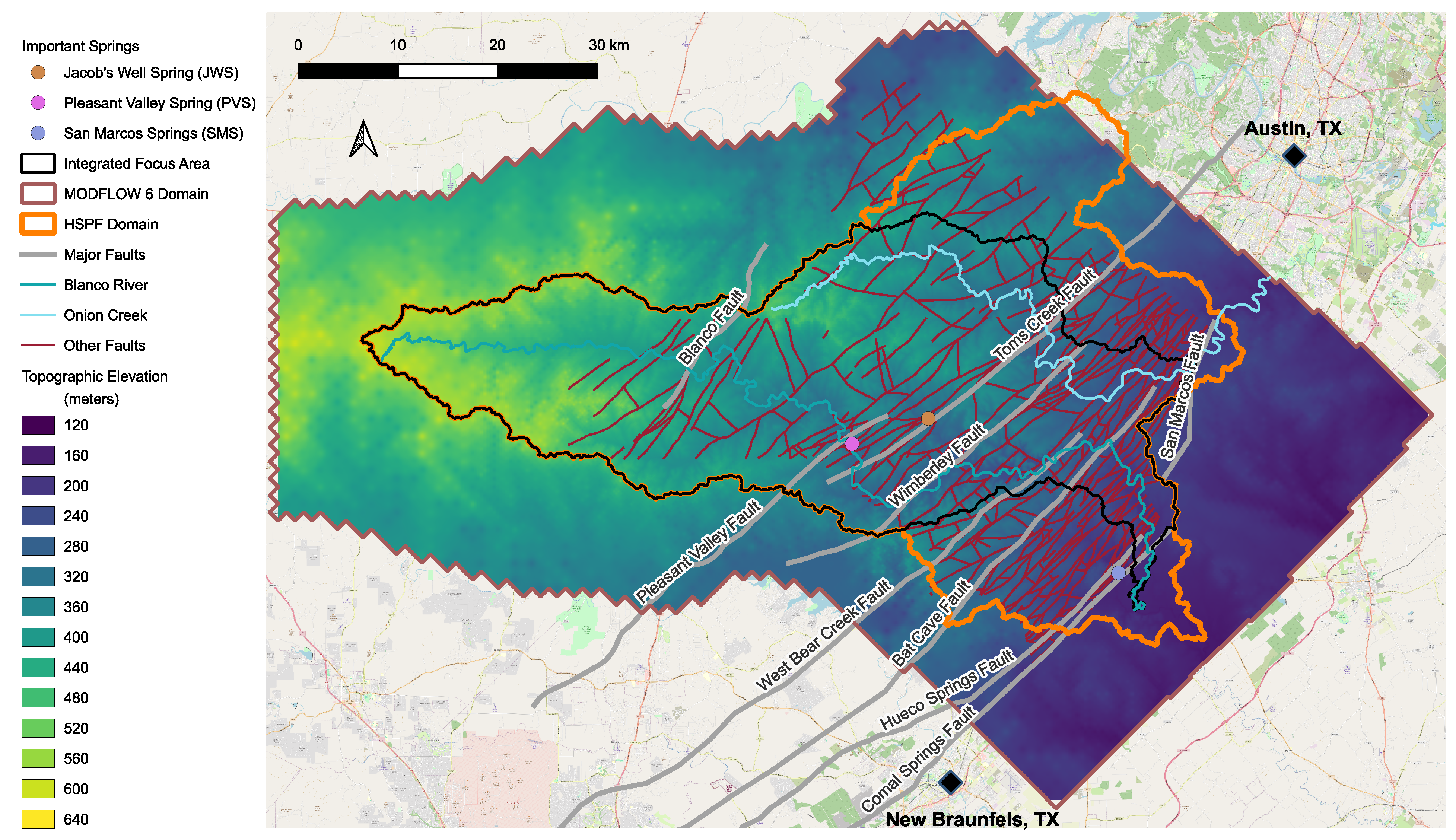
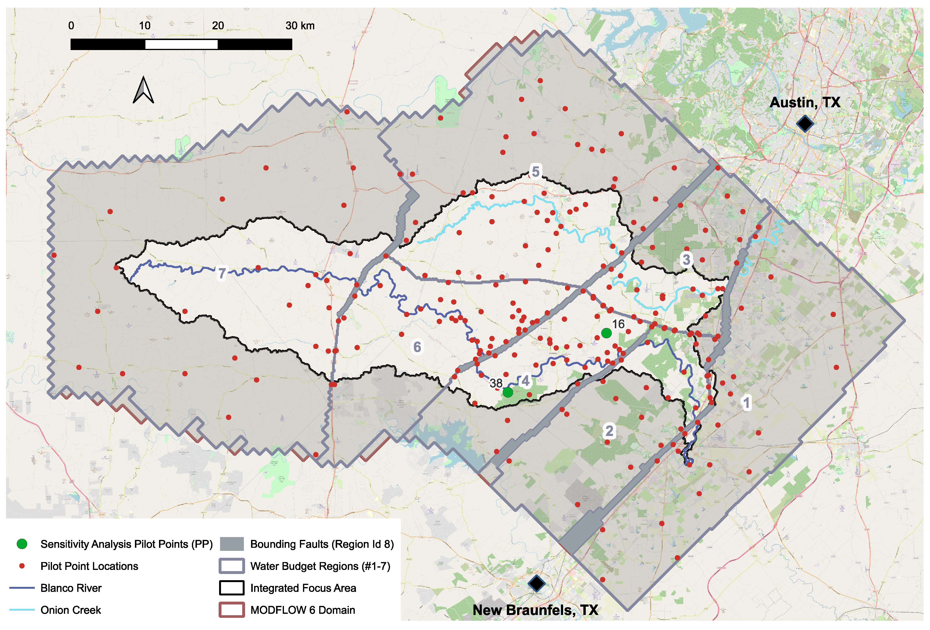
- Figure 2 shows the locations of 96 wells with water level observations within the study area and identifies sparse spatial coverage for these well-based observations. The Middle Trinity Aquifer has by far the largest number of wells in the focus area, with 53. The focus area is the “Integrated Focus Area” in Figure 2. The other three aquifers examined (the Balcones Fault Zone (BFZ) Edwards Aquifer, Upper Trinity Aquifer, and Lower Trinity Aquifer) have three wells each within the focus area. For the Middle Trinity Aquifer, 53 wells in the focus area correspond to an average density of one observation location per 40.5 km2.
- Stream discharge estimates are available from the data portals identified in Table A2. Ref. [19] provides a detailed uncertainty analysis for the BRAAT project and the 16 gauging stations shown in Figure 2. The limitations of these data sets are summarized below.
- –
- Water stage recorders, which measure the static water level in the stream or river, and a rating curve are used to calculate discharge at each of these stations. Expected measurement errors for discharge calculated using a rating curve are ±50–100% for low flows, ±10–20% for medium or high in-bank flows, and ±40% for out-of-bank flows [20]. A rating curve provides an empirical and poor-quality hydrodynamics model [19].
- –
- Only 2 out of 16 stations have Water Year (WY) 2021 data quality assessed as “good”. The other 14 stations have “fair” to “poor” data quality assessments [19].
- –
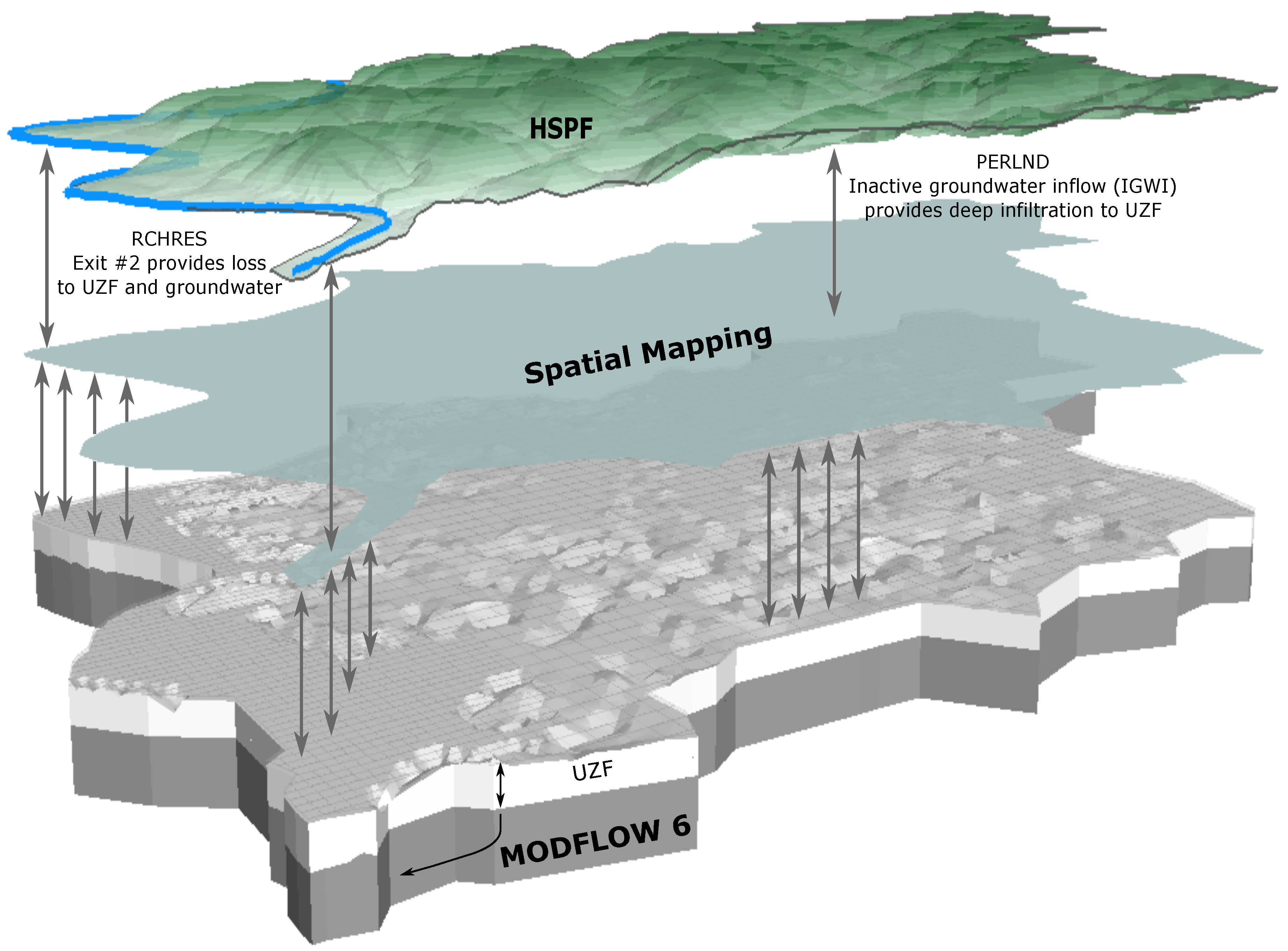
- The Hydrological Simulation Program–FORTRAN (HSPF) represents water movement and storage in watersheds, rivers, and creeks.
- –
- The “Blanco River Water Budget Basin” and “Onion Creek Water Budget Basin” in Figure 3 are the budget accounting areas for surface water and the HSPF model.
- MODFLOW 6 simulates groundwater movement and storage.
- –
- The Unsaturated Zone Flow (UZF) advanced stress package from MODFLOW 6 links HSPF and MODFLOW 6 and represents variably saturated zone considerations.
- –
- Because UZF links groundwater with surface water, it contributes to water budget accounting in both water budget basins and water budget regions.
2.2. Hydrological and Hydrodynamical Model Representations
2.3. Data Assimilation (DA)
- Inherent prior parameter uncertainty, , from limitations in scientific understanding;
- Data insufficiency caused by insufficient information within the observed data set of important outcomes, i.e., target observations, to significantly reduce parameter uncertainty. In other words, available data may be insufficient to condition the range parameter values from the naturally diffuse prior range;
- Observation errors consisting of observation measurement errors and model representation errors. They can be explicitly represented in DA using an observation error model.
2.3.1. Ensemble Methods
- Ensemble methods can cope with higher levels of non-linearity in the parameter–output relationship compared to derivative methods.
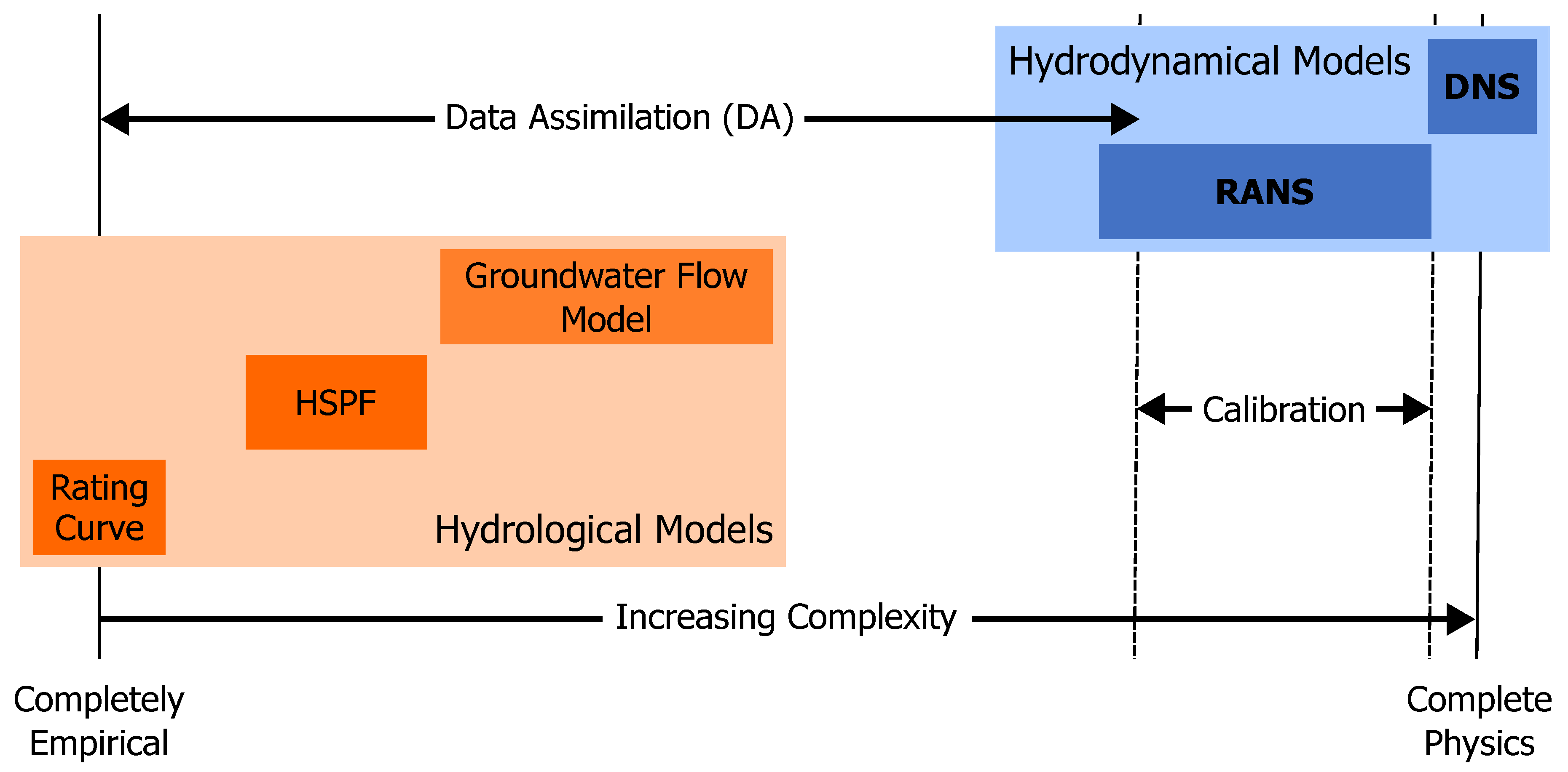
- Watershed and surface water numerical models tend to have significant non-linearities because of the hyperbolic nature of the governing physical equations, i.e., DNS and RANS.
- The empirical relationships between volume and discharge in HSPF for the BRAAT project were designed to be non-linear to address competing demands between river discharge downstream and seepage loss discharge.
- They tend to be relatively efficient computationally when dealing with very large numbers of parameters, which are commonly encountered in applied groundwater modeling.
- MODFLOW 6 represents groundwater flow using a PDE form of continuity. PDE models require that parameters be specified for every cell or node in the computational grid and are highly parameterized models because they have large numbers of parameters.
- For the BRAAT project, the MODFLOW 6 model has 2,324,780 active cells. Five parameters (hydraulic conductivity in the x-direction, , hydraulic conductivity in the y-direction, , hydraulic conductivity in the z-direction, , specific storage, , and specific yield, ) are specified for each active cell, which results in the possibility of 11,623,900 flow property parameters in the absence of regularization.
- PESTPP-IES provides explicit incorporation of many forms of observation error models, which account for observation error and model representation error, into the assimilation process.
- Observation error models for this effort are discussed in Section 2.3.2.
- A significant observation error is expected for the observations available in the study area, as discussed in Section 2.1.
- Hydrological models are used in the integrated hydrological modeling, as discussed in Section 2.2. Hydrological models entail expectations of approximate solutions without high-resolution accuracy and precision, which means that significant model representation error is expected.
- Some 184 UZF parameter values were optimized during assimilation, as shown in Table A5.
- Some 409 HSPF parameter values, all of which relate to empirical relationships between volume and discharge in hydrological routing, were optimized, as listed in Table A5. These 409 parameters represent individual rows in 48 volume-to-discharge lookup tables, or FTABLES. Consequently, there are only 48 empirical lookup tables that internally have a few rows that vary during assimilation.
- A total of 4746 MODFLOW 6 parameters were constrained as part of DA, as listed in Table A6.
2.3.2. Observation Error Models
2.3.3. Complexity and the Bias–Variance Tradeoff
- Regularization to reduce HSPF model complexity
- –
- A standalone HSPF-only assimilation was conducted prior to the integrated model training. The watershed parameters listed in Table A7 were optimized during this preliminary assimilation and then fixed for integrated hydrological model assimilation. The result is that only 409 HSPF parameter values were varied during integrated hydrological model assimilation.
- Four regularization techniques provided reduction in number of assimilated parameters from more than eleven million to less than five thousand for the MODFLOW 6 model component. Additional details are provided in Appendix A.2.3.
- Regionalization into seven water budget regions;
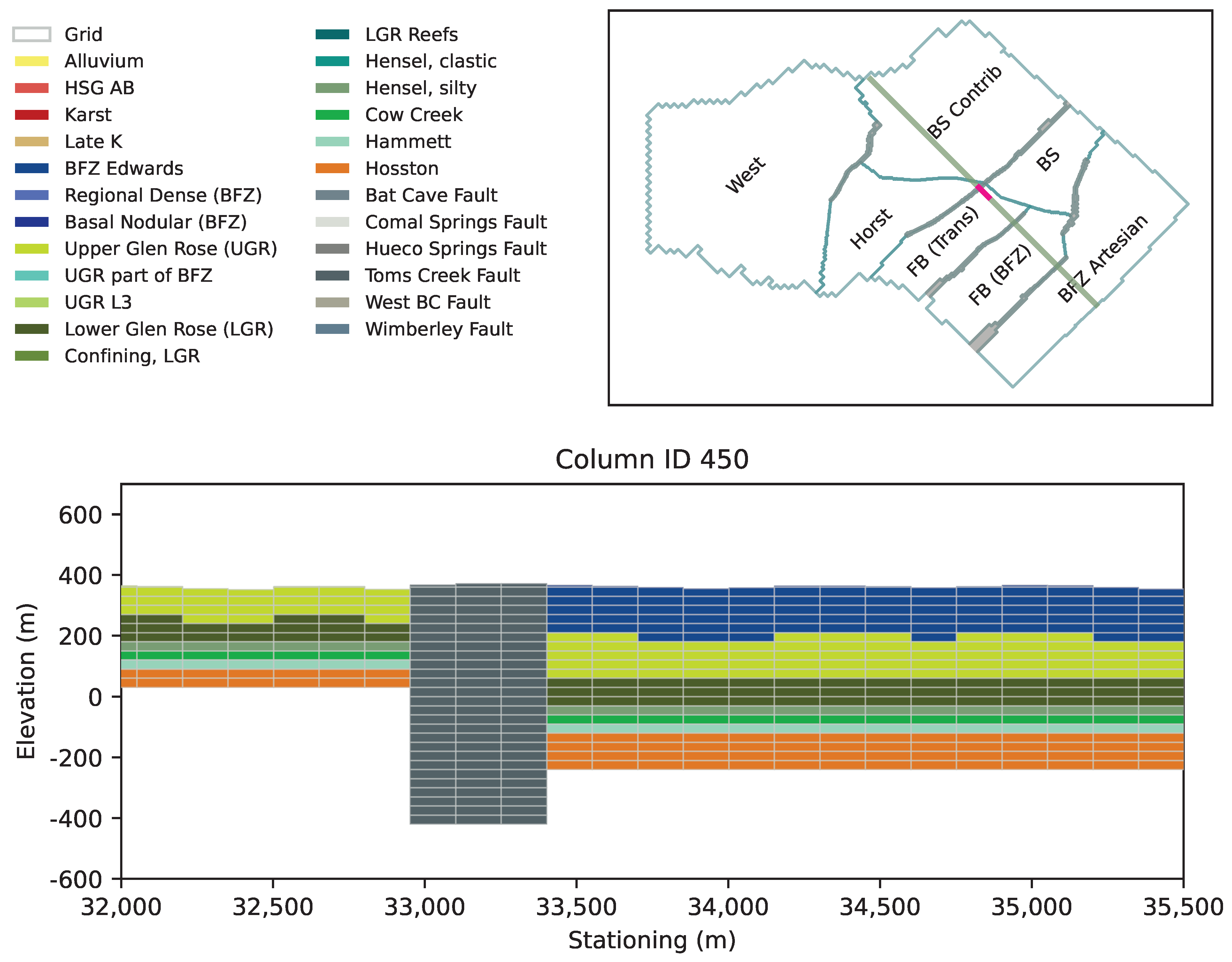
- Geostatistical interpolation within hydrostratigrapic zones for the four aquifers, see Figure 6 for pilot point (PP) locations;
- Use of the empirical relationship in Equation (A1) so that one storage parameter, instead of two, is included in optimization of parameter values.
2.4. Null Space Sensitivity Analysis
- Type I: variation in a parameter within the bounds of the prior parameter distribution, in Equation (1), causes insignificant changes in , which is the goodness-of-fit objective function for history matching with PEST++, and in model predictions employing parameters from the posterior parameter distribution, . Note that is a conditional subset of .
- Type II: variation of a parameter causes significant changes in but insignificant changes in model predictions.
- Type III: variation of a parameter causes significant changes to both and model predictions.
- Type IV: variation of a parameter causes insignificant changes to but significant changes to the model predictions.
- Parameter sensitivities are calculated by using a ratio of the description of the spread of the prior to the description of the spread of the posterior;
- Because of sampling efficiencies and the resulting limited number of realizations, the prior description should tend towards describing the largest supported spread, and the posterior description should be constrained to depict a central region;
- The null space is estimated by determining which sensitivity metric values correspond to sensitive and insensitive parameters
- This is expected to be a trial-and-error process that is site-specific, dependent on data sufficiency, and influenced by observation error models.
- An approach that we have found useful is to employ sensitivity metric quartiles as the first step in the search for the sensitive versus insensitive demarcation and then to refine to decile metric values if needed.
- Each demarcation metric percentile that is evaluated will need to be used in forward model simulation with sensitive parameters fixed to final model values and insensitive parameters set to a prior boundary value (e.g., or ) to determine whether this is an effective demarcation level. The effective demarcation level is the largest percentile sensitivity metric value that maintains model validation.
- An ensemble of sensitivity analysis models is created, leveraging the effective demarcation sensitivity metric value to fix sensitive parameters to final model values for all ensemble members and to vary insensitive parameters within the prior ranges across ensemble members;
- It is confirmed that model validation is retained for all sensitivity analysis ensemble members;
- Sensitivity analysis model simulation results are evaluated for variations to or changes in model predictions;
- Changes in model predictions then identify Type IV sensitivity.
3. Results
3.1. Validation of Assimilation
3.2. Empirical Null Space Sensitivity Analysis for Ensemble Methods
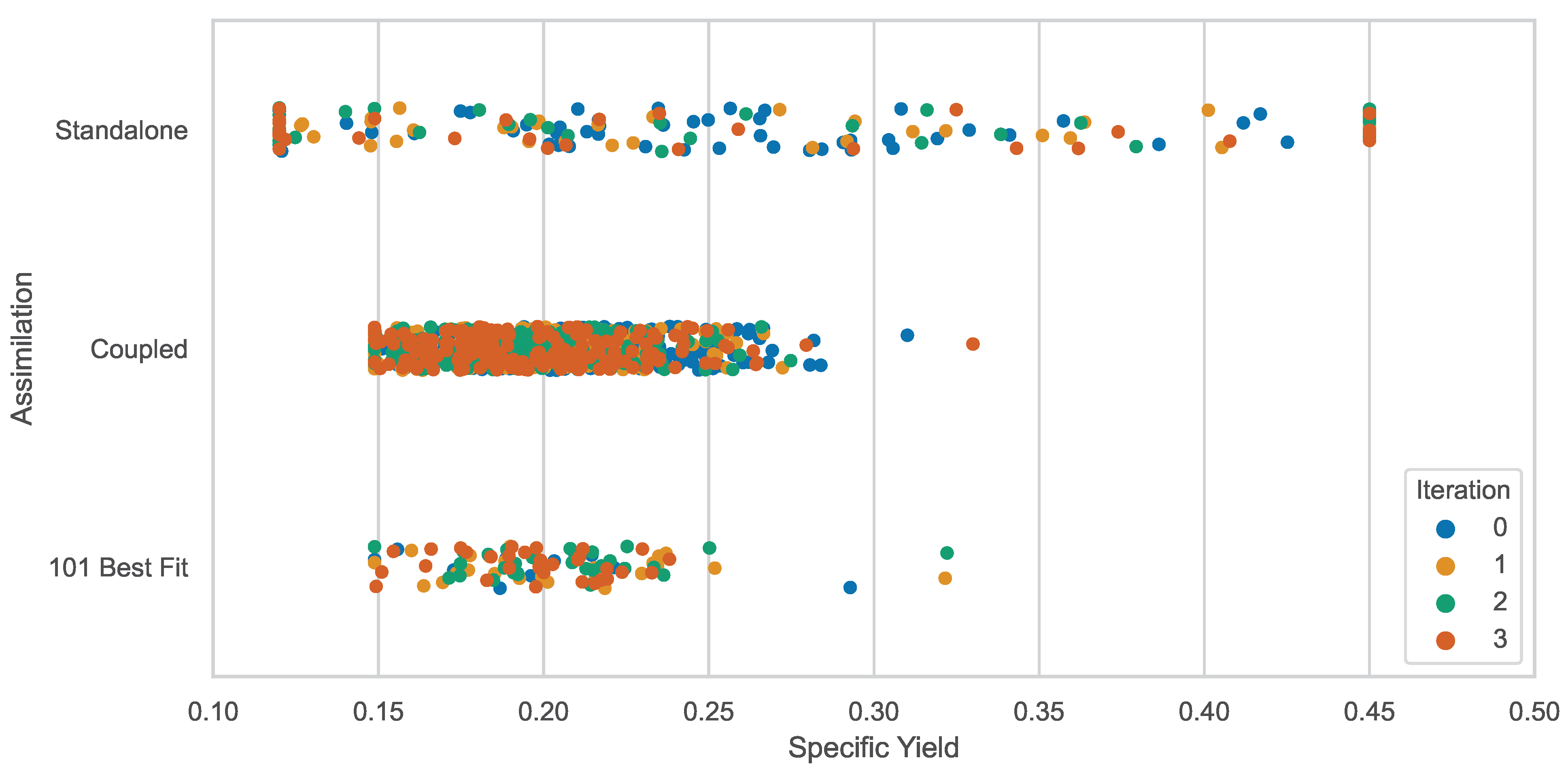
- S1, sensitivity analysis ensemble 1: set to 0.15. Hydraulic conductivity, K, values, x-, y-, and z-directions, set to .
- S2, sensitivity analysis ensemble 2: set to 0.20. K values, x-, y-, and z-directions, set to .
- S3, sensitivity analysis ensemble 3: set to 0.25. K values, x-, y-, and z-directions, set to .
- S4, sensitivity analysis ensemble 4: set to 0.30. K values, x-, y-, and z-directions, set to .
- S5, sensitivity analysis ensemble 5: set to 0.35. K values, x-, y-, and z-directions, set to .
4. Discussion
4.1. Model Complexity and Bias–Variance Tradeoff
4.2. Addressing Uncertainty from Imperfect Models and Insufficient Data
4.3. Future Work
5. Conclusions
Author Contributions
Funding
Data Availability Statement
Acknowledgments
Conflicts of Interest
Abbreviations
| ADCP | Acoustic Doppler current profiler |
| BFZ | Balcones Fault Zone |
| BRAAT | Blanco River Aquifers Assessment Tool |
| CFD | Computational fluid dynamics |
| DA | Data assimilation |
| DNS | Direct numerical simulation |
| EnKF | Ensemble Kalman filter |
| FTABLE | Volume to discharge empirical lookup table in HSPF |
| HRU | Hydrologic response unit |
| HSPF | Hydrological Simulation Program–FORTRAN |
| iES | Iterative ensemble smoother |
| Hydraulic conductivity in the x-direction | |
| Hydraulic conductivity in the y-direction | |
| Hydraulic conductivity in the z-direction | |
| MA | Monthly-averaged water level elevation |
| MCMC | Markov Chain Monte Carlo |
| NRMSE | Normalized root mean square error |
| NSE | Nash–Sutcliffe Efficiency, Equation (A3) |
| NSMC | Null Space Monte Carlo |
| ODE | Ordinary differential equation |
| PDE | Partial differential equation |
| PERLND | Pervious land segment in HSPF |
| PP | Pilot point |
| PT | Point-in-time water level elevation |
| pyHS2MF6 | Integrated hydrological model |
| RANS | Reynolds-averaged Navier–Stokes equations |
| RCHRES | Well-mixed reservoir structure in HSPF |
| RMSE | Root mean square error, Equation (A2) |
| Specific storage | |
| Specific yield | |
| TIFP | Texas Instream Flow Program |
| TRIM | Tidal, Residual, Intertidal Mudflat Model |
| TX | Texas |
| UZF | Unsaturated Zone Flow advanced stress package in MODFLOW 6 |
Appendix A
Appendix A.1. Data Availability Tables

| Data Source Name | Last Accessed |
|---|---|
| Conceptual Model Report | 28 August 2024 |
| pyHS2MF6 Source Code | 28 August 2024 |
| pyHS2MF6 Development Documentation | 28 August 2024 |
| Calibration Files and Scripts | 28 August 2024 |
| Calibrated and Validated Model Files | 28 August 2024 |
| Draft BRAAT 1 HSPF Model: Standalone Setup and Configuration | 28 August 2024 |
| Draft BRAAT 1: MODFLOW 6 Setup and Configuration Documentation | 28 August 2024 |
| Draft BRAAT 1 Phase II, Components A & B | 28 August 2024 |
| Data Source Name | Last Accessed |
|---|---|
| Water Data for Texas | 2 September 2024 |
| Web Soil Survey | 29 July 2020 |
| United States Geological Survey (USGS) Discharge Data | 13 September 2022 |
| Lower Colorado River Authority (LCRA) Discharge Data | 13 September 2022 |
| PRISM Climate Group | 28 August 2024 |
| TWDB 1 Historical Groundwater Pumpage | 28 August 2024 |
| Texas Water Rights Viewer | 28 August 2024 |
| NPDES Monitoring Data Download | 28 August 2024 |
| Data Source Name | Last Accessed |
|---|---|
| Edwards Aquifer Authority (EAA) | 2 September 2024 |
| Barton Springs Edwards Aquifer Conservation District (BSEACD) | 2 September 2024 |
| Blanco-Pedernales Groundwater Conservation District (BPGCD) | 2 September 2024 |
| Cow Creek Groundwater Conservation District (CCGCD) | 2 September 2024 |
| Comal Trinity Groundwater Conservation District (CTGCD) | 2 September 2024 |
| Hays Trinity Groundwater Conservation District (HTGCD) | 2 September 2024 |
| Hill Country Underground Water Conservation District (HCUWCD) | 2 September 2024 |
| Southwestern Travis County Groundwater Conservation District (SWTCGCD) | 2 September 2024 |
Appendix A.2. Blanco River Aquifers Assessment Tool (BRAAT) Project
| Id 1 | Descriptive Label | Short Label 2 |
|---|---|---|
| 1 | Balcones Fault Zone (BFZ) Edwards Artesian Region | BFZ Artesian |
| 2 | BFZ Edwards Fault Blocks Region | BFZ FBlocks |
| 3 | Barton Springs Pool Region | Barton Springs |
| 4 | Transition Fault Blocks Region | Trans FBlocks |
| 5 | Barton Springs Contributing Area Region | BS Contrib |
| 6 | Horst Block and Southern Wedge Region | Horst South |
| 7 | Far West Region | West |
| 8 3 | Bounding Fault Zones Region | Fault Zones |
Appendix A.2.1. Observations
Appendix A.2.2. Integrated Hydrological Model Development
Appendix A.2.3. Integrated Hydrological Model Implementation
| Model | Parameter | Number Adjusted | Notes |
|---|---|---|---|
| HSPF | FTABLE 1 discharge magnitudes for focused range of volume indices | 409 | There are two exits or ports from each of the 24 RCHRES 2 that have a volume dependent solution and use the FTABLES. The “lower” volume table indices, generally corresponding to a stage of 1.5 to 10.0 ft, were adjusted as part of coupled model calibration. |
| UZF | Vertical, saturated hydraulic conductivity vks, which is similar to | 92 | UZF assumes vertical porous media flow using a method of characteristics solution. Parameterization is zone-based for regionalization with zones identified from HSPF RCHRES 2 or PERLND 3 footprints. Gross adjustment range was 1.1 to 500.0 m/d. |
| UZF | Saturated water content, thts, which is similar to | 92 | UZF assumes vertical porous media flow using a method of characteristics solution. Parameterization is zone-based for regionalization with zones identified from HSPF RCHRES 2 or PERLND 3 footprints. Gross adjustment range was 0.10 to 0.35. |
| Parameter | Number Adjusted | Notes |
|---|---|---|
| DRN 1 Conductance | 17 | DRNs represent designated springs. One conductance value is applied to all DRN cells that represent a particular spring. |
| Zone-based hydraulic conductivity in x-direction, | 121 | Varies by water budget unit. Gross overall range is 0.04 to 100.0 m/d. |
| Zone-based hydraulic conductivity in y-direction, | 121 | Varies by water budget unit. Gross overall range is 0.04 to 100.0 m/d. |
| Zone-based hydraulic conductivity in z-direction, | 99 | Some important confining water budget units have z–direction pilot points and zone-based values for x- and y-direction and specific yield. Varies by water budget unit. Gross overall range is 0.01 to 42.0 m/d. |
| Zone-based specific yield, | 121 | Varies by water budget unit. Gross overall range is 0.10 to 0.36. Specific storage, , calculated from using Equation (A1). |
| Pilot points (PP) hydraulic conductivity in x-direction, | 875 | Varies by water budget unit. Gross overall range is 0.8 to 141.5 m/d. |
| Pilot points (PP) hydraulic conductivity in y-direction, | 875 | Varies by water budget unit. Gross overall range is 0.8 to 141.5 m/d. |
| Pilot points (PP) hydraulic conductivity in z-direction, | 1642 | Some important confining water budget units have z–direction pilot points and zone-based values for x- and y-direction and specific yield. Varies by water budget unit. Gross overall range is 0.007 to 55.0 m/d. |
| Pilot points (PP) specific yield, | 875 | Varies by water budget unit. Gross overall range is 0.10 to 0.45. Specific storage, , calculated from using Equation (A1). |
| Parameter Name | Structure Type | Definition | Range 1 | |
|---|---|---|---|---|
| Max 2 | Min 2 | |||
| LZSN | PERLND 3 | Lower zone nominal soil moisture storage in inches | 9.0 | 3.0 |
| INFILT | PERLND 3 | Index to infiltration capacity, in/hr | 0.4 | 0.001 |
| AGWRC | PERLND 3 | Base groundwater recession | 0.999 | 0.85 |
| DEEPFR | PERLND 3 | Fraction of groundwater inflow to “deep recharge” 4 | 0.9 | 0.0 |
| UZSN | PERLND 3 | Upper zone nominal soil moisture storage in inches | 2.0 | 0.05 |
| INTFW | PERLND 3 | Interflow inflow parameter | 10.0 | 0.58 |
| IRC | PERLND 3 | Interflow recession parameter | 0.85 | 0.3 |
| RETSC | IMPLND 5 | Retention storage capacity in inches | 0.3 | 0.01 |


| Color Key 1 | ID | Name | Type | Purpose |
|---|---|---|---|---|
| ine | 1 | Alluvium | transition | At and near surface transition to groundwater |
| 2 | HSG AB 2 | transition | At and near surface transition to groundwater | |
| 5 | Karst | transition | At and near surface transition to groundwater | |
| 6 | Karst Transition | transition | At and near surface transition to groundwater | |
| 11 | Late K Confining | confining | Surficial deposits east and south of BFZ | |
| 21 | Plateau Edwards | NA | Minimal footprint and only in far west | |
| 31 | BFZ Edwards | primary aquifer | BFZ Edwards Aquifer | |
| 32 | Regional Dense (BFZ Edwards) | confining | Internal separation of BFZ Edwards | |
| 33 | Basal Nodular (BFZ Edwards) | confining | Separation from Upper Trinity Aquifer | |
| 41 | Upper Glen Rose (UGR) | aquifer | Upper Trinity Aquifer | |
| 42 | Upper Glen Rose, part of BFZ Edwards Aquifer | aquifer | BFZ Edwards Aquifer | |
| 43 | Lower Aquitard, Unit 3 (UGR) | confining | Separation from Lower Glen Rose | |
| 46 | Lower Glen Rose (LGR) | aquifer | part of Middle Trinity Aquifer | |
| 47 | Upper Aquitard (LGR) | confining | Internal separation from Cow Creek | |
| 48 | Reef Facies (LGR) | aquifer | part of Middle Trinity Aquifer [56] | |
| 51 | Hensel siliclastic facies | aquifer | Part of Middle Trinity Aquifer in the western part of the domain [69] | |
| 52 | Hensel, thin silty facies | confining | Separation of LGR and Reef Facies from Cow Creek [69] | |
| 56 | Cow Creek | aquifer | Most productive part of Middle Trinity Aquifer | |
| 61 | Hammett | confining | Separation between Middle and Lower Trinity Aquifers | |
| 71 | Sycamore or Hosston | aquifer | Lower Trinity Aquifer | |
| 81 | Undifferentiated Paleozoic | NA | Minor instances in the north near Pedernales River |
| Color Key 1 | Water Budget Unit ID 2 | Hydrostratigraphy IDs 3 | Description | Regionalization Method 4 |
|---|---|---|---|---|
| ine | X0001 | 1 | Alluvium | zone for all |
| X0002 | 2 | HSG AB | zone for all | |
| X0005 | 5, 6 | Karst | zone for all | |
| X0011 | 11 | Late K Confining | zone for all | |
| X0021 | 21 | Plateau Edwards | zone for all | |
| X0031 | 31, 42 | BFZ Edwards Aquifer | PP for all | |
| X0032 | 32, 33 | Confining within BFZ Edwards | PP for ; zone for , , and | |
| X0041 | 41 | Upper Trinity Aquifer | PP for ; zone for , , and | |
| X0042 | 43 | Upper Glen Rose (UGR), confining | PP for ; zone for , , and | |
| X0051 | 46, 48 | Lower Glen Rose (LGR), Middle Trinity Aquifer | PP for all | |
| X0052 | 47 | Lower Glen Rose (LGR), confining | PP for ; zone for , , and | |
| X0053 | 56, 51 | Cow Creek, Middle Trinity Aquifer | PP for all | |
| X0054 | 52 | Hensel, confining | zone for all | |
| X0061 | 61 | Hammett, confining | PP for ; zone for , , and | |
| X0071 | 71 | Lower Trinity Aquifer | PP for all | |
| X0081 | 81 | Undifferentiated Paleozoic | zone for all |
Appendix A.2.4. Integrated Hydrological Model Validation
- Simulation and Burn-in Start: 2015–01–01
- Burn-in End: 2016–06–30 (1.5 years of burn-in)
- History Matching Start: 2016–07–01
- History Matching End: 2019–12–31 (3.5 years of calibration)
- Validation Start: 2020–01–01
- Validation and Simulation End: 2021–12–31 (2.0 years of validation; 7.0 years of simulation)
References
- Evensen, G.; Vossepoel, F.; Jan van Leeuwen, P. Data Assimilation Fundamentals: A Unified Formulation of the State and Parameter Estimation Problem; Springer: Cham, Switzerland, 2022. [Google Scholar]
- White, J.T. A model-independent iterative ensemble smoother for efficient history-matching and uncertainty quantification in very high dimensions. Environ. Model. Softw. 2018, 109, 191–201. [Google Scholar] [CrossRef]
- Tonkin, M.; Doherty, J. Calibration-constrained Monte Carlo analysis of highly parameterized models using subspace techniques. Water Resour. Res. 2009, 45, W00B10. [Google Scholar] [CrossRef]
- Doherty, J. Calibration and Uncertainty Analysis for Complex Environmental Models. PEST: Complete Theory and What It Means for Modelling the Real World; Watermark Numerical Computing: Brisbane, Australia, 2015. [Google Scholar]
- Alstad, V.; Skogestad, S. Null Space Method for Selecting Optimal Measurement Combinations as Controlled Variables. Ind. Eng. Chem. Res. 2007, 46, 846–853. [Google Scholar] [CrossRef]
- Zeng, G.L.; Gullberg, G.T. Null-Space Function Estimation for the Interior Problem. Phys. Med. Biol. 2012, 57, 1873–1887. [Google Scholar] [CrossRef]
- Herckenrath, D.; Langevin, C.D.; Doherty, J. Predictive uncertainty analysis of a saltwater intrusion model using null-space Monte Carlo. Water Resour. Res. 2011, 47, 47. [Google Scholar] [CrossRef]
- Yoon, H.; Hart, D.B.; McKenna, S.A. Parameter estimation and predictive uncertainty in stochastic inverse modeling of groundwater flow: Comparing null-space Monte Carlo and multiple starting point methods. Water Resour. Res. 2013, 49, 536–553. [Google Scholar] [CrossRef]
- Tavakoli, R.; Yoon, H.; Delshad, M.; ElSheikh, A.H.; Wheeler, M.F.; Arnold, B.W. Comparison of ensemble filtering algorithms and null-space Monte Carlo for parameter estimation and uncertainty quantification using CO2 sequestration data. Water Resour. Res. 2013, 49, 8108–8127. [Google Scholar] [CrossRef]
- Colombo, L.; Alberti, L.; Mazzon, P.; Antelmi, M. Null-Space Monte Carlo Particle Backtracking to Identify Groundwater Tetrachloroethylene Sources. Front. Environ. Sci. 2020, 8, 142. [Google Scholar] [CrossRef]
- Moeck, C.; Molson, J.; Schirmer, M. Pathline Density Distributions in a Null-Space Monte Carlo Approach to Assess Groundwater Pathways. Groundwater 2020, 58, 189–207. [Google Scholar] [CrossRef]
- Saad, S.; Javadi, A.A.; Farmani, R.; Sherif, M. Efficient uncertainty quantification for seawater intrusion prediction using Optimized sampling and Null Space Monte Carlo method. J. Hydrol. 2023, 620, 129496. [Google Scholar] [CrossRef]
- Baalousha, H.M. Predictive uncertainty analysis for a highly parameterized karst aquifer using null-space Monte Carlo. Front. Water 2024, 6, 1384983. [Google Scholar] [CrossRef]
- Moges, E.; Demissie, Y.; Li, H. Uncertainty propagation in coupled hydrological models using winding stairs and null-space Monte Carlo methods. J. Hydrol. 2020, 589, 125341. [Google Scholar] [CrossRef]
- Hewett, R.J.; Heath, M.T.; Butala, M.D.; Kamalabadi, F. A Robust Null Space Method for Linear Equality Constrained State Estimation. IEEE Trans. Signal Process. 2010, 58, 3961–3971. [Google Scholar] [CrossRef]
- Yang, Y.; Maley, J.; Huang, G. Null-space-based marginalization: Analysis and algorithm. In Proceedings of the 2017 IEEE/RSJ International Conference on Intelligent Robots and Systems (IROS), Vancouver, BC, Canada, 24–28 September 2017; pp. 6749–6755, ISSN 2153-0866. [Google Scholar] [CrossRef]
- Martin, N.; Green, R.T.; Nicholaides, K.; Fratesi, S.B.; Nunu, R.R.; Flores, M.E. Blanco River Aquifer Assessment Tool—A Tool to Assess How the Blanco River Interacts with Its Aquifers: Creating the Conceptual Model; Technical Report; Meadows Center for Water and the Environment, Texas State University: San Marcos, TX, USA, 2019. [Google Scholar]
- TWDB. Texas Instream Flow Program, 2024. Available online: https://www.twdb.texas.gov/surfacewater/flows/instream/index.asp (accessed on 11 June 2024).
- Martin, N.; White, J. Flow Regime-Dependent, Discharge Uncertainty Envelope for Uncertainty Analysis with Ensemble Methods. Water 2023, 15, 1133. [Google Scholar] [CrossRef]
- McMillan, H.; Krueger, T.; Freer, J. Benchmarking observational uncertainties for hydrology: Rainfall, river discharge and water quality. Hydrol. Process. 2012, 26, 4078–4111. [Google Scholar] [CrossRef]
- Slade, R.M. A recharge-discharge water budget and evaluation of water budgets for the Edwards Aquifer associated with Barton Springs. Tex. Water J. 2017, 8, 42–56. [Google Scholar] [CrossRef]
- Slade, R.M. Documentation of a recharge-discharge water budget and main-streambed recharge volumes, and fundamental evaluation of groundwater tracer studies for the Barton Springs segment of the Edwards Aquifer. Tex. Water J. 2014, 5, 12–23. [Google Scholar] [CrossRef]
- HDR Engineering, Inc.; Paul Price Associates, Inc.; LBG-Guyton Associates; Fugro-McClelland (SW), Inc. Trans-Texas Water Program, West Central Study Area Phase II: Edwards Aquifer Recharge Analyses; Technical Report; San Antonio River Authority and Others: San Antonio, TX, USA, 1998. [Google Scholar]
- Puente, C. Method of Estimating Natural Recharge to the Edwards Aquifer in the San Antonio Area, Texas; Water-Resources Investigation Report 78-0010; U.S Geological Survey: Austin, TX, USA, 1978.
- Orszag, S.A. Analytical theories of turbulence. J. Fluid Mech. 1970, 41, 363–386. [Google Scholar] [CrossRef]
- Ciofalo, M. Direct Numerical Simulation (DNS). In Thermofluid Dynamics of Turbulent Flows: Fundamentals and Modelling; Ciofalo, M., Ed.; UNIPA Springer Series; Springer International Publishing: Cham, Switzerland, 2022; pp. 37–46. [Google Scholar] [CrossRef]
- Jungbecker, P.; Veit, D. Computational fluid dynamics (CFD) and its application to textile technology. In Simulation in Textile Technology; Veit, D., Ed.; Woodhead Publishing Series in Textiles; Woodhead Publishing: Sawston, UK, 2012; pp. 142–171, 172e–178e. [Google Scholar] [CrossRef]
- Roelofs, F.; Shams, A. CFD—Introduction. In Thermal Hydraulics Aspects of Liquid Metal Cooled Nuclear Reactors; Roelofs, F., Ed.; Woodhead Publishing: Sawston, UK, 2019; pp. 213–218. [Google Scholar] [CrossRef]
- Casulli, V.; Cattani, E. Stability, accuracy and efficiency of a semi-implicit method for three-dimensional shallow water flow. Comput. Math. Appl. 1994, 27, 99–112. [Google Scholar] [CrossRef]
- Casulli, V.; Cheng, R.T. Semi-implicit finite difference methods for three-dimensional shallow water flow. Int. J. Numer. Methods Fluids 1992, 15, 629–648. [Google Scholar] [CrossRef]
- Chow, V.T.; Maidment, D.R.; Mays, L.W. Applied Hydrology; McGraw-Hill Education: New York, NY, USA, 1988. [Google Scholar]
- US EPA. BASINS Technical Note 6: Estimating Hydrology and Hydraulic Parameters for HSPF; Technical Note EPA-823-R00-012; US EPA: Washington, DC, USA, 2000.
- Langevin, C.D.; Hughes, J.D.; Banta, E.R.; Provost, A.M.; Niswonger, R.G.; Panday, S. MODFLOW 6 Modular Hydrologic Model Version 6.1.1; U.S. Geological Survey: Reston, VA, USA, 2019. [CrossRef]
- U.S. Geological Survey. MODFLOW 6: USGS Modular Hydrologic Model; U.S. Geological Survey: Reston, VA, USA, 2020.
- Freeze, A.R.; Cherry, J.M. Groundwater; Pearson: London, UK, 1979. [Google Scholar]
- Bear, J. Dynamics of Fluids in Porous Media, Unabridged Reprint ed.; Dover Science Books, Dover Publications, Inc.: New York, NY, USA, 1988; Original Publication: 1972 American Elsevier Publishing Company, Inc. [Google Scholar]
- Pest++ Development Team. PEST++: Software Suite for Parameter Estimation, Uncertainty Quantification, Management Optimization, and Sensitivity Analysis. Version 5.1.18. User Manual. Pest++ Development Team. [Online]. 2022. Available online: https://github.com/usgs/pestpp (accessed on 26 June 2024).
- White, J.T.; Hunt, R.J.; Fienen, M.N.; Doherty, J. Approaches to Highly Parameterized Inversion: PEST++ Version 5, a Software Suite for Parameter Estimation, Uncertainty Analysis, Management Optimization and Sensitivity Analysis; Techniques and Methods 7C26; U.S. Geological Survey: Reston, VA, USA, 2020.
- Chen, Y.; Oliver, D.S. Levenberg–Marquardt forms of the iterative ensemble smoother for efficient history matching and uncertainty quantification. Comput. Geosci. 2013, 17, 689–703. [Google Scholar] [CrossRef]
- Doherty, J. PEST Model-Independent Parameter Estimation, User Manual Part I: PEST, SENSAN and Global Optimisers, User Manual 7th ed.; Watermark Numerical Computing: Brisbane, Australia, 2020. [Google Scholar]
- Evans, M.; Moshonov, H. Checking for prior-data conflict. Bayesian Anal. 2006, 1, 893–914. [Google Scholar] [CrossRef]
- Alfonzo, M.; Oliver, D.S. Evaluating prior predictions of production and seismic data. Comput. Geosci. 2019, 23, 1331–1347. [Google Scholar] [CrossRef]
- Oliver, D.S. Diagnosing reservoir model deficiency for model improvement. J. Pet. Sci. Eng. 2020, 193, 107367. [Google Scholar] [CrossRef]
- Hastie, T.; Tibshirani, R.; Friedman, J. The Elements of Statistical Learning: Data Mining, Inference, and Prediction, 2nd ed.; Springer Science+Business Media: New York, NY, USA, 2016. [Google Scholar] [CrossRef]
- Chollet, F. Deep Learning with Python, 2nd ed.; Manning Publications Company: Shelter Island, NY, USA, 2021. [Google Scholar]
- Martin, N.; White, J. Water Resources’ AI–ML Data Uncertainty Risk and Mitigation Using Data Assimilation. Water 2024, 16, 2758. [Google Scholar] [CrossRef]
- ASTM International. Standard Guide for Conducting a Sensitivity Analysis for a Groundwater Flow Model Application; ASTM International: West Conshohocken, PA, USA, 2016. [Google Scholar]
- Nash, J.E.; Sutcliffe, J.V. River flow forecasting through conceptual models part I—A discussion of principles. J. Hydrol. 1970, 10, 282–290. [Google Scholar] [CrossRef]
- Legates, D.R.; McCabe, G.J. Evaluating the use of “goodness-of-fit” measures in hydrologic and hydroclimatic model validation. Water Resour. Res. 1999, 35, 233–241. [Google Scholar] [CrossRef]
- Anderson, M.P.; Woessner, W.W. Applied Groundwater Modeling: Simulation of Flow and Advective Transport, 1st ed.; Academic Press: San Diego, CA, USA, 1991. [Google Scholar]
- Martin, N. Watershed-Scale, Probabilistic Risk Assessment of Water Resources Impacts from Climate Change. Water 2021, 13, 40. [Google Scholar] [CrossRef]
- Martin, N. Risk Assessment of Future Climate and Land Use/Land Cover Change Impacts on Water Resources. Hydrology 2021, 8, 38. [Google Scholar] [CrossRef]
- Karniadakis, G.E.; Kevrekidis, I.G.; Lu, L.; Perdikaris, P.; Wang, S.; Yang, L. Physics-informed machine learning. Nat. Rev. Phys. 2021, 3, 422–440. [Google Scholar] [CrossRef]
- Delottier, H.; Doherty, J.; Brunner, P. Data space inversion for efficient uncertainty quantification using an integrated surface and sub-surface hydrologic model. Geosci. Model Dev. 2023, 16, 4213–4231. [Google Scholar] [CrossRef]
- Bala, B.K.; Arshad, F.M.; Noh, K.M. System Dynamics: Modelling and Simulation; Springer Texts in Business and Economics; Springer: Singapore, 2017. [Google Scholar]
- Wierman, D.; Broun, A.; Hunt, B. Hydrogeologic Atlas of the Hill Country Trinity Aquifer: Blanco, Hays, and Travis Counties, Central Texas; Hydrogeologic Atlas; The Meadows Center for Water and the Environment—Texas State University: San Marcos, TX, USA, 2010. [Google Scholar]
- Hunt, B.; Smith, B.; Andrews, A.; Wierman, D.; Broun, A.; Gary, M. Relay Ramp Structures and their Influence on Groundwater Flow in the Edwards and Trinity Aquifers, Hays and Travis Counties, Central Texas. In Proceedings of the 14th Multidisciplinary Conference on Sinkholes and the Engineering and Environmental Impacts of Karst, Carlsbad, NM, USA, 5–9 October 2015; pp. 189–200. [Google Scholar]
- Hunt, B.B.; Smith, B.A.; Gary, M.O.; Broun, A.S.; Wierman, D.A.; Watson, J.; Johns, D. Surface-water and Groundwater Interactions in the Blanco River and Onion Creek Watersheds: Implications for the Trinity and Edwards Aquifers of Central Texas. Bull. South Tex. Geol. Soc. 2017, 47, 33–53. [Google Scholar]
- Smith, B.A.; Hunt, B.B.; Wierman, D.A.; Gary, M.O. Groundwater Flow Systems in Multiple Karst Aquifers of Central Texas. In Proceedings of the 15th Multidisciplinary Conference on Sinkholes and the Engineering and Environmental Impacts of Karst: National Cave and Karst Research Institute (NCKRI), Carlsbad, NM, USA, 2–6 April 2018; pp. 17–29. [Google Scholar]
- Clark, A.K.; Golab, J.A.; Morris, R.E. Geologic Framework, Hydrostratigraphy, and Ichnology of the Blanco, Payton, and Rough Hollow 7.5-Minute Quadrangles, Blanco, Comal, Hays, and Kendall Counties, Texas; USGS Numbered Series 3363; U.S. Geological Survey: Reston, VA, USA, 2016.
- Clark, A.K.; Golab, J.A.; Morris, R.R. Geologic Framework and Hydrostratigraphy of the Edwards and Trinity Aquifers Within Northern Bexar and Comal Counties, Texas; USGS Numbered Series 3366; U.S. Geological Survey: Reston, VA, USA, 2016.
- Clark, A.K.; Morris, R.R. Bedrock Geology and Hydrostratigraphy of the Edwards and Trinity Aquifers Within the Driftwood and Wimberley 7.5-Minute Quadrangles, Hays and Comal Counties, Texas; USGS Numbered Series 3386; U.S. Geological Survey: Reston, VA, USA, 2017.
- Clark, A.K.; Pedraza, D.E.; Morris, R.R. Geologic Framework and Hydrostratigraphy of the Edwards and Trinity Aquifers Within Hays County, Texas; USGS Numbered Series 3418; U.S. Geological Survey: Reston, VA, USA, 2018.
- Collins, E.; Hvorka, S. Structure Map of the San Antonio Segment of the Edwards Aquifer; Miscellaneous Map No. 38; University of Texas Bureau of Economic Geology (BEG): Austin, TX, USA, 1997. [Google Scholar]
- Ferrill, D.A.; Morris, A.P.; McGinnis, R.N. Geologic structure of the Edwards (Balcones Fault Zone) Aquifer. In The Edwards Aquifer: The Past, Present, and Future of a Vital Water Resource; GSA Memoirs; Sharp, J.M., Jr., Green, R.T., Schindel, G.M., Eds.; Geological Society of America: Boulder, CO, USA, 2019; Volume 215, p. 18. [Google Scholar] [CrossRef]
- Ferguson, W. The Blanco River; Texas A&M University Press: College Station, TX, USA, 2017. [Google Scholar]
- Martin, N. pyHS2MF6 Docs. 2021. Available online: https://nmartin198.github.io/pyHS2MF6/ (accessed on 2 March 2025).
- TexasWater Development Board; U.S. Geological Survey. Geologic Atlas of Texas; Bureau of Economic Geology (BEG): Austin, TX, USA, 2007. Available online: https://www.twdb.texas.gov/groundwater/aquifer/GAT/ (accessed on 27 April 2025).
- Broun, A.S.; Hunt, B.B.; Watson, J.A.; Wierman, D.A. A Reevaluation of the Lithostratigraphy and Facies of the Lower Cretaceous Hensel Sand–Lower Glen Rose Transitions, Comanchean Shelf, Blanco and Hays Counties, Central Texas. GCAGS J. 2020, 9, 76–92. [Google Scholar]
- Soil Survey Staff, Natural Resources Conservation Service, United States Department of Agriculture. Web Soil Survey, 2019. Available online: https://websoilsurvey.nrcs.usda.gov/app/ (accessed on 14 April 2021).
- Natural Resources Conservation Service (NRCS). Hydrologic Soil Groups. In National Engineering Handbook (NEH) Part 630, Hydrology; U.S. Department of Agriculture: Washington, DC, USA, 2007; p. 14. [Google Scholar]


| Goodness-of-Fit Metric | Metric Value | Validation Range | ||
|---|---|---|---|---|
| Minimum | Maximum | |||
| NRMSE 1 | 5.8% | 0% | 10% | |
| NSE 2 | 4595 | 0.6 | 0.6 | 0.8 |
| 7817 | 0.2 | —0.9 | 0.5 | |
| 8155200 | 0.8 3 | 0.6 | 0.7 | |
| 8158700 | 0.7 | 0.6 | 0.7 | |
| 8158810 | 0.7 3 | 0.5 | 0.6 | |
| 8158813 | 0.3 | —0.3 | 0.3 | |
| 8158827 | 0.7 | 0.6 | 0.8 | |
| 8170500 | 0.4 3 | —6.4 | —4.3 | |
| 8170890 | 0.1 4 | 0.7 | 0.8 | |
| 8170950 | 0.5 | 0.1 | 0.6 | |
| 8170990 | 0.6 | 0.3 | 0.4 | |
| 8171000 | 0.6 | 0.6 | 0.7 | |
| 8171290 | 0.7 3 | —0.2 | 0.3 | |
| 8171300 | 0.6 | 0.6 | 0.8 | |
| 8171350 | 0.5 | 0.3 | 0.9 | |
| 8171400 | 0.3 3 | —0.9 | 0.2 | |
| Total Major Springs 5 | 1.5 | 1.0 6 | 1.9 6 | |
| Total Major Focus Springs 7 | 1.2 3 | 0.3 6 | 1.0 6 | |
| Total All Gauging Stations | 8.2 | 4.0 6 | 10.3 6 | |
| Goodness-of-Fit | Final 1 | S1 | S2 | S3 | S4 | S5 | |
|---|---|---|---|---|---|---|---|
| NRMSE ine | All Well Water Elevations | 5.8% | 5.8% | 5.8% | 5.8% | 5.8% | 5.8% |
| NSE | 4595 | 0.6 | 0.6 | 0.6 | 0.6 | 0.6 | 0.6 |
| 7817 | 0.2 | 0.2 | 0.2 | 0.2 | 0.2 | 0.2 | |
| 8155200 | 0.8 | 0.8 | 0.8 | 0.8 | 0.8 | 0.8 | |
| 8158700 | 0.7 | 0.7 | 0.7 | 0.7 | 0.7 | 0.7 | |
| 8158810 | 0.7 | 0.7 | 0.7 | 0.7 | 0.7 | 0.7 | |
| 8158813 | 0.3 | 0.3 | 0.3 | 0.3 | 0.3 | 0.3 | |
| 8158827 | 0.7 | 0.7 | 0.7 | 0.7 | 0.7 | 0.7 | |
| 8170500 | 0.4 | 0.3 | 0.4 | 0.4 | 0.4 | 0.4 | |
| 8170890 | 0.1 | 0.1 | 0.1 | 0.1 | 0.1 | 0.1 | |
| 8170950 | 0.5 | 0.6 | 0.5 | 0.5 | 0.5 | 0.6 | |
| 8170990 | 0.6 | 0.6 | 0.6 | 0.6 | 0.6 | 0.6 | |
| 8171000 | 0.6 | 0.7 | 0.6 | 0.6 | 0.6 | 0.6 | |
| 8171290 | 0.7 | 0.7 | 0.7 | 0.7 | 0.7 | 0.7 | |
| 8171300 | 0.6 | 0.6 | 0.6 | 0.6 | 0.6 | 0.6 | |
| 8171350 | 0.5 | 0.5 | 0.5 | 0.5 | 0.5 | 0.5 | |
| 8171400 | 0.3 | 0.3 | 0.3 | 0.3 | 0.3 | 0.4 | |
| Total Major Springs 2 | 1.5 | 1.6 | 1.5 | 1.5 | 1.5 | 1.6 | |
| Total All Gauging Stations | 8.2 | 8.4 | 8.2 | 8.2 | 8.3 | 8.3 | |
| Model Prediction | Final 1 | S1 | S2 | S3 | S4 | S5 | |
|---|---|---|---|---|---|---|---|
| Average Simulated Water Storage Volume during 2020 in Middle Trinity Aquifer, excluding Cow Creek | Water Budget Region #4 Storage (Mm3) | 6344 | 4782 | 6032 | 7237 | 8410 | 9557 |
| Water Budget Region #4 residence time multiplier 2 | 1.33 | 1.00 | 1.26 | 1.51 | 1.76 | 2.00 | |
| Water Budget Region #5 Storage (Mm3) | 8802 | 7139 | 8767 | 10,321 | 11,820 | 13,278 | |
| Water Budget Region #5 residence time multiplier 2 | 1.23 | 1.00 | 1.23 | 1.45 | 1.66 | 1.86 | |
| Water Budget Region #6 Storage (Mm3) | 7575 | 6675 | 7722 | 8720 | 9675 | 10,595 | |
| Water Budget Region #6 residence time multiplier 2 | 1.13 | 1.00 | 1.16 | 1.31 | 1.45 | 1.59 | |
| Average Simulated Water Storage Volume during 2020 in Cow Creek | Water Budget Region #4 Storage (Mm3) | 2583 | 1731 | 2058 | 2367 | 2664 | 2952 |
| Water Budget Region #4 residence time multiplier 2 | 1.49 | 1.00 | 1.19 | 1.37 | 1.54 | 1.71 | |
| Water Budget Region #5 Storage (Mm3) | 9305 | 6022 | 7606 | 9150 | 10,664 | 12,155 | |
| Water Budget Region #5 residence time multiplier 2 | 1.55 | 1.00 | 1.26 | 1.52 | 1.77 | 2.02 | |
| Water Budget Region #6 Storage (Mm3) | 4235 | 2700 | 3302 | 3871 | 4417 | 4945 | |
| Water Budget Region #6 residence time multiplier 2 | 1.57 | 1.00 | 1.22 | 1.43 | 1.64 | 1.83 | |
Disclaimer/Publisher’s Note: The statements, opinions and data contained in all publications are solely those of the individual author(s) and contributor(s) and not of MDPI and/or the editor(s). MDPI and/or the editor(s) disclaim responsibility for any injury to people or property resulting from any ideas, methods, instructions or products referred to in the content. |
© 2025 by the authors. Licensee MDPI, Basel, Switzerland. This article is an open access article distributed under the terms and conditions of the Creative Commons Attribution (CC BY) license (https://creativecommons.org/licenses/by/4.0/).
Share and Cite
Martin, N.; White, J.; Southard, P. A Null Space Sensitivity Analysis for Hydrological Data Assimilation with Ensemble Methods. Hydrology 2025, 12, 106. https://doi.org/10.3390/hydrology12050106
Martin N, White J, Southard P. A Null Space Sensitivity Analysis for Hydrological Data Assimilation with Ensemble Methods. Hydrology. 2025; 12(5):106. https://doi.org/10.3390/hydrology12050106
Chicago/Turabian StyleMartin, Nick, Jeremy White, and Paul Southard. 2025. "A Null Space Sensitivity Analysis for Hydrological Data Assimilation with Ensemble Methods" Hydrology 12, no. 5: 106. https://doi.org/10.3390/hydrology12050106
APA StyleMartin, N., White, J., & Southard, P. (2025). A Null Space Sensitivity Analysis for Hydrological Data Assimilation with Ensemble Methods. Hydrology, 12(5), 106. https://doi.org/10.3390/hydrology12050106