Skill Assessment of Water Supply Outlooks in the Colorado River Basin

Abstract

Water-supply outlooks that predict the April through July (snowmelt) runoff and assist in estimating the total water-year runoff, are very important to users that rely on the major contributing watersheds of the Colorado River. This study reviewed the skill level of April through July forecasts at 28 forecast points within the Colorado River basin. All the forecasts were made after 1950, with considerable variation in time period covered. Evaluations of the forecasts were made using summary measures, correlation measures and categorical measures. The summary measure, a skill score for mean absolute error, indicated a steady increase in forecast skill through the forecast season of January to May. The width of the distribution for each monthly forecast over the 28 locations remained similar through the forecast season. The Nash-Sutcliffe score, a correlation measure, showed similar results, with the Nash-Sutcliffe median showing an increase from 0.4 to 0.8 during the forecast season. The categorical measures used a three-section partition of the April through July runoff. The Probability of Detection for low and high flows showed an increase in skill from approx. 0.4 to 0.8 during the forecast season. The same score for mid-flow years showed limited increase in skill. The low False Alarm Rate illustrated the under forecast of high-flow years. The Bias of the mid-runoff forecasts indicated over forecast early in the forecast season (January to March), with lower Bias later in the forecast season (April and May), ending the forecast season at 1.0, indicating no Bias. Forecasts for both low and high runoff were under forecast early in the season with a Bias near 0.5, improving to nearly 1.0 by the end of the forecast season. The Hit Rate measure illustrated the difficulty of mid-flow forecasts, starting at 0.5 in January and increasing to 0.75 in May due to the forecasting assumption of normal climatology for the remaining forecast period. There was no relationship between basin elevation and forecast skill, reflecting the snow vs. rain dominance in all basins.

1. Introduction

The Colorado River basin in the western United States encompasses one-fifth the area of the continental United States over seven states, with an area of 627,000 km². Snowmelt runoff from the seasonally snow-covered mountains that comprise the headwaters of watersheds within the Colorado River basin provide water to a significant area of the southwestern United States. Water managers use seasonal water-supply outlooks, which are prepared monthly during the snow accumulation and ablation periods, to effectively plan and schedule water deliveries, reservoir releases and transfers within the basin. The forecasts are prepared jointly by the Natural Resources Conservation Service (NRCS) and the National Weather Service (NWS) [1]. The basis for the forecasts is mainly the relations between snow conditions, precipitation and discharge, primarily naturalized flow in past years. This information on snowpack, and precipitation and hydrologic conditions is used to make statistical forecasts of runoff volume past the forecast point for a specified period of time. These water-supply outlooks have been prepared on some Colorado River watersheds since the 1950s. In much of the basin, the outlooks are issued from January to May and are intended to forecast runoff in the April through July period [2].

In addition to the water-supply outlooks for the Colorado River Basin, water-supply forecasts are also made on other watersheds in the western United States, including locations in California. Evaluations of the skill of these various forecasts have been made since the late 1950s on various subsets of the forecasts in the western United States. In 1958, one of the earliest comprehensive studies of forecast skill was prepared by Work and Beaumont [3]. They compared the forecast skill of NRCS and NWS forecasts and found that using snow-survey data had some advantages over using precipitation when preparing forecasts. The next year Kohler [4] produced an analysis favoring the use of precipitation. Following that work, Shafer and Huddleston [5] reviewed historical seasonal-volume forecasts based on regression techniques and found a small improvement in forecasting skill in recent years but cautioned that large improvements in skill are not to be expected in the future by refining regression techniques. Schaake and Peck [6] partitioned error in water-supply forecasts into three parts. They proposed that errors and uncertainty in forecasting arose from unknown future precipitation and temperature, data errors and uncertainty arose from difficulties in measuring inputs and outputs of the models, and errors in the models themselves produce forecast errors. They also presented analysis techniques to quantify those errors and uncertainty. Also Dracup et al. [7] examined the accuracy of hydrologic forecasts on the Colorado River in the states of Arizona, Utah and Colorado by calculating and comparing various correlation coefficients and coefficients of prediction. They found trends in the accuracy of forecasts that were attributed to the amount of precipitation and the proportion of precipitation that was snow at the forecast location.

There was an absence of skill assessments until Hartmann et al. [8] performed a regional assessment of hydrologic forecasts emphasizing the Colorado River Basin. One recommendation of the study was to make performance evaluations publicly available. Franz et al. [9] evaluated the forecasts at 14 sites on the Colorado River and determined that the Ensemble Streamflow Prediction (ESP) system, developed by the National Weather Service (NWS), performed better than climatology forecasts.

Pagano et al. [1] evaluated forecasts on 29 unregulated rivers in the western United States. The report also presented a historical review of skill assessment reports for water supply forecasts. Pagano found high skill for forecasts issued on 1 April. Forecasts made earlier in the season contained more uncertainty but were shown to still be skillful. Pagano also found that areas with wet winters and dry springs presented higher forecast improvement over the forecast season than areas with dry winters and wet springs. Pagano also found mixed changes in skill over time when comparing different areas of the study. Pagano noted that one challenge in forecast evaluation was to normalize forecast errors to allow a fair comparison between small streams and larger rivers. Pagano and his co-authors have stated that it is desirable that the evaluation measures be chosen carefully so they are understandable and relevant to forecast users.

Hartmann et al. [10] performed an assessment of water-supply outlooks in the Colorado River basin, which established a baseline for identifying improvements in hydrologic forecasts. In a following working paper, Morrill et al. [11] prepared an assessment of the strengths and weaknesses of seasonal water supply outlooks at 54 sites in the Colorado River basin using an assortment of skill measures. These measures included traditional scalar measures (e.g., correlation, root-mean square error and bias) and categorical measures (e.g., false alarm rate, threat score). They found that the examined water supply outlooks were an improvement over using average climatology. They also found that most of the forecasts were conservative, with above-average flows under predicted and below-average flows over predicted.

The questions addressed in this research are first, what is the skill of runoff forecasts in the Colorado River Basin using summary, correlation and categorical measures; and second, how do the various skill measures compare? Third, what measures are sensitive to the different input conditions, and what improvement in skill may be possible?

2. Methods and Data

2.1. Skill Measures

We introduce summary and correlation (Table 1) and categorical measures (Table 2 and Table 3) of the skill of runoff forecasts. Summary measures indicate the error in forecasts as an arithmetic difference between the forecast and the observation. The Mean Absolute Error (MAE) has dimensions and depend on the magnitude of the runoff. For the current analysis we use a skill score (SS), i.e. normalizing by the difference of each observation from the mean (Table 1). A zero skill score indicates no skill over using the historical average observation as the forecast, a negative value indicates that using the average would be better than using the forecast, and a skill score of 1 indicates perfect skill (no error in the forecast).

Table 1. Summary and correlation measures of forecast skill.

Skill Measure	Equation a
Mean Absolute Error (MAE)	$\text{MAE}=\frac{{\displaystyle \sum }\left|f_i-o_i\right|}{n}$
Mean Square Error (MSE)	$\text{MSE}=\frac{{\displaystyle \sum }{\left(f_i-o_i\right)}^2}{n}$
MAE skill score	SSMAE = 1 − MAE/MAEcl where MAEcl = $\frac{{\displaystyle \sum }\left|\overline{o}-o_i\right|}{n}$
MSE skill score b	SSMSE = 1 − MSE/MSEcl where MSEcl = $\frac{{\displaystyle \sum }{\left(\overline{o}-o_i\right)}^2}{n}$

^a Variables: o_i is the observation, $\overline{o}$ is the mean of the observations, $f_i$ is the forecast, n is the number of observations; ^b Equivalent to Nash-Sutcliffe (NS) score.

Table 1. Summary and correlation measures of forecast skill.

Skill Measure	Equation a
Mean Absolute Error (MAE)	$\text{MAE}=\frac{{\displaystyle \sum }\left|f_i-o_i\right|}{n}$
Mean Square Error (MSE)	$\text{MSE}=\frac{{\displaystyle \sum }{\left(f_i-o_i\right)}^2}{n}$
MAE skill score	SSMAE = 1 − MAE/MAEcl where MAEcl = $\frac{{\displaystyle \sum }\left|\overline{o}-o_i\right|}{n}$
MSE skill score b	SSMSE = 1 − MSE/MSEcl where MSEcl = $\frac{{\displaystyle \sum }{\left(\overline{o}-o_i\right)}^2}{n}$

^a Variables: o_i is the observation, $\overline{o}$ is the mean of the observations, $f_i$ is the forecast, n is the number of observations; ^b Equivalent to Nash-Sutcliffe (NS) score.

For a correlation measure, we used the Nash-Sutcliffe score (NS). The Nash-Sutcliffe score is one minus the ratio of the variance of the forecasts about the observation divided by the variance of the observations about their mean. As with SSMAE, a zero NS score indicates no skill over using the average, a negative value indicates that using the average would be better than using the forecast, and a skill score of 1 indicates perfect skill (no error in the forecast). As the NS score is normalized by a variance, it is dimensionless. It is also possible to use the coefficient of determination (R²) but it was not used in the analysis as it is similar to the NS and shows the same response (not shown).

Table 2. Variables for 2 × 2 contingency table.

	Observed	Not Observed
Forecast	a	b
Not forecast	c	d

Table 2. Variables for 2 × 2 contingency table.

	Observed	Not Observed
Forecast	a	b
Not forecast	c	d

Table 3. Categorical measures.

Measure	Explanation	Equation	Range
Probability of Detection (POD)	Correct forecasts divided by observations	a/(a + c)	0–1 (perfect)
False Alarm Rate (FAR)	Incorrect forecasts divided by forecasts	b/(a + b)	1–0 (perfect)
Bias	Correct and non-correct forecasts divided by observations	(a + b)/(a + c)	>1 over; and <1 under forecast
Threat Score or Critical Success Index (TS)	Correct forecasts divided by the forecasts plus non-forecast observations	a/(a + b + c)	0–1 (perfect)
Hit Rate (HR)	Correct forecasts and correct non-forecasts, divided by total forecasts and observations	(a + d)/(a + b + c + d)	0–1 (perfect)

Table 3. Categorical measures.

Measure	Explanation	Equation	Range
Probability of Detection (POD)	Correct forecasts divided by observations	a/(a + c)	0–1 (perfect)
False Alarm Rate (FAR)	Incorrect forecasts divided by forecasts	b/(a + b)	1–0 (perfect)
Bias	Correct and non-correct forecasts divided by observations	(a + b)/(a + c)	>1 over; and <1 under forecast
Threat Score or Critical Success Index (TS)	Correct forecasts divided by the forecasts plus non-forecast observations	a/(a + b + c)	0–1 (perfect)
Hit Rate (HR)	Correct forecasts and correct non-forecasts, divided by total forecasts and observations	(a + d)/(a + b + c + d)	0–1 (perfect)

Categorical measures indicate the skill of the forecast in predicting the magnitude category of the runoff, in this case low, middle and high total-runoff categories. For example, if the forecast was for flows assigned to the low-flow category, did the low flow actually occur? Historical runoff records for each forecast point were divided into 3 runoff categories, the lower 30%, the mid 40% and highest 30% of flows. A 2 × 2 contingency table was used to count the results of forecasts versus observations in each category (Table 2) and the five categorical measures were assessed (Table 3) [12]. The Probability of Detection (POD) is intuitive, being the proportion of times the event was forecast compared to the times it occurred. The False Alarm Rate (FAR) is the proportion of forecast events that failed to occur to all forecasts; and has a negative orientation, ranging from zero (perfect) to 1.0 (poor). The Bias indicates if category is over forecast (>1) or under forecast (<1). The Threat Score (TS), also known as the Critical Success Index, is similar to the HR, except that it is only for yes forecasts, i.e. the “no” forecasts are not included. The Hit Rate (HR) is intuitive, in that it credits correct “yes” and “no” forecasts equally. The POD, TS and HR all range from zero (poor) to 1.0 (perfect).

2.2. Source of Data

Forecast and observation data for 28 locations that currently forecast April to July runoff were obtained from the Colorado Basin River Forecast Center [2]. The April through July forecast period was chosen because of the historically large amount of snowmelt runoff during that time. Hydrologic information such as gage elevation, watershed area and map coordinates for each forecast point was obtained from the USGS NWIS system [13]. All the forecasts were made after 1950, and the record usually extended to 2012, but there was considerable variation in time period covered. The forecasts examined in this study were made monthly from January to May and were an estimate of the water volume to pass the forecast point during the forecast period. The actual forecast period at the various forecast locations showed considerable variation over the historical record. Many of the early forecasts were based on a forecast period from April through September. In the 1960s, forecasts were made with the beginning of the forecast period corresponding with the month of forecast. In other words, a March forecast would be March through September, and an April forecast would be April through September. Since the 1980s, most forecasts use an April through July forecast period, which corresponds with the April through July forecast period in the western Sierra Nevada of California. Data used in this study included the forecast period (April through July), month of forecast (January, February, March, April or May for this study), and forecast flow in thousand acre feet (taf) and observed flow (taf). Table 4 shows the forecasts and observations for the April through July forecast period during two years at location 25, the Yampa River at Steamboat Springs, Colorado. It is interesting to note the forecasting trends for the dry year and the following wet year.

Table 4. Example Forecasts (Flows in taf).

Year	Forecast Month	Forecast Flow	Observed Flow
2011	January	195	105.1
2011	February	180	105.1
2011	March	196	105.1
2011	April	150	105.1
2011	May	124	105.1
2012	January	335	507.2
2012	February	335	507.2
2012	March	350	507.2
2012	April	415	507.2
2012	May	495	507.2

Table 4. Example Forecasts (Flows in taf).

Year	Forecast Month	Forecast Flow	Observed Flow
2011	January	195	105.1
2011	February	180	105.1
2011	March	196	105.1
2011	April	150	105.1
2011	May	124	105.1
2012	January	335	507.2
2012	February	335	507.2
2012	March	350	507.2
2012	April	415	507.2
2012	May	495	507.2

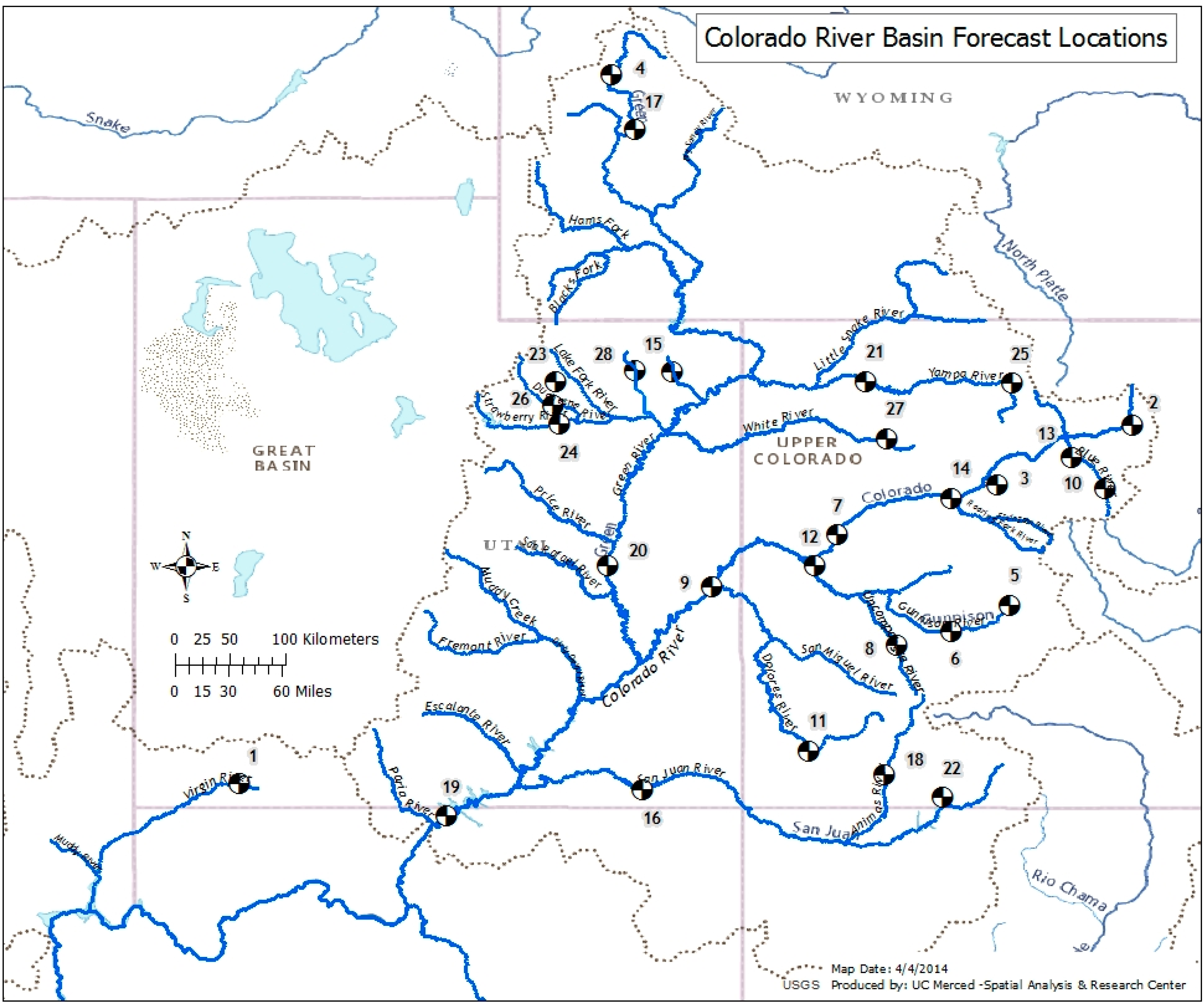
The 28 forecast locations are shown in Figure 1 along with state boundaries, a graphic delineation of watershed hydrology, and a graphic representation of topography. Details of the forecast points are shown in Table 5. Observed flows are flows that can be directly observed and are generally found in headwater basins with very few diversions and no large reservoirs that impact the natural flow [2]. Naturalized flows are calculated to estimate the unregulated flow at the measurement point, with allowance for diversions and/or reservoirs in the contributing watershed. In this dataset, 9 of the 28 points were locations with forecasts of observed flow with the remaining 19 points were locations with forecasts of naturalized flow. As expected, the locations with observed flow were on small, high-elevation watersheds with limited runoff. Once the raw data for the 28 points were tabulated and checked for consistency, the data were analyzed and skill measures calculated for the forecasts.

Figure 1. Map of the forecast points in the Colorado River basin.

Figure 1. Map of the forecast points in the Colorado River basin.

2.3. Watershed Characteristics

The elevation histogram is shown in Figure 2 along with the median watershed elevation, which ranges from 1984 m to 3364 m. The highest watershed was Blue River inflow to Dillon Reservoir, CO (#10) at 3364 m. The lowest watershed was Virgin River at Virgin, UT (#1) at 1984 m. The largest (integrating) watershed with the highest flow was Lake Powell at Glen Canyon Dam (#19) with an area of 289,303 km², and average April to July flow of 8820 million m³. The smallest watershed, which also had the smallest flow, was Ashley Creek near Vernal, UT (#15) with an area of 262 km², and an average flow of 61.4 million m³.

Table 5. Forecast point locational information.

No.	Location–Runoff Type	NWS/USGS	Lat/Lon	Runoff Records	Median Elev., m	Area, km2	Mean April–July Runoff, million m3
1	Virgin River at Virgin, UT–O	VIRU1/9406000	37.204/113.180	1958–2012	1984	2476	72
2	Colorado River below Lake Granby, CO–N	GBYC2/9019000	40.140/105.835	1954–2013	3120	808	273
3	Eagle River below Gypsum, CO–N	GPSC2/9070000	39.649/106.953	1975–2012	2971	2445	414
4	Green River at Warren Bridge, near Daniel, WY–O	WBRW4/9188500	43.019/110.119	1958–2012	2768	1212	299
5	East River at Almont, CO–N	ALEC2/9112500	38.664/106.848	1957–2012	3135	749	225
6	Gunnison River inflow to Blue Mesa Reservoir, CO–N	BMDC2/9124800	38.451/107.332	1972–2012	3023	9091	834
7	Colorado River near Cameo, CO–N	CAMC2/9095500	39.239/108.266	1957–2012	2776	20,850	2906
8	Uncompahgre River at Colona, CO–N	CLOC2/9147500	38.331/107.779	1954–2012	2807	1160	168
9	Colorado River near Cisco, UT–N	CLRU1/9180500	38.811/109.293	1957–2012	2636	62,419	5475
10	Blue River inflow to Dillon Reservoir, CO–N	DIRC2/9050700	39.626/106.066	1972–2012	3364	868	200
11	Dolores River at Dolores, CO–O	DOLC2/9166500	37.473/108.497	1954–2012	2984	1305	304
12	Gunnison River near Grand Junction, CO–N	GINC2/9152500	38.983/108.450	1954–2012	2783	20,534	1822
13	Blue River inflow to Green Mountain Reservoir, CO–N	GMRC2/9057500	39.880/106.333	1954–2012	3260	1551	339
14	Roaring Fork at Glenwood Springs, CO–N	GWSC2/9085000	39.544/107.329	1954–2012	3026	3763	853
15	Ashley Creek near Vernal, UT–O	ASHU1/9266500	40.578/109.621	1954–2012	2746	262	61
16	San Juan River near Bluff, UT–N	BFFU1/9379500	37.147/109.864	1957–2012	1985	59,570	1350
17	New Fork River near Big Piney, WY–O	BPNW4/9205000	42.567/109.929	1975–2012	2452	3186	438
18	Animas River at Durango, CO–O	DRGC2/9361500	37.279/107.880	1954–2012	3167	1792	514
19	Lake Powell at Glen Canyon Dam, AZ–N	GLDA3/9379900	36.937/111.483	1964–2012	2135	289,303	8822
20	Green River at Green River, UT–N	GRVU1/9315000	38.986/110.151	1957–2012	2135	116,162	3650
21	Yampa River near Maybell, CO–N	MBLC2/9251000	40.503/108.033	1957–2012	2316	8832	1154
22	Piedra River near Arboles, CO–O	PIDC2/9349800	37.088/107.397	1972–2012	2604	1629	258
23	Rock Creek near Mtn Home, UT–N	ROKU1/9279000	40.493/110.578	1965–2012	3121	381	109
24	Strawberry River near Duchesne, UT–N	STAU1/9288180	40.155/110.554	1954–2012	2435	2375	154
25	Yampa River at Steamboat Springs, CO–N	STMC2/9239500	40.484/106.832	1954–2012	2695	1471	318
26	Duchesne River near Tabiona, UT–N	TADU1/9277500	40.300/110.602	1954–2012	2707	914	133
27	White River near Meeker, CO–O	WRMC2/9304500	40.034/107.862	1954–2012	2763	1955	343
28	Whiterocks River near Whiterocks, UT–O	WTRU1/9299500	40.594/109.932	1954–2012	3194	282	67

Runoff Type: O = observed, N = naturalized.

Table 5. Forecast point locational information.

No.	Location–Runoff Type	NWS/USGS	Lat/Lon	Runoff Records	Median Elev., m	Area, km2	Mean April–July Runoff, million m3
1	Virgin River at Virgin, UT–O	VIRU1/9406000	37.204/113.180	1958–2012	1984	2476	72
2	Colorado River below Lake Granby, CO–N	GBYC2/9019000	40.140/105.835	1954–2013	3120	808	273
3	Eagle River below Gypsum, CO–N	GPSC2/9070000	39.649/106.953	1975–2012	2971	2445	414
4	Green River at Warren Bridge, near Daniel, WY–O	WBRW4/9188500	43.019/110.119	1958–2012	2768	1212	299
5	East River at Almont, CO–N	ALEC2/9112500	38.664/106.848	1957–2012	3135	749	225
6	Gunnison River inflow to Blue Mesa Reservoir, CO–N	BMDC2/9124800	38.451/107.332	1972–2012	3023	9091	834
7	Colorado River near Cameo, CO–N	CAMC2/9095500	39.239/108.266	1957–2012	2776	20,850	2906
8	Uncompahgre River at Colona, CO–N	CLOC2/9147500	38.331/107.779	1954–2012	2807	1160	168
9	Colorado River near Cisco, UT–N	CLRU1/9180500	38.811/109.293	1957–2012	2636	62,419	5475
10	Blue River inflow to Dillon Reservoir, CO–N	DIRC2/9050700	39.626/106.066	1972–2012	3364	868	200
11	Dolores River at Dolores, CO–O	DOLC2/9166500	37.473/108.497	1954–2012	2984	1305	304
12	Gunnison River near Grand Junction, CO–N	GINC2/9152500	38.983/108.450	1954–2012	2783	20,534	1822
13	Blue River inflow to Green Mountain Reservoir, CO–N	GMRC2/9057500	39.880/106.333	1954–2012	3260	1551	339
14	Roaring Fork at Glenwood Springs, CO–N	GWSC2/9085000	39.544/107.329	1954–2012	3026	3763	853
15	Ashley Creek near Vernal, UT–O	ASHU1/9266500	40.578/109.621	1954–2012	2746	262	61
16	San Juan River near Bluff, UT–N	BFFU1/9379500	37.147/109.864	1957–2012	1985	59,570	1350
17	New Fork River near Big Piney, WY–O	BPNW4/9205000	42.567/109.929	1975–2012	2452	3186	438
18	Animas River at Durango, CO–O	DRGC2/9361500	37.279/107.880	1954–2012	3167	1792	514
19	Lake Powell at Glen Canyon Dam, AZ–N	GLDA3/9379900	36.937/111.483	1964–2012	2135	289,303	8822
20	Green River at Green River, UT–N	GRVU1/9315000	38.986/110.151	1957–2012	2135	116,162	3650
21	Yampa River near Maybell, CO–N	MBLC2/9251000	40.503/108.033	1957–2012	2316	8832	1154
22	Piedra River near Arboles, CO–O	PIDC2/9349800	37.088/107.397	1972–2012	2604	1629	258
23	Rock Creek near Mtn Home, UT–N	ROKU1/9279000	40.493/110.578	1965–2012	3121	381	109
24	Strawberry River near Duchesne, UT–N	STAU1/9288180	40.155/110.554	1954–2012	2435	2375	154
25	Yampa River at Steamboat Springs, CO–N	STMC2/9239500	40.484/106.832	1954–2012	2695	1471	318
26	Duchesne River near Tabiona, UT–N	TADU1/9277500	40.300/110.602	1954–2012	2707	914	133
27	White River near Meeker, CO–O	WRMC2/9304500	40.034/107.862	1954–2012	2763	1955	343
28	Whiterocks River near Whiterocks, UT–O	WTRU1/9299500	40.594/109.932	1954–2012	3194	282	67

Runoff Type: O = observed, N = naturalized.

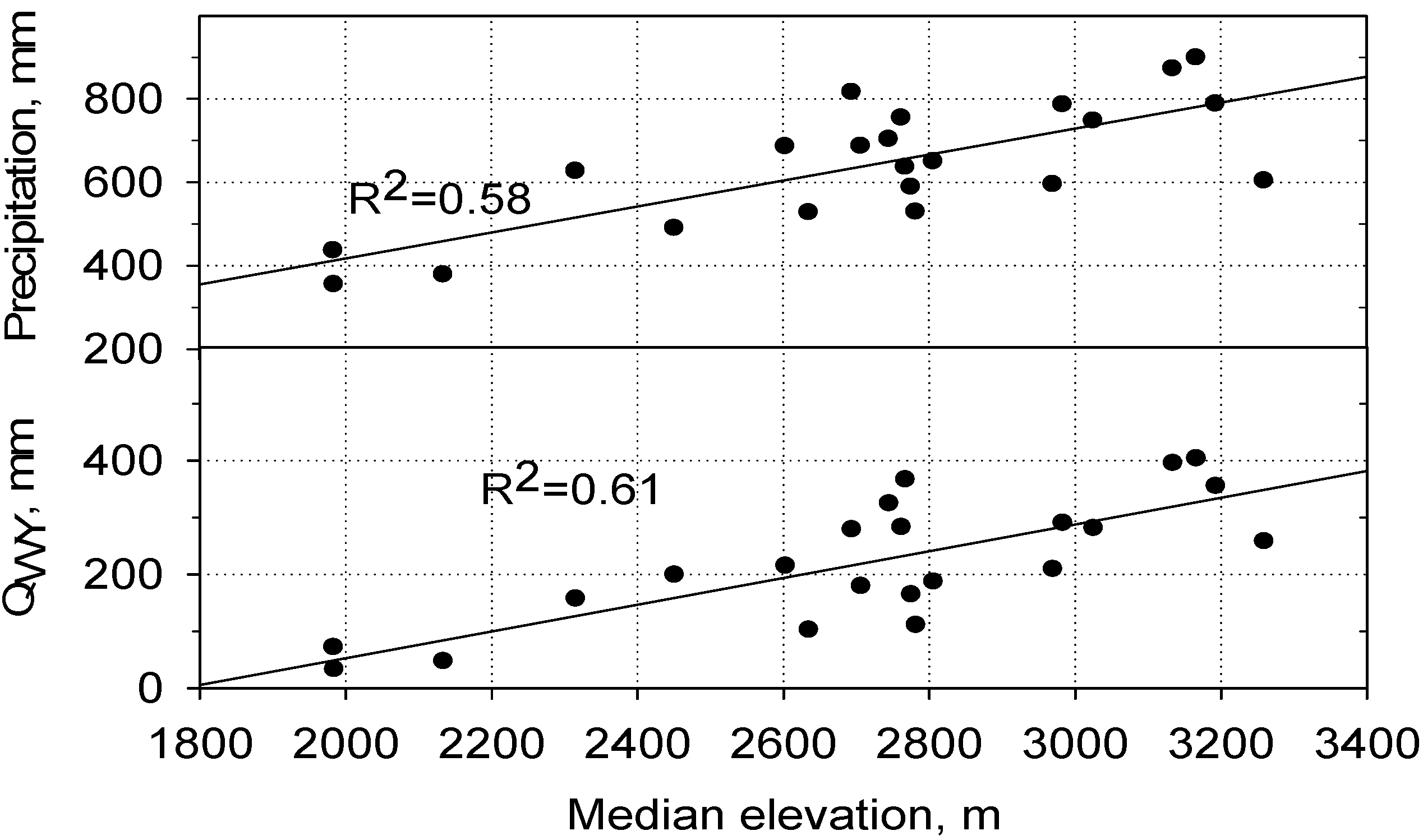
In Figure 3, the mean precipitation for the Colorado River basin locations ranges from about 400 mm per year to about 900 mm per year [14]. The precipitation data were from PRISM, which are spatial datasets incorporating a wide range of climatic observations. Monthly precipitation for the years of record were downloaded from PRISM and average precipitation was calculated for each basin. The interannual variability of water-year streamflow and precipitation is shown in Figure 4. It is apparent that runoff has a higher variability than does precipitation. In Figure 5a, the increasing runoff from the watershed follows the increasing water-year precipitation, with larger variability in the runoff. Figure 5b shows the precipitation along with the difference between precipitation and discharge, which is assumed to be mainly evapotranspiration. The evapotranspiration is fairly constant across the various locations, and is not correlated with elevation. In Figure 5c, the specific yield of water-year runoff is shown. Specific yield is the fraction of precipitation expressed as the water-year runoff. The specific yield has an increasing trend with increasing precipitation. The specific yield increases as mean watershed precipitation increases from less than 400 mm per year to approximately 700 mm per year (Figure 5a,c). The specific yield then appears to level off around 0.4 to 0.5. There is some variability especially with the observed flow (#17, #4, #15 and #28) vs. naturalized flow watersheds. In Figure 6a, the watershed precipitation is shown to be correlated with median watershed elevation. As the median elevation increases from 2000 to 2600 m, the water year precipitation increases from 400 to 600 mm. There is clustering in watersheds from 2600 to 2800 m, and at the highest watershed elevations of 3000 to 3300 m, where precipitation is near 800 mm. This clustering illustrates the variability in precipitation when compared to the median watershed elevations. In Figure 6b, the water year runoff is shown to be correlated with median elevation. This is a result of the fairly constant evapotranspiration amount.

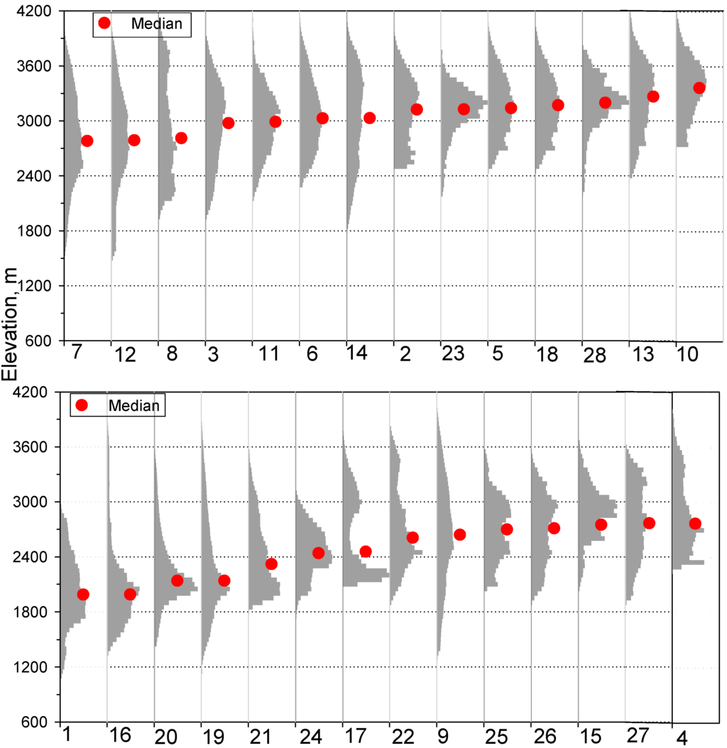
Figure 2. Elevation histogram and median elevation for the 28 watersheds, sorted by elevation. Forecast location on abscissa (Table 4), and elevation is in meters on ordinate.

Figure 2. Elevation histogram and median elevation for the 28 watersheds, sorted by elevation. Forecast location on abscissa (Table 4), and elevation is in meters on ordinate.

Figure 3. Mean water year precipitation for 28 Colorado River basin watersheds ± one standard deviation over the period of record for each location (PRISM data).

Figure 3. Mean water year precipitation for 28 Colorado River basin watersheds ± one standard deviation over the period of record for each location (PRISM data).

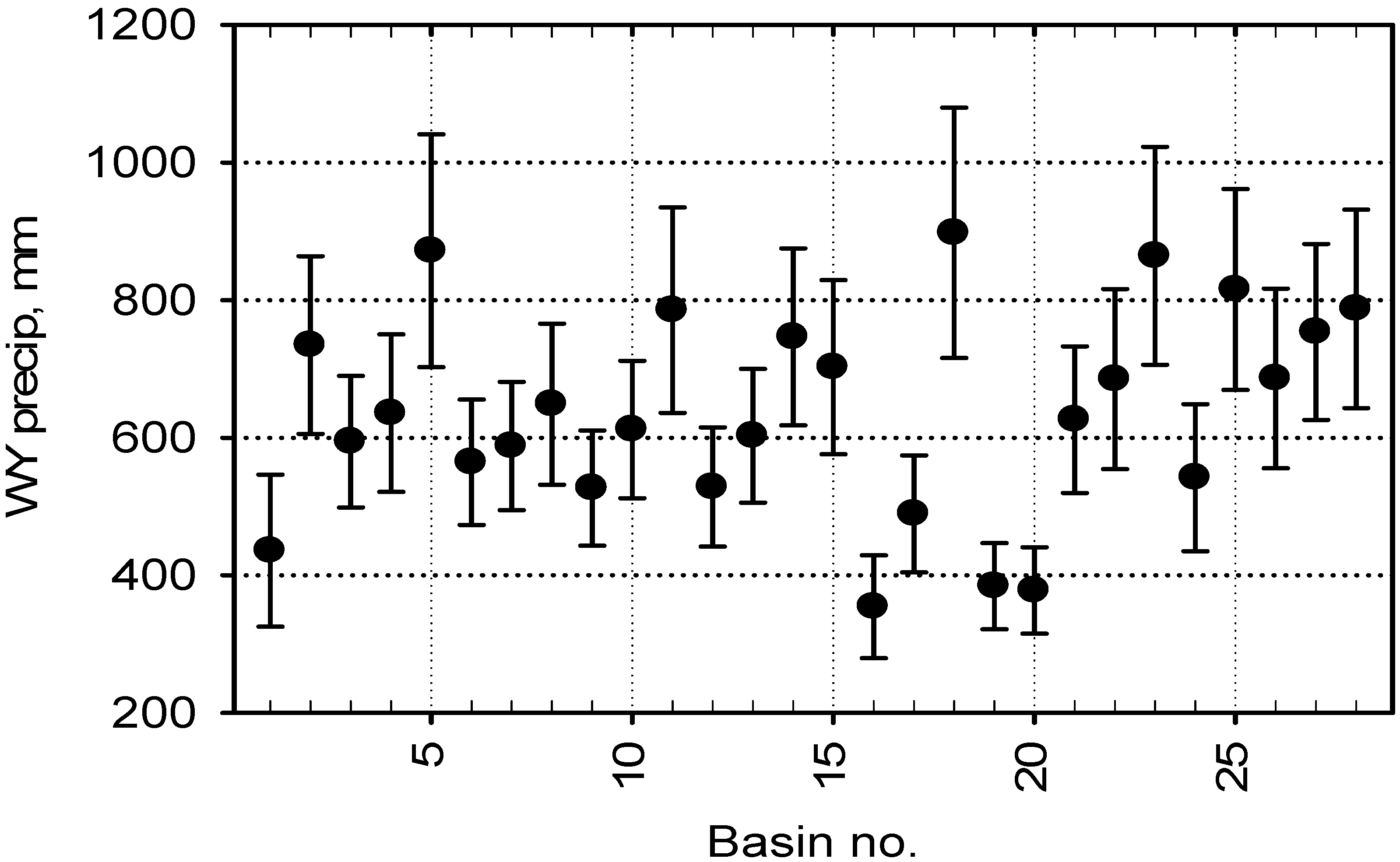
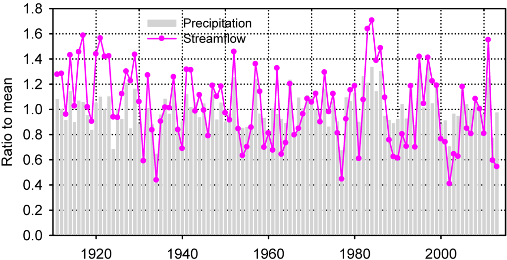
Figure 4. Ratio to mean water-year runoff and ratio to mean water year precipitation across all basins.

Figure 4. Ratio to mean water-year runoff and ratio to mean water year precipitation across all basins.

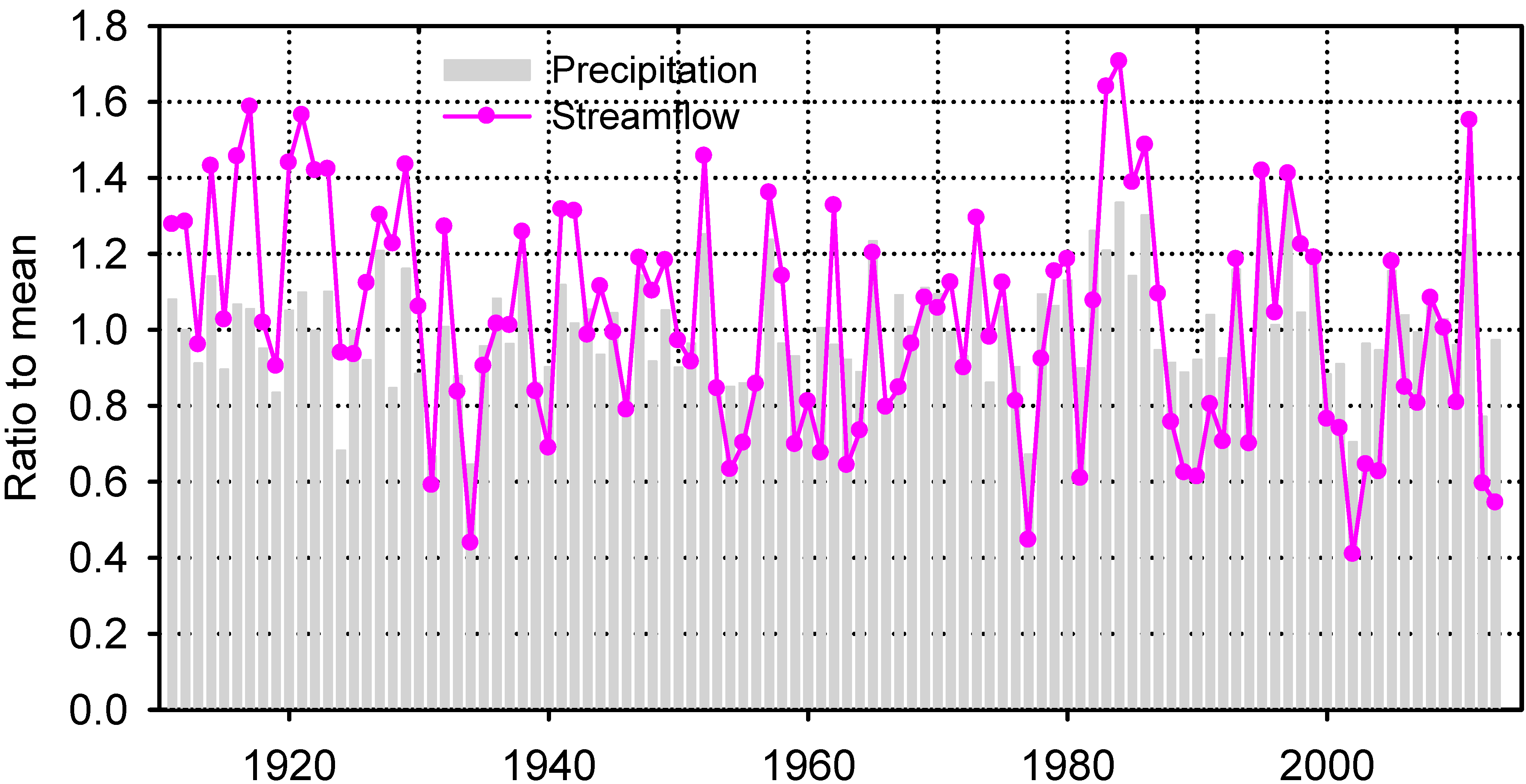
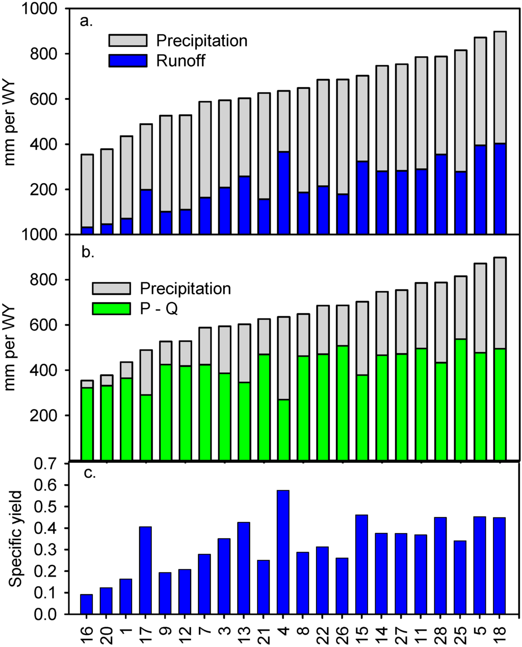
Figure 5. (a) Mean water year precipitation and runoff; (b) Mean water year precipitation and mean precipitation minus mean water year runoff; (c) Water year specific yield. All plotted by increasing precipitation with the basin indicated on the abscissa (Table 4). Six basins, not shown, had missing or inconsistent water-year data in the NWIS database (2, 6, 10, 19, 23, 24).

Figure 5. (a) Mean water year precipitation and runoff; (b) Mean water year precipitation and mean precipitation minus mean water year runoff; (c) Water year specific yield. All plotted by increasing precipitation with the basin indicated on the abscissa (Table 4). Six basins, not shown, had missing or inconsistent water-year data in the NWIS database (2, 6, 10, 19, 23, 24).

Figure 6. (a) Water year precipitation vs. watershed median elevation; (b) Water year runoff vs. watershed median elevation.

Figure 6. (a) Water year precipitation vs. watershed median elevation; (b) Water year runoff vs. watershed median elevation.

3. Results

3.1. Forecast Skill—Summary and Correlation Measures

The summary measure SSMAE was computed for each of the five forecast months, January to May, for each of the 28 forecast locations. Boxplots of the skill scores are shown in Figure 7. The forecast skill in January is quite low, with the SSMAE below 0.3 but with a tight distribution, as this early in the forecast season the forecasts may be made using average climatology. The forecasts in February contain additional winter-storm information and thus have higher skill but a wider distribution. The figure indicates that the runoff forecast skill increases from the start to end of the forecast period, with the Skill Score in March around 0.4, 0.5 in April, and ending the forecasts season in May with a Skill Score of approximately 0.6. The distribution widens more in March with no increase in skill. The width of the distribution in May remains wide when compared to the width of the forecast distribution in other months, in spite of the availability of additional information. There are several outliers for each month of the forecast season.

Figure 7. The skill scores for the Colorado River locations. (a) SSMAE. (b) NS score. The horizontal line within each box is the median of the 28 skill scores, with the box containing 25% to 75% of the scores. The two bars outside are 10% to 90% with the remaining points of the distribution shown as outliers.

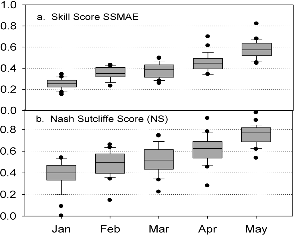
Figure 7. The skill scores for the Colorado River locations. (a) SSMAE. (b) NS score. The horizontal line within each box is the median of the 28 skill scores, with the box containing 25% to 75% of the scores. The two bars outside are 10% to 90% with the remaining points of the distribution shown as outliers.

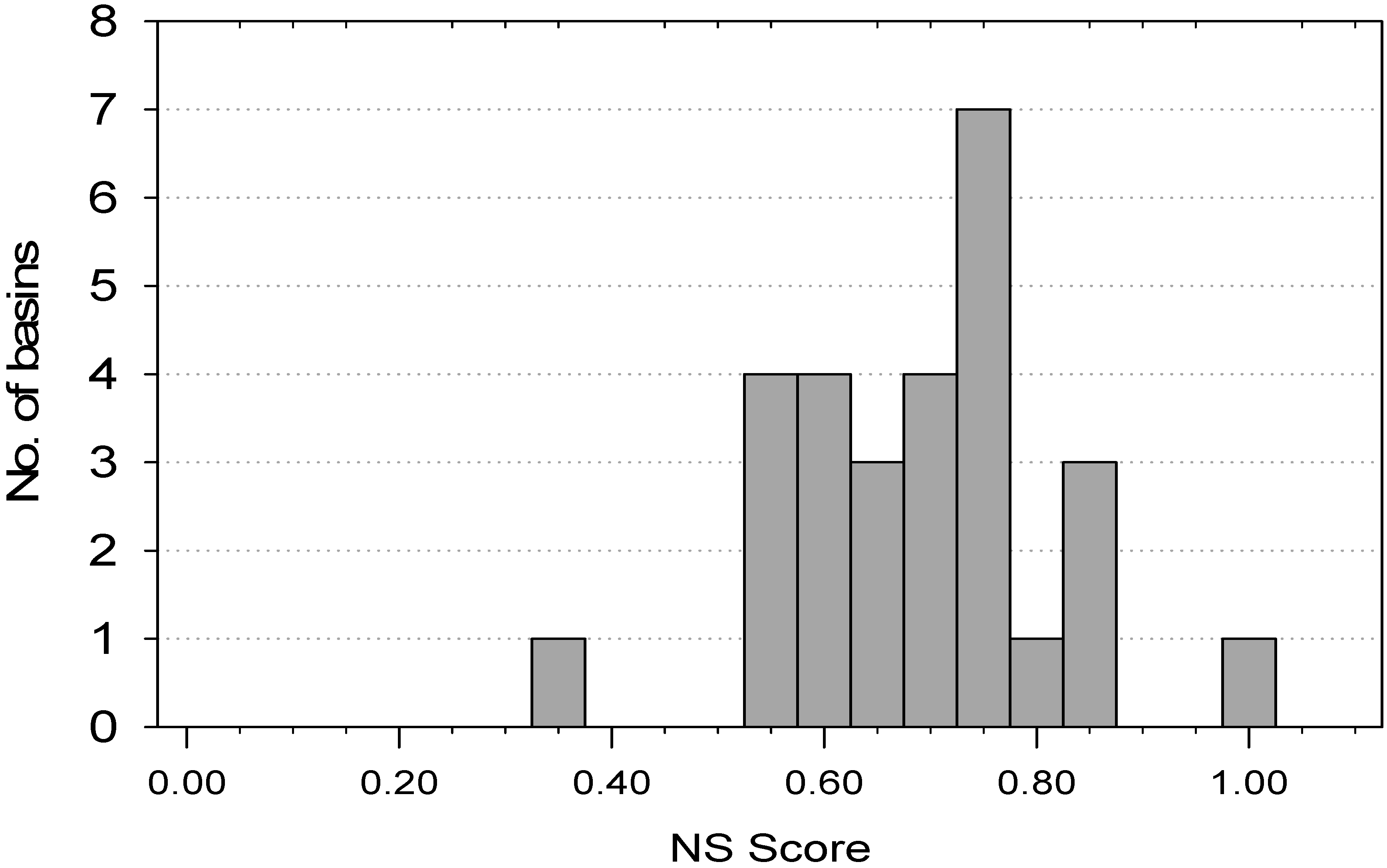
The correlation measure computed for the forecasts was the Nash-Sutcliff score. The distributions of NS for the five forecast months at the 28 forecast locations are shown in Figure 7b. The median January NS starts at 0.4 and steadily increases to 0.8 for the median in May. The width of the distribution increases remains steady through the forecast season with the increasing information available from March to May. The increase in skill as the forecast season progresses is clearly shown, but no change in distribution width is apparent. Outliers are present for all forecast months. In Figure 8, a histogram of the NS for April is shown. It suggests that the NS scores are distributed with a central tendency but not in a normal distribution.

Figure 8. NS score distribution for April.

Figure 8. NS score distribution for April.

3.2. Forecast Skill—Categorical Measures

The April–July runoff was categorized into low-runoff years (0 to 0.3), mid-runoff years (>0.3 to 0.7 and high-runoff years (>0.7), expressed as a fraction of the runoff occurrences for the period of record. The five categorical measures were calculated at each location for each of the three runoff categories. The first categorical measure is the Probability of Detection (POD) shown in Figure 9a. Mid runoff years show limited change in POD during the forecast season with the low and high-runoff years showing some improvement during the season. The median April POD for all three categories is above 0.7, but several sites still have values below 0.5.

The False Alarm Rate (FAR) shown in Figure 9b reinforces the difficulty of forecasting mid-flow years, as each year looks mid-flow early in the forecast season. Both the low- and mid-runoff years have a fairly high FAR early in the season, with the FAR dropping below 0.3 by the end of the season, but above 0.4 for mid flows in April. Interestingly, the high-flow FAR remains consistently low through the forecast season, potentially reflecting the lack of information and thus the reluctance of forecasting a “false alarm” for high-runoff years.

The Bias shown (Figure 9c) illustrates the effect of increasing knowledge through the forecast season. The Bias results show under forecast of both low- and high-flow years early in the forecast season, with a movement to little or no Bias by April. The Bias results show the over-forecast of mid runoff years early in the season as average climatology is assumed for the remainder of the forecast season. The mid flow forecasts also end the season with little or no bias. The Bias scores for the high runoff years show slight improvement through the forecast season, but remain under forecast even in April and May.

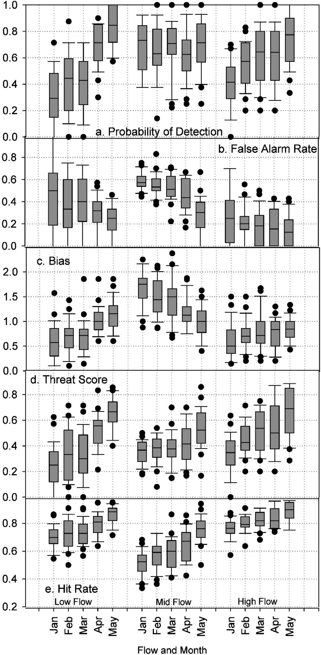
Figure 9. Categorical skill measures (a–e) for Colorado River basin. See Figure 7 for explanation of graphics.

Figure 9. Categorical skill measures (a–e) for Colorado River basin. See Figure 7 for explanation of graphics.

The Threat Score (TS) is shown in Figure 9d. The TS scores in January for low-runoff years start lower (0.25) than for mid (0.4) or high-runoff years (0.35). The TS also rises rapidly through the season, with the mid-runoff years remaining less skillful than the low or high-runoff years. This reflects the TS as solely a measure of correct forecasts.

The January Hit Rate (HR) (Figure 9e) starts higher in low-runoff years (0.7) and high-runoff years (0.75) than the January score for mid-flow years (0.55). The HR increases through the forecast season and for the April forecasts the HR is 0.8 for low and high flows, but for mid-flow years is approximately 0.65. The slightly lower scores for mid-flow years may reflect the occurrence of low or high flows for the season even if average flows occur during the early part of the forecast season. Note that HR values for low- and mid-flow years are higher than for the TS, reflecting its use as an index of both correct forecasts and non-forecasts.

4. Discussion

All measures during the forecast period show an increased in skill as more information becomes available on the amount of seasonal precipitation. The interpretation of this increase in skill is aided by recognizing that one of the measures, the SSMAE analysis, has the resolution necessary to pick up a widening distribution of forecast skill early in the forecast season through March. This trend may be related to the increase in difference between field conditions at the various forecast locations that cannot be described by the limited increase in knowledge of monitored conditions at the forecast points.

Another important interpretation of the previously found tight distribution of forecast skill levels is that unlike in the Sierra Nevada, no significant relationship was seen between watershed median elevation and increasing forecast skill, represented by April NS (Figure 10) or the categorical measures (not shown) [15]. This is because the Colorado River basin watersheds are similar in snow domination due to their sufficiently high elevation so that during major storms they experience precipitation mainly as snow. Unlike the Sierra Nevada, the Upper Colorado headwaters do not have a rain/snow transition. Thus it is variable precipitation amounts across this large basin, with storms from different origins and paths, rather than rain versus snow storms that affects skill.

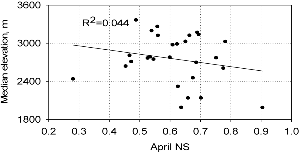
Figure 10. Relationship between April 1 NS and watershed median elevation.

Figure 10. Relationship between April 1 NS and watershed median elevation.

There is a strong correlation between the accumulation of the seasonal precipitation and the increase in skill in runoff forecasts. In order to interpret this relationship, SWE and precipitation data were obtained from the NRCS for 5 locations within the Colorado River basin and the average accumulations were calculated for each month in the water year (Figure 11) [16]. In February the average NS for the 28 locations is 0.48, with the cumulative snow at 0.75 and cumulative precipitation at 0.50 (Figure 7 and Figure 11). The NS and cumulative precipitation and snow increase in April to an NS of 0.61 with all of the snow and 0.73 of the yearly precipitation. In May, the NS increases to 0.75 with all of the snow and 0.80 of the yearly precipitation. As more of the seasonal precipitation falls, is measured and incorporated into the runoff forecasts, the skill of the forecast increases. The relationship is confirmed by the NS to snow correlation coefficient of 0.96 and a NS to precipitation correlation coefficient of 0.97.

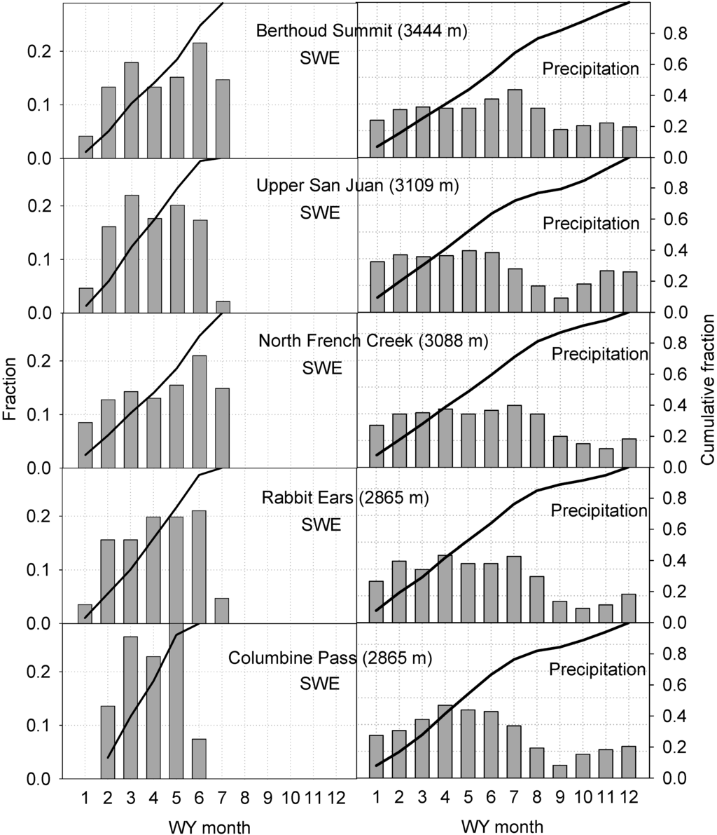
Figure 11. Monthly SWE and precipitation with accumulation. Data from NRCS, 1981–2010. Bars show monthly fraction, and lines the WY cumulative amount.

Figure 11. Monthly SWE and precipitation with accumulation. Data from NRCS, 1981–2010. Bars show monthly fraction, and lines the WY cumulative amount.

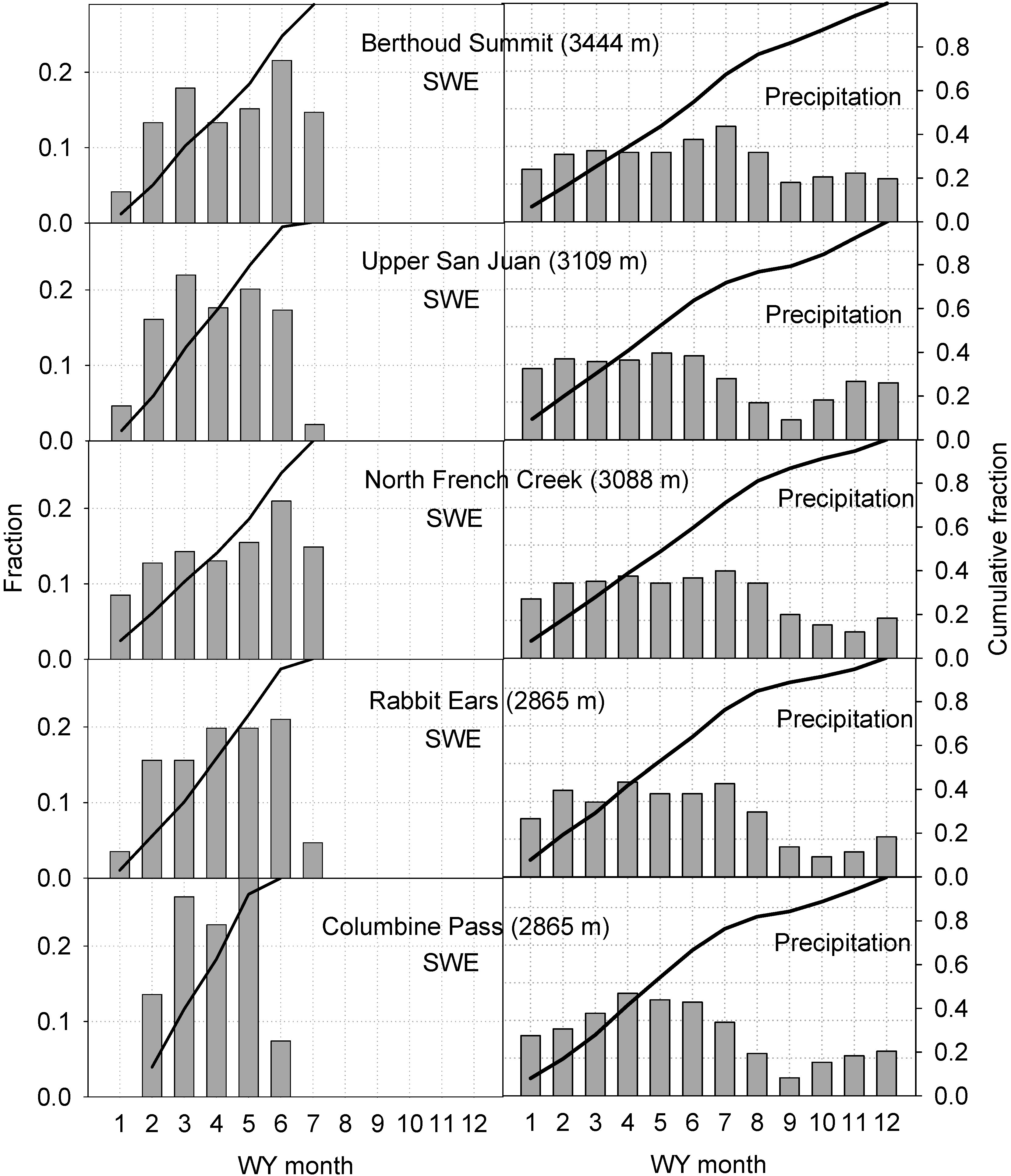
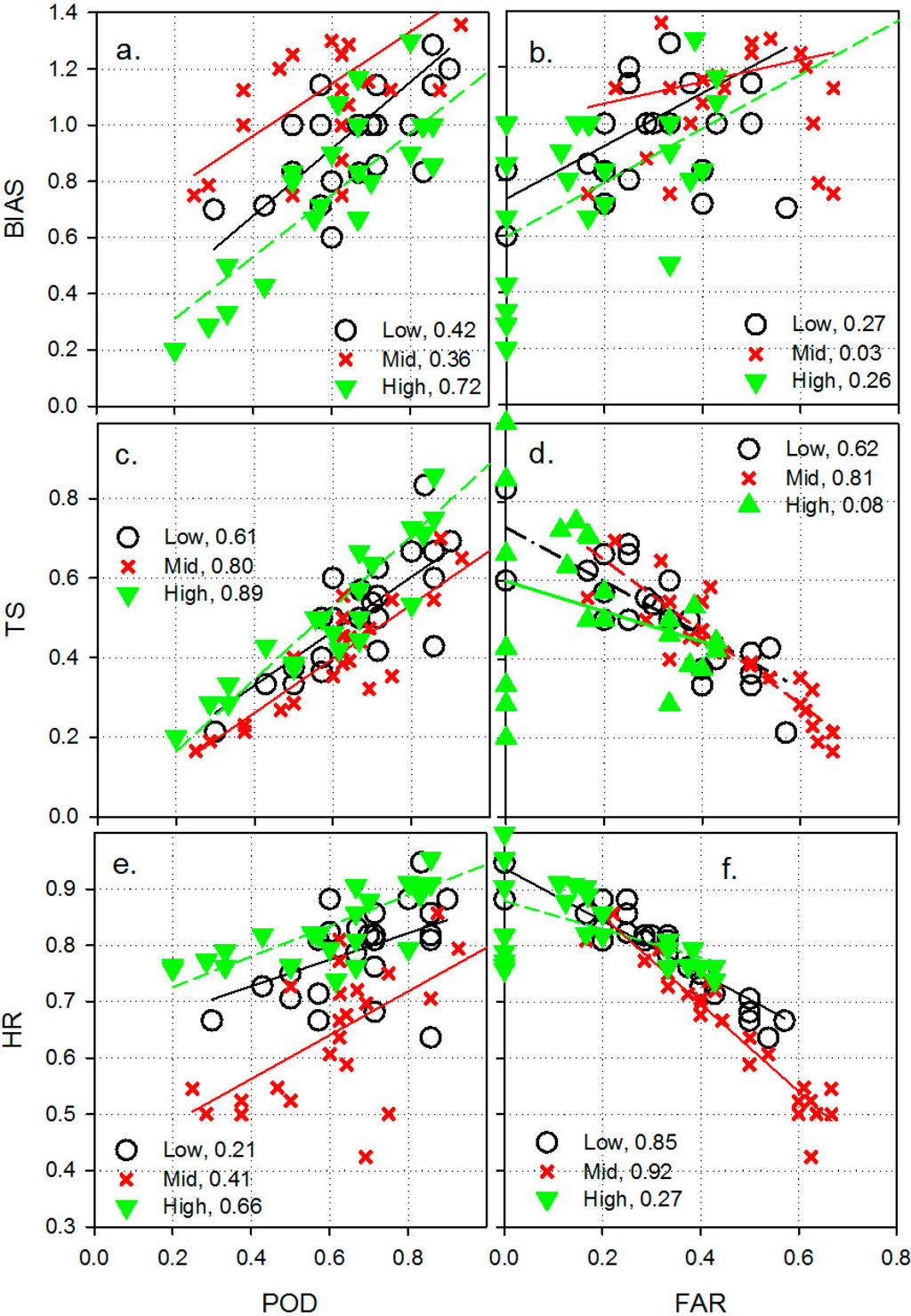
Figure 12. Correlation between categorical measures (a–f). Values in legend of each panel are R².

Figure 12. Correlation between categorical measures (a–f). Values in legend of each panel are R².

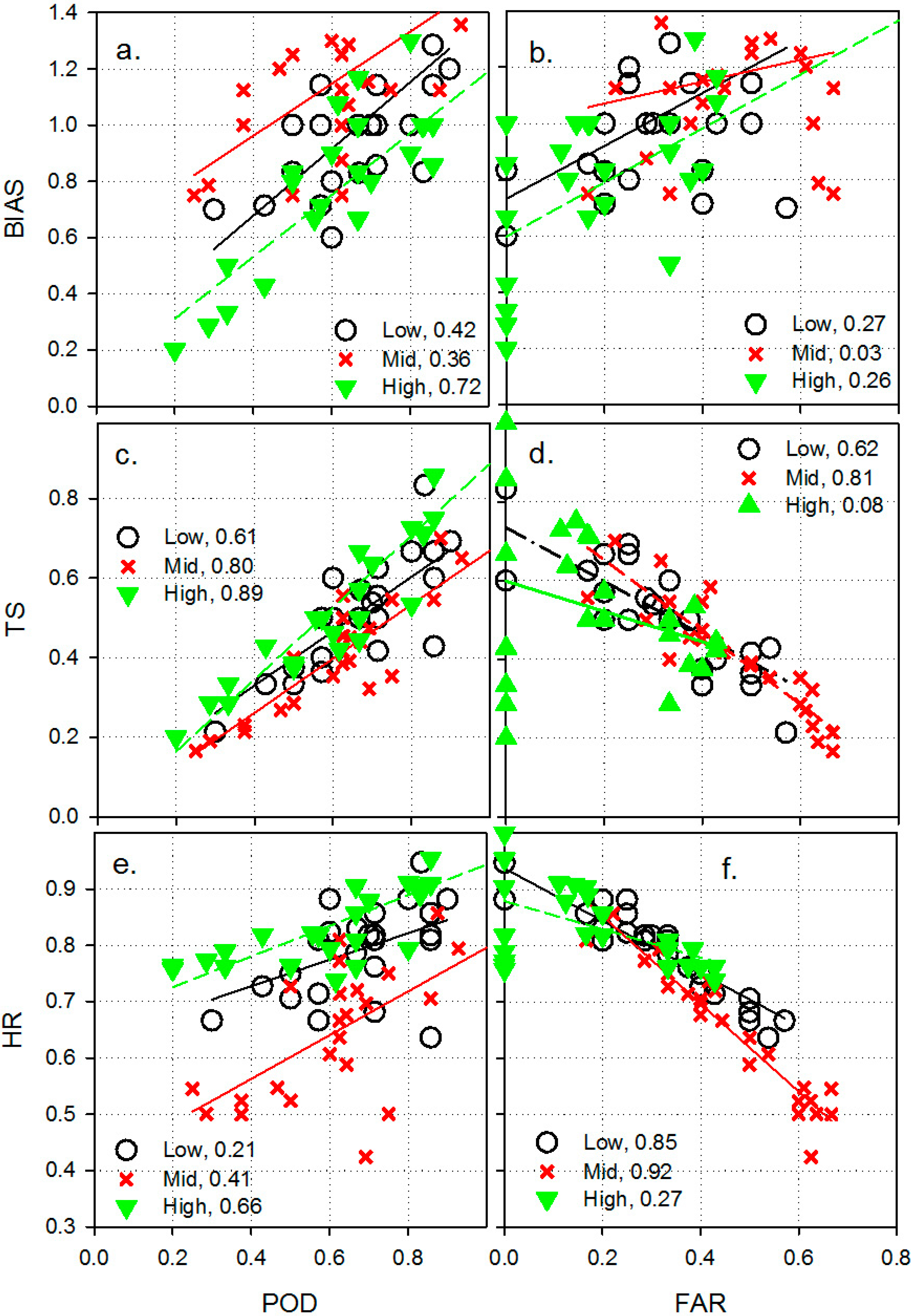
Of the categorical measures, POD and FAR are the simplest mathematically and conceptually straightforward. BIAS is correlated with POD for the high-flow category, suggesting that non-correct high-flow forecasts are not emphasized (Figure 12). Figure 12 is included to interpret the relationships between the various categorical measures and to enhance their usefulness by presenting correlations between the categorical measures. However, the lack of correlation between BIAS and POD for mid-flows reflects the high number of incorrect mid-flow forecasts for April. The lower importance of incorrect high-flow forecasts is also reflected in the similar correlation between TS and POD, as between BIAS and POD. Note that TS differs from POD by including incorrect forecasts in the denominator. The higher correlations between TS and POD for high and mid flows, versus the correlations for BIAS and POD, also reflect the addition of incorrect forecasts. But in the case of TS, the incorrect forecasts are in the denominator, resulting in lower TS versus POD values. Note that slopes of the TS and POD correlations are near 1.0 for all flows. This is also shown in the high correlation between TS and FAR for low and mid flows. HR differs from TS by including correct non-forecasts in both the numerator and denominator. The HR values vary less than POD values, illustrating the effect of correct non-forecasts. Note also a very high correlation between HR and FAR for all categories, because of the influence of correct non-forecasts.

It is useful to compare the forecast skill for the two types of flow conditions in the Colorado Basin, observed flow and naturalized flow. The forecast skill at the start of the forecast season in January is about 0.38 for both types of flows. The NS score increases for both flow conditions during February, March and April but the forecasts at naturalized flow locations are consistently lower in skill (April NS = 0.49) than the observed flow locations (April NS = 0.67). By the end of the forecast season in May, the gap has narrowed to 0.74 for naturalized and 0.78 for observed flow. Thus the starting and ending skill in the forecast seasons are approximately the same for the two very different flow types, but the mid-period forecasts (February to April) appear more skillful for the observed flow locations. This result probably reflects the complicating effects of diversions and storage on flow measurements during the late winter and early spring high runoff periods. Other factors that may affect runoff forecast skill include the percentage of water year precipitation that occurs in the January to March period, and the amount of base flow from the watershed in the winter.

While snowmelt accounts for much of the runoff across the basins evaluated, a shift from snow to rain under a warmer climate should reduce the ability of index measurements of snow to predict seasonal runoff. That is, the Colorado River basin may become more like the Sierra Nevada basins which currently have a mixed snowmelt and rainfall runoff [15]. In a warmer climate, some factors that affect forecast skill would include more variability of unknown future precipitation, effect of changes in sublimation on snowmelt, and increased river flow variability [17].

With climate warming, some water-supply forecasters may consider use of forecasting tools and data that are based on principles of mass balance and on the spatially distributed data needed to drive the models. Although current modeling tools are sufficiently flexible to incorporate immediate and larger future changes in climate that are outside the current stationarity assumption, data for those models are largely lacking. One other effect of changing climate is projected to be an increase in the amount of total precipitation falling as rain, emphasizing the potential of distributed, representative rainfall, as well as snowfall measurements to enhance forecasts. Future increases in skill level could be enabled by incorporating snow cover data estimated by remote sensing blended with representative ground measurements into the forecasting process. Increased forecast skill earlier in the water year, if new measurements can facilitate that, can provide significant economic benefits to water users, and introduce flexibility and resiliency into water-management decisions.

5. Conclusions

The summary and correlation skill measures such as SSMAE and NS show that forecast skill improves during the seasonal forecast period. They can also assess skill over multi-year periods; but getting year-by-year skill values would require use of an index such as percent bias (PBias). PBias would generate a time series of a skill index at a specific forecast location that can be reviewed for changes in forecast skill over time. Current analysis of PBias for the 28 locations in the Colorado River basin shows no indication of a long-term trend in forecast skill at those locations [18].

The use of multiple measures increases confidence that the chosen skill measures may have the resolution necessary to capture subtle changes, such as the increase in forecast uncertainty early in the forecast season. The categorical skill measures can appraise forecast skill for three different flow scenarios and show changes over the forecast period. For example, the FAR clearly shows a tendency to under forecast high flows, and the Bias shows the tendency to over forecast mid flows early in the season. Together, POD, FAR and Bias can be a good diagnostic for the region.

Examination of the hydrologic characteristics of the basins in the study indicated an increase in precipitation and runoff with increasing basin elevation. However, no relationship between forecast skill, as measured by the NS score, and watershed median elevation was found. This indicated that the watersheds in the Colorado basin have similar snow dominance of runoff. Variability in watershed orientation or precipitation is therefore more important in predicting forecast skill.

NS and MAE scores for the Colorado basin are generally lower than for the Sierra Nevada, which can introduce greater uncertainty into reservoir operations and water allocations. This may be offset in part by the greater relative amount of storage in Colorado River vs. Sierra Nevada reservoirs. Categorical measures also reflect less skill in the Colorado vs. Sierra Nevada [15].

References

- Pagano, T.; Garen, D.; Sorooshian, S. Evaluation of official western US seasonal water supply outlooks, 1922–2002. J. Hydrometeorol. 2004, 5, 896–909. [Google Scholar] [CrossRef]
- Bender, S.; Colorado Basin River Forecast Center, Salt Lake City, UT, USA. Personal communication, 2013.
- Work, R.A.; Beaumont, R.T. Basic data characteristics in relation to runoff forecast accuracy. In Proceedings of Western Snow Conference, Bozeman, MT, USA, 16–18 April 1958; pp. 45–53.
- Kohler, M.A. Preliminary report on evaluating the utility of water supply forecasts. In Proceedings of Western Snow Conference, Reno, NV, USA, 21–23 April 1959; pp. 26–33.
- Shafer, B.A.; Huddleston, J.M. Analysis of seasonal volume streamflow forecast errors in the western United States. In Proceedings of A Critical Assessment of Forecasting in Water Quality Goals in Western Water Resource Management, Bethesda, MD, USA, 11–13 June 1984; pp. 117–126.
- Schaake, J.C.; Peck, E.L. Analysis of water supply forecasts. In Proceedings of Western Snow Conference, Boulder, CO, USA, 16–18 April 1985; pp. 44–53.
- Dracup, J.A.; Haynes, D.L.; Abramson, S.D. Accuracy of hydrologic forecasts. In Proceedings of Western Snow Conference, Boulder, CO, USA, 16–18 April 1985; pp. 13–24.
- Hartmann, H.C.; Bales, R.; Sorooshian, S. Weather, climate, and hydrologic forecasting for the US southwest: A survey. Clim. Res. 2002, 21, 239–258. [Google Scholar] [CrossRef]
- Franz, K.J.; Hartmann, H.C.; Sorooshian, S.; Bales, R. Verification of national weather service ensemble streamflow predictions for water supply forecasting in the colorado river basin. J. Hydrometeorol. 2003, 4, 1105–1118. [Google Scholar] [CrossRef]
- Hartmann, H.C.; Morrill, J.C.; Bales, R. A Baseline for Identifying Improvements in Hydrologic Forecasts: Assessment of Water Supply Outlooks for the Colorado River Basin. In Proceedings of AGU Fall Meeting, San Francisco, CA, USA, 11–15 December 2006. Abstract H53C-0649.
- Morrill, J.C.; Hartmann, H.C.; Bales, R.C. An Assessment of Seasonal Water Supply Outlooks in the Colorado River Basin; Working Paper; Dept. of Hydrology and Water Resources, University of Arizona: Tucson, AZ, USA, 2007. [Google Scholar]
- Wilks, D.S. Statistical Methods in the Atmospheric Sciences; Elsevier: Oxford, UK, 2011. [Google Scholar]
- USGS National Water Information System. Available online: http://waterdata.usgs.gov/nwis (accessed on 3 March 2014).
- PRISM, PRISM Climate Group, Oregon State University. Available online: http://prism.oregonstate.edu (accessed on 15 September 2014).
- Harrison, B.; Bales, R. Skill assessment of water supply forecasts for western Sierra Nevada watersheds. J. Hydrol. Eng. 2015. submitted. [Google Scholar]
- NRCS Snotel Data. Available online: www.wcc.nrcs.usda.gov/snow (accessed on 11 December 2014).
- Decision-Support Experiments and Evaluations using Seasonal-to-Interannual Forecasts and Observational Data: A Focus on Water Resources. Available online: http://downloads.globalchange.gov/sap/sap5-3/sap5-3-final-all.pdf (accessed on 8 July 2015).
- Harrison, B.; Bales, R. Percent bias assessment of water supply outlooks in the Colorado River basin. In Proceedings of 82nd Annual Western Snow Conference, Durango, CO, USA, 14–17 April 2014; pp. 91–100.
© 2015 by the authors; licensee MDPI, Basel, Switzerland. This article is an open access article distributed under the terms and conditions of the Creative Commons Attribution license (http://creativecommons.org/licenses/by/4.0/).