1. Introduction
The Upper Blue Nile basin is one of the basins which has been affected by climate change, as well as catchment characteristics alteration due to the natural or anthropogenic activities, which may lead to extreme events such as drought and flood [
1,
2]. These chronic factors modify the normal functioning of the hydrologic cycle of the basin, which in turn alters the hydrological processes in the basin [
3]. Thus, for successful management and planning of water resources, a thorough understanding of the hydrological processes of the basin is crucial.
Hydrological models have been widely applied for comprehending these processes over the past few decades [
4,
5]. The models represent the catchment processes in a simplified way. They can be categorized as distributed and lumped models based on the way they represent the hydrological processes in the catchment [
6].
The distributed hydrological models characterize the catchment in details, but intensive data are required which are not available in most developing countries [
7]. However, if the catchment data (i.e., topography, soil and land use maps) are available in addition to precipitation and evapotranspiration information, they have a high importance in reproducing the runoff for the catchments with no streamflow record to assist water infrastructure investments [
8,
9,
10]. Distributed hydrological models represent the heterogeneity of the catchment by considering the spatial variability of hydrometeorological variables, topography, geology, soil type and land use. Nevertheless, their complexity, long computation time and enormous data requirement lead them to have a limited practicality in most contexts [
11]. Typical examples include the System Hydrologique European (SHE) model [
12] and Institute of Hydrology Distributed Model (IHDM) [
13].
On the other hand, lumped hydrological models represent the catchment as a single unit. They are characterized by minimal data requirement which is averaged over the catchment. In these types of models, the parameter values are determined through calibration, not from the physical behaviors of the catchment [
9]. In addition, the spatial inhomogeneities of the input variables and parameters are not represented, which limit their capability to simulate all of the hydrological processes of the catchment. Thus, only the dominant ones are properly described. Examples of these models include the Hydrologiska Byrans Vattenavdelning (HBV) [
14], Sacramento soil moisture accounting model [
15] and physically-based runoff production model (TOPMODEL) [
16]. For the study catchment, only hydrometeorological data are available. Thus, preference was given to lumped hydrological models as they only require hydrometeorological data as input for hydrological simulation.
The understanding of hydrological processes at catchment scale is very limited in the Upper Blue Nile basin. Most of the hydrological investigations have been focused on the basin scale with the outlet at ElDiem near the Ethio-Sudanese border and the head water of the basin, particularly the Tana basin [
17]. In addition, most of the studies conducted were based on a single conceptual hydrological model. Relying on single lumped hydrological model may lead to incorrect decisions for water resource management and planning, particularly in a data scarce basin such as the Upper Blue Nile basin, due to uncertainty in the model [
18,
19]. Thus, studies based on the use of multiple models may give a more concrete basis for decision making.
Moreover, only limited studies have been reported in the literature on quantifying the hydrological processes of the catchments in the southern and southwestern parts of the Upper Blue Nile basin [
17,
20,
21]. Thus, this study is conducted with objectives to (1) predict the stream flow of the Upper Guder catchment in southwestern of the Upper Blue Nile basin; and (2) to intercompare the performances of the models in predicting the flow.
2. Materials and Methods
2.1. Study Catchment
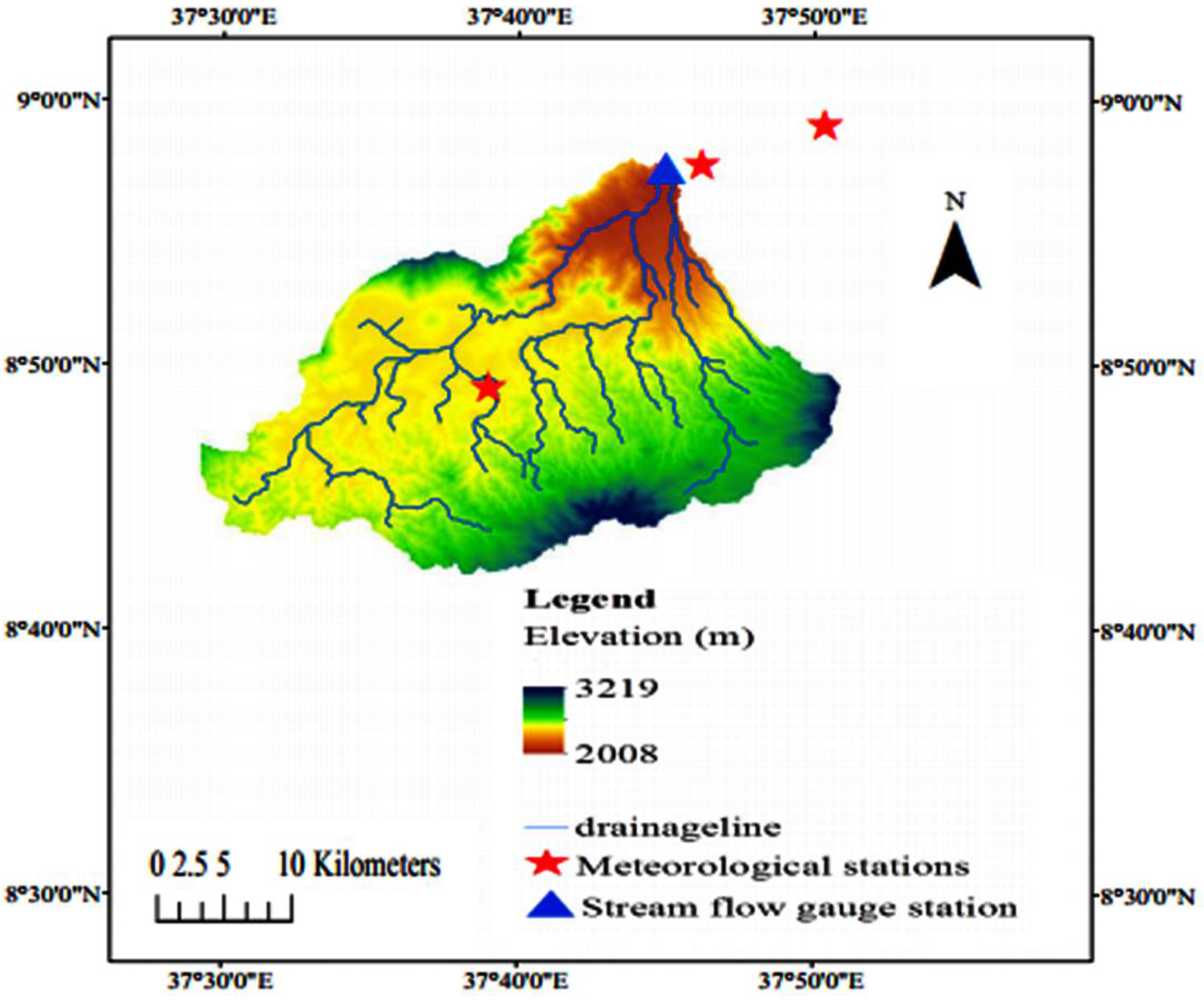
The upper Guder catchment is a sub-basin of the Guder basin in the upper Blue Nile basin which has an area of about 524 km
2 and is located within latitude 8°45′ and 9°22′ N and longitude 37°30′ and 37°70′ E (
Figure 1). The catchment was delineated from the Digital Elevation Model (DEM) obtained from the Shuttle Radar Topographic Mission (SRTM) acquired from the Consortium for Spatial Information (CGIR-CSI) website (
http://srtm.csi.cgiar.org/, last accessed on 4 June 2017). The Guder River starts from the mountainous area of South of Ambo and Guder towns at an elevation of 3000 m above sea level. It collects water from a number of streams (i.e., Huluka, Fatto, Indris and Debis) along its way to the lower Guder, where it meets the Blue Nile river. The catchment obtains most of its rainfall from June to September. The main economic activity in this catchment is rainfed-agriculture. Soils that are predominantly available in the catchment include Vetisols, Latosols, Cambisols, Alisols, Luvisols and Nitisols [
22].
2.2. Hydro-Meteorological Data
The daily rainfall and temperature data from the stations within and nearby the catchment were used as the inputs to the models. There is only one station (Tikur Inchini) within the catchment, whereas Guder and Ambo are the stations located close to the catchment. The daily potential evapotranspiration (PET) was calculated by making use of the Hargreaves method. This method requires maximum and minimum temperature to estimate potential evapotransipration and it is widely used in data scarce regions due to its minimal data requirement [
23].
The meteorological and flow data were obtained from National Meteorological Service Agency (NMSA) and the Ministry of Water, Irrigation and Energy in Ethiopia (MOWIE), respectively (
Table 1).
2.3. Lumped Conceptual Rainfall-Runoff Models
Lumped conceptual rainfall-runoff models have been widely applied, particularly in data scarce regions. They describe the most important hydrological processes by a set of solvable mathematical equations. The inputs to the models are averaged over the catchment while representing it as a single unit [
18,
24]. The general structure of most of the lumped models is similar. Soil moisture storage and subflows are the main components of the models. In addition, the lumped models comprise the routing module, which is typically the linear reservoir model [
25]. The Veralgemeend Conceptueel Hydrologisch (VHM) and Nedborafstromnings model (NAM) models were employed for this study. They have a similar model structure and need hydrometeorological data to predict the discharge [
24].
2.4. VHM Model
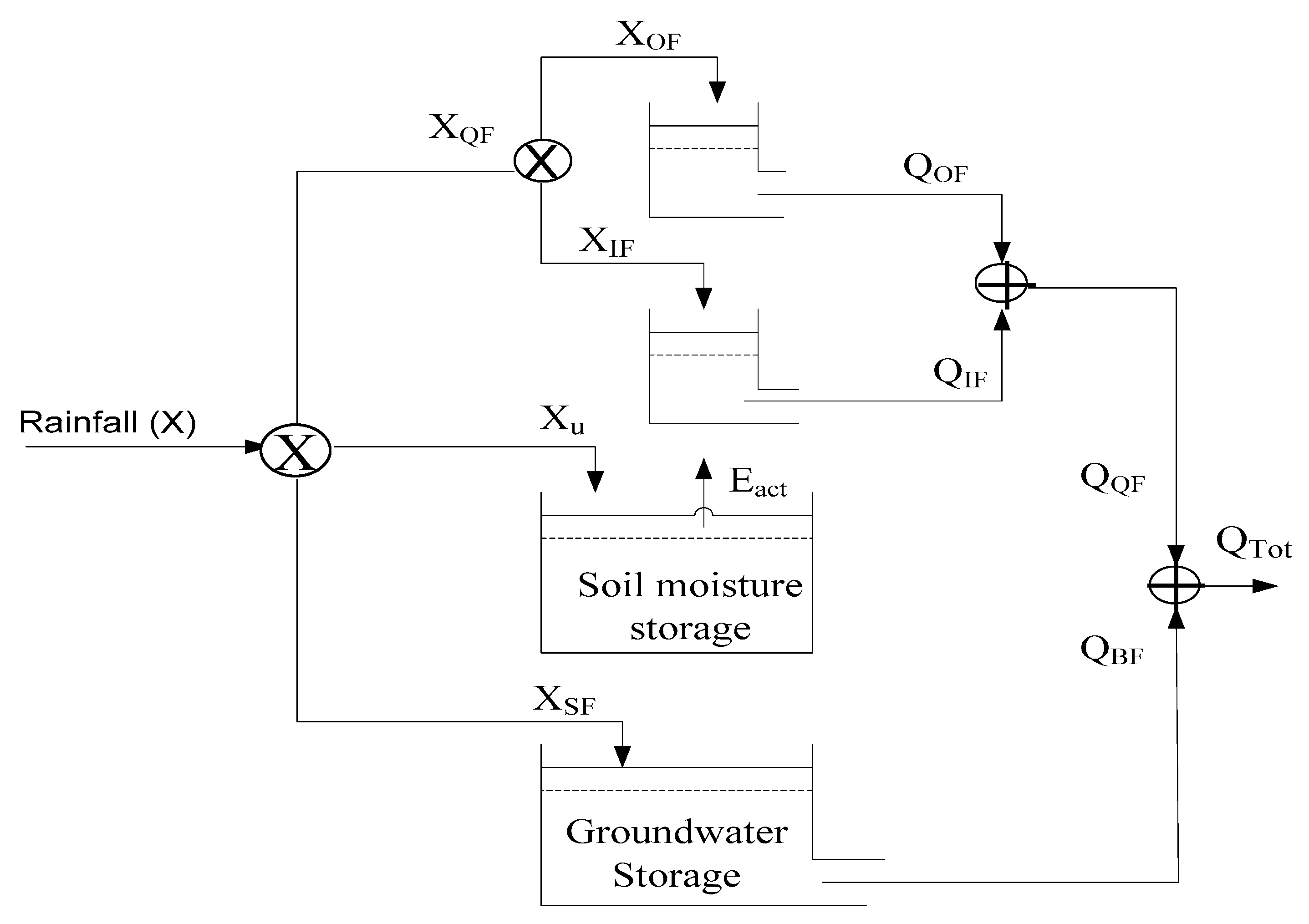
The VHM is a lumped conceptual rainfall–runoff model which represents the Dutch abbreviation of “Veralgemeend Conceptueel Hydrologisch” and refers to “generalized lumped conceptual and parsimonious model structure identification and calibration”. It consists of soil moisture storage, interflow, overland flow and routing sub-models. Areal rainfall and potential evapotranspiration were estimated using the Thiessen polygon interpolation method and were used as the inputs to the model. The subflow components and total discharge were provided as additional inputs to the model. The rainfall input to the model was shared between the soil moisture storage and the sub-flow components (
Figure 2). This needs to be modeled to know the amount contributed to soil moisture storage and the subflow components. The amount of rainfall contributed to the subflows is routed and added to give the total flow [
25,
26]. The calibration parameters and variables of the VHM model are given in
Table 2.
2.5. NAM Model
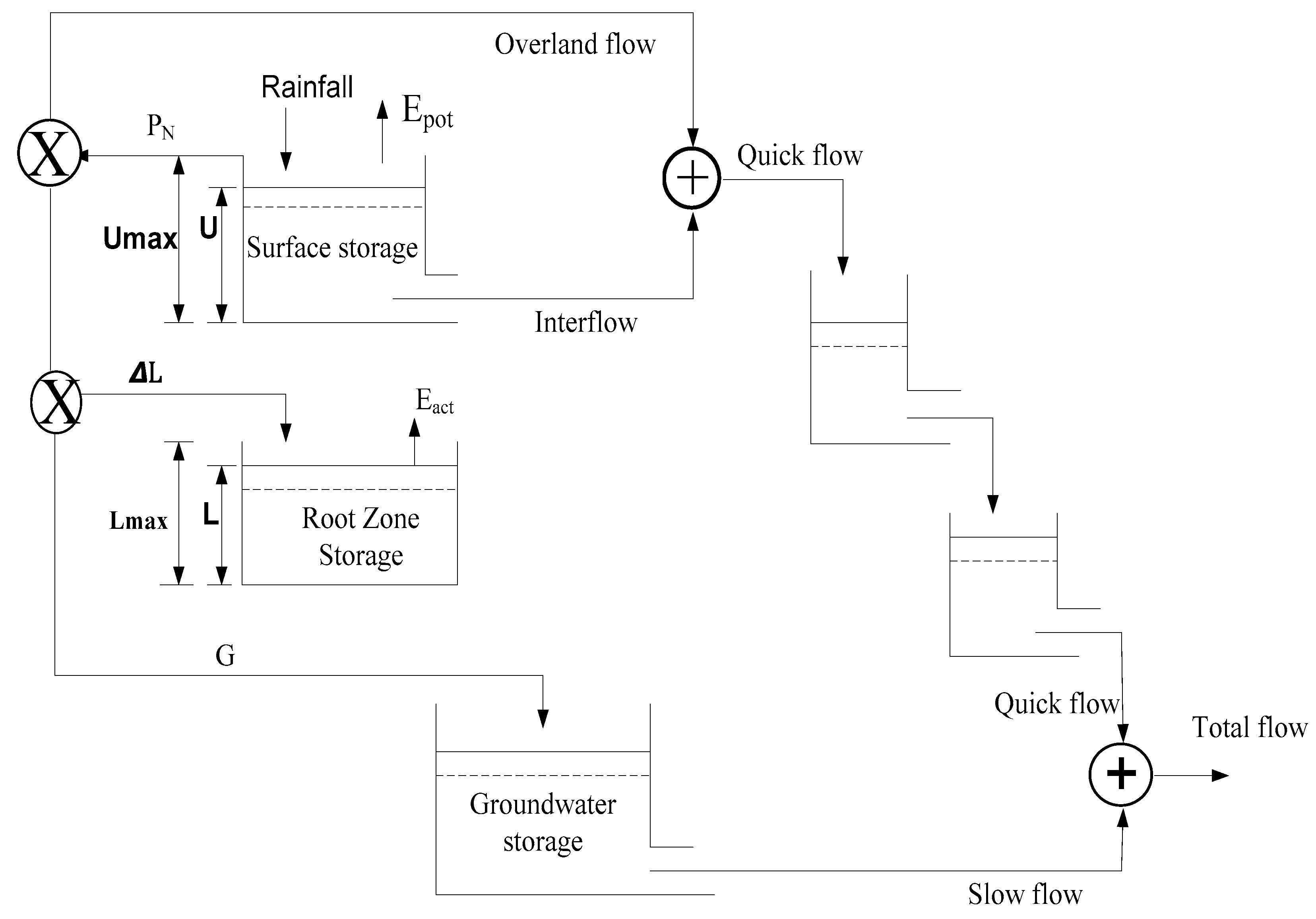
The NAM is a Danish abbreviation which stands for NedborAfstromnings Model, meaning a rainfall–runoff model. It is developed at Technical University of Denmark, Department of Hydrodynamics and Water Resources. Similar to the VHM, catchment averaged rainfall and potential evapotransipration were used as the inputs to the model. The model consists of four interrelated storages to describe the hydrological cycle of the land phase (
Figure 3). These are snow, surface, lower zone and groundwater storage [
27,
28]. The snow storage is excluded in this study as there is no snow in the study catchment.
Surface storage represents the fraction of precipitation intercepted by plant canopy and ensnared in depression on the surface of the land. The water in this storage may be lost by evaporation and leakage to the stream in the form of interflow. On the other hand, if the storage is filled fully, the excess water may join the stream as the overland flow, whereas the remaining one is diverted in the form of infiltration and recharge to lower zone and ground water storage, respectively.
Lower zone storage represents the moisture stored within the root zone of the soil. Transpiration is responsible for the loss of water in this storage. The moisture content of the lower zone storage governs the amount of water that goes into overland flow, interflow and groundwater flow. Groundwater storage is responsible for the baseflow component [
28]. The calibration parameters and variables of the NAM model are given in
Table 3.
2.6. Intercomparision of the Models
The application of multiple models is important in reducing the uncertainty of the results of hydrological simulation and booming the confidence of decision making in water resources planning and management. The VHM and NAM models were applied to similar input data set and produced the streamflow as the output. The performances of the models are measured by same performances evaluation tools. The simulation results of the models were then compared.
2.7. Pre-Processing of Stream Flow Data
The Water Engineering Time Series PROcessing tool (WETSPRO) was employed to split the total flow into subflow components (i.e., overland flow, interflow and baseflow). The subflows are provided as inputs to the VHM model for calibration of the modeled subflow components.
The Chapman recursive digital filter was originally used to divide the streamflow into quick flow and base flow based on the recession constant (K) only [
29]. However, further modification was made through introduction of additional parameter called w-factor [
30]. The combination of the recession constant and w-factor split the total flow into its subflow components using the WETSPRO tool. The w-factor represents the average fraction of the sub-flow volume to the total flow volume, whereas the recession constant represents the time at which the flow gets reduced to 37% of its original flow during the dry season flow. In other words, it represents the time it takes for the catchment to respond to each sub-flow component. Its value was estimated as the inverse slope of the sub-flow recession periods of a
ln (
q)—time graph [
30]. The values of the recession constants estimated for each subflow component was used as the input to the models for initial model set up and subjected to slight adjustments to control the shape of the hydrograph (
Table 4).
2.8. Model Calibration
The models were manually calibrated with the objective to maximize the Nash Sutcliffe efficiency and minimize the water balance discrepancy, while considering a good overall agreement of the shape of the hydrograph of the observed and simulated flow. The period from 1 January 1990 to 31 December 2000 and from 1 January 2001 to 31 December 2005 were used for the model calibration and validation, respectively.
The VHM model calibration was based on the stepwise approach in which each module in the model is calibrated in a sequential way. It starts from the soil moisture storage module by tuning of the model parameters through trial and error. This procedure based approach increase the efficiency and transparency of the model [
25].
Even though the NAM model has an automatic calibration alternative, the manual calibration was favored to make both models comparable. The calibration of the NAM model was based on the different rainfall-runoff processes descriptions of the relevant model parameters [
28]. For instance, the water balance is controlled by Umax and Lmax, the distribution of excess rainfall between overland flow and infiltration is managed through tuning of CQOF, whereas the recession constant parameters (i.e., CKBF, CK
IF, and CK
1,2) control the shape of the hydrograph.
2.9. Model Performance Evaluation
Statistical and graphical means were used to evaluate the performances of the models. The widely used statistical method, Nash Sutcliffe Efficiency [
31], was calculated using Equation (1).
where NSE is the Nash Sutcliffe efficiency,
is simulated flow,
is observed flow,
is the average of the observed flow,
is the average of the simulated flow and
n represents the length of series.
In addition, the coefficient of determination (R
2) and water balance discrepancy (WBD) between the observed and simulated flow were calculated using Equations (2) and (3), respectively.
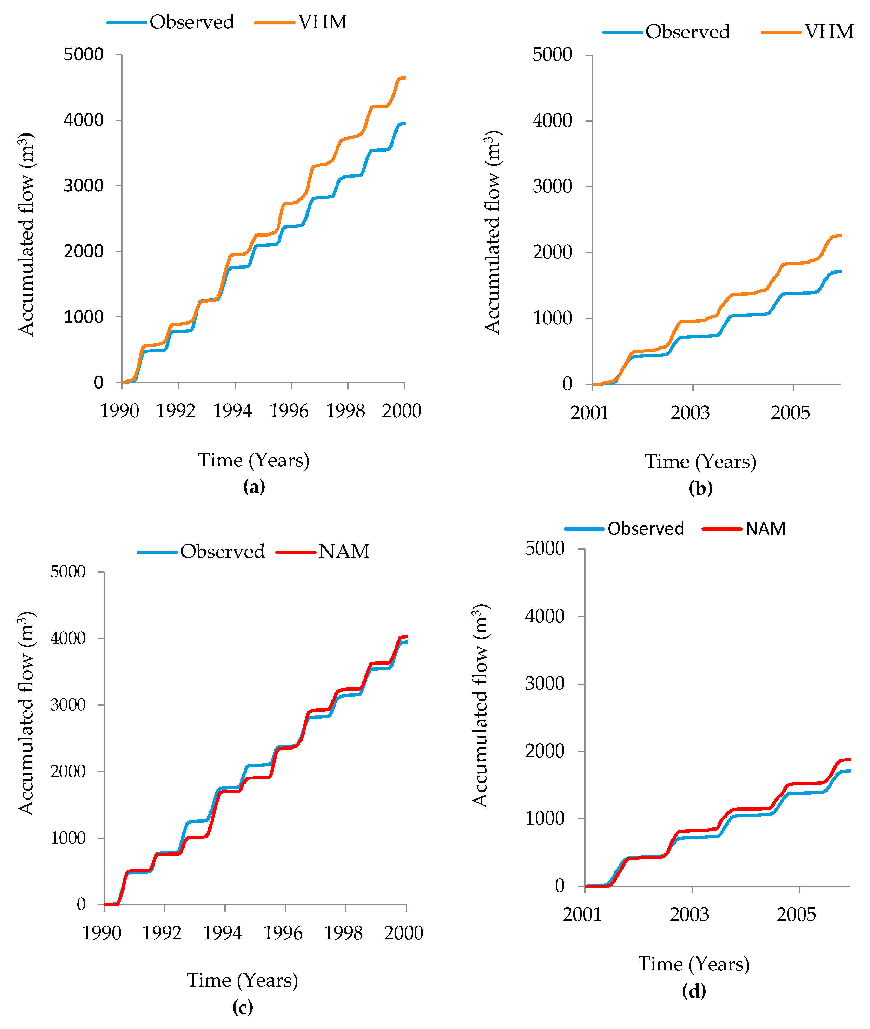
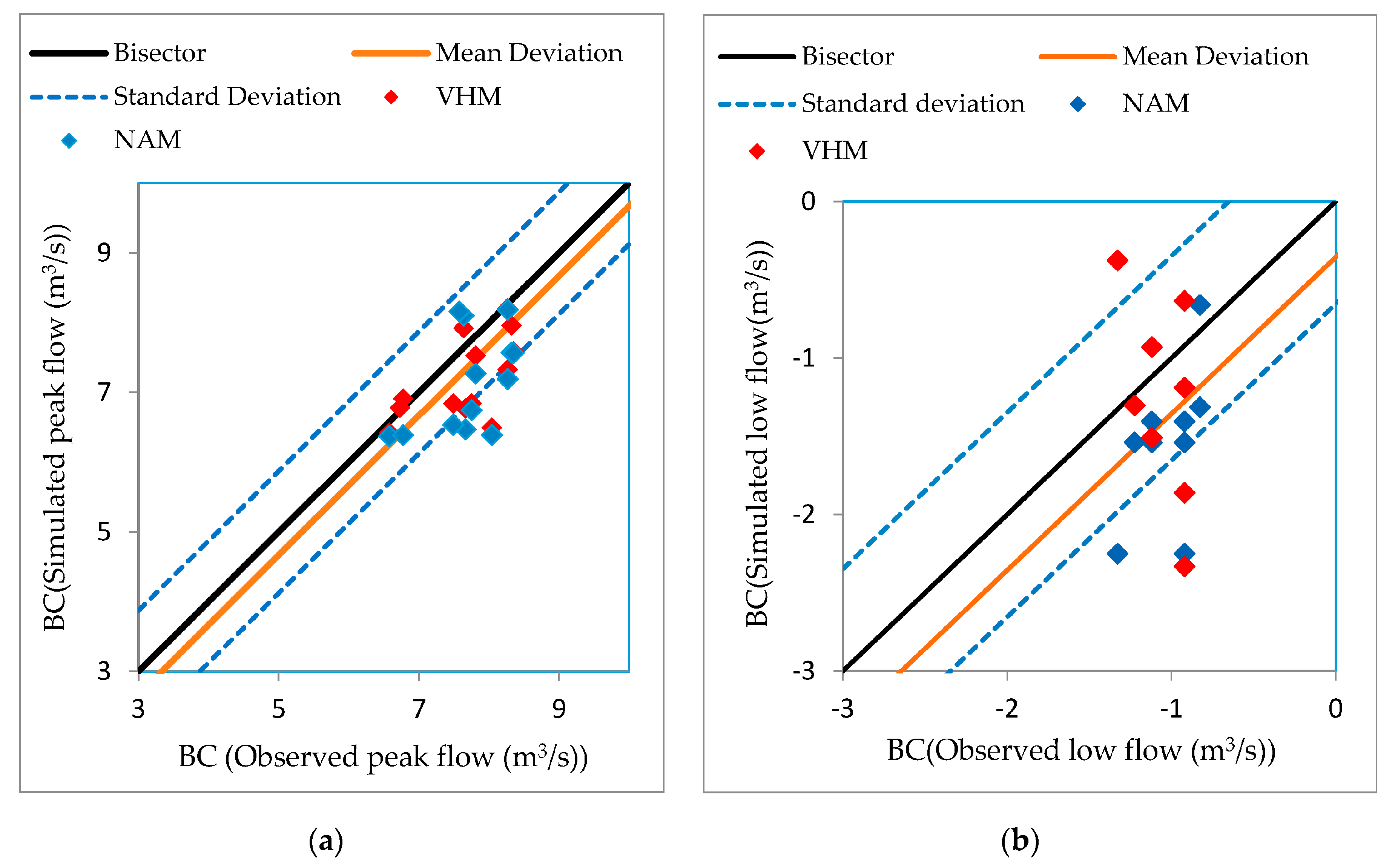
On the other hand, for visual comparisons graphical fitting and cumulative water balance between the observed and simulated flow were used. In addition, the performances of the models in simulating the peak and low flows were evaluated after the Box-Cox transformation [
32]. The nearly independent peak and low flows were selected using the WETSPRO tool and then a Box-Cox transformation was applied to them by using Equation (4).
where
Q is the peak flow and
is the Box-Cox transformation parameter. A value of
= 0.25 is used to arrive at homoscedasticity for high and low flows.
2.10. Parameters Sensitivity Analysis
The parameters sensitivity test was carried out by changing one parameter at a time while keeping the others constant and the effect of changes on the Nash Sutcliffe efficiency and water balance discrepancy was considered.
4. Discussion
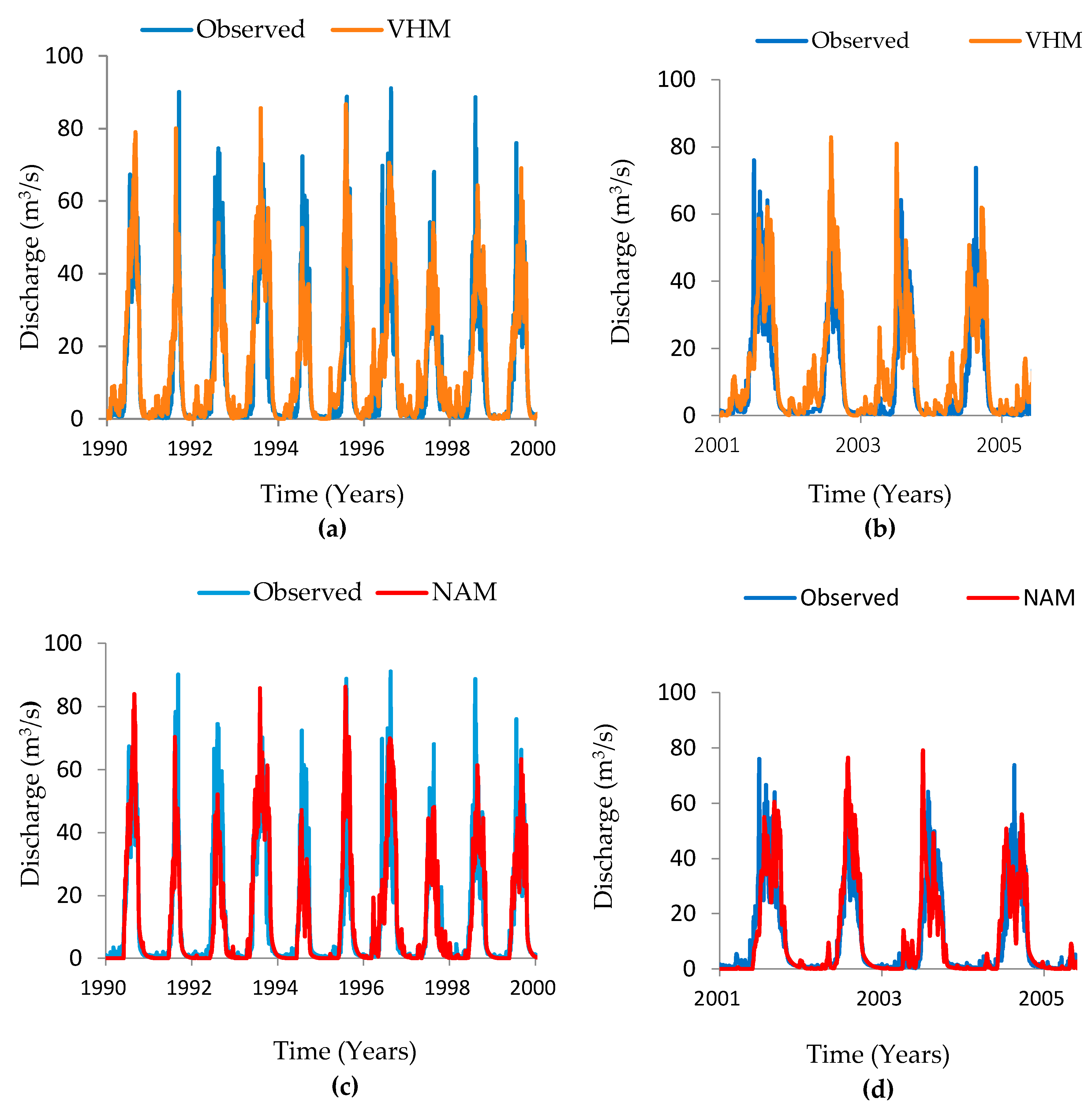
The catchment runoff is reproduced by the models in a reasonable way. Nevertheless, the VHM depicts slightly lower performances both statistically and graphically as compared to the NAM model which might be attributed to its sensitivity to the quality of rainfall data. A similar study [
19,
33], conducted on Grote Nete catchment in Belgium, demonstrated the lower performances of the VHM model as compared to the NAM and PDM conceptual rainfall runoff models, which is comparable to the result obtained for this study. In addition, the HBV, VHM and NAM models were applied to predict the streamflow of the Upper Blue Nile basin at ElDiem gauge station and found that the NAM showed better performances as compared to the VHM [
34]. It is clear that both the models reproduced the streamflow which was good in accordance to the observed flow. However, the overall results reflected that the NAM prediction of the streamflow was better than that of VHM. The low quality and low data availability might be possible obstacles for higher efficiency achievement in the data scarce region like the study catchment. Overall, the good agreement between the observed and simulated flow demonstrated by the two models indicates that the models can jointly allow hydrological simulation in the study catchment.


