Article

Evaluation and Bias Correction of CHIRP Rainfall Estimate for Rainfall-Runoff Simulation over Lake Ziway Watershed, Ethiopia

by
Demelash Wondimagegnehu Goshime
1,3,*,
Rafik Absi
2 and
Béatrice Ledésert
1
1
Laboratory of Geosciences and Environment Cergy (GEC), University of Cergy-Pontoise, 95000 Neuville Sur Oise, France
2
ECAM-EPMI Graduate School of Engineering, 95092 Cergy-Pontoise, France
3
EBI School of Engineering, 49 Avenue des Genottes, 95895 Cergy-Pontoise, France
*
Author to whom correspondence should be addressed.
Hydrology 2019, 6(3), 68; https://doi.org/10.3390/hydrology6030068
Submission received: 16 June 2019 / Revised: 28 July 2019 / Accepted: 6 August 2019 / Published: 9 August 2019

Abstract

:
In Lake Ziway watershed in Ethiopia, the contribution of river inflow to the water level has not been quantified due to scarce data for rainfall-runoff modeling. However, satellite rainfall estimates may serve as an alternative data source for model inputs. In this study, we evaluated the performance and the bias correction of Climate Hazards Group InfraRed Precipitation (CHIRP) satellite estimate for rainfall-runoff simulation at Meki and Katar catchments using the Hydrologiska Byråns Vattenbalansavdelning (HBV) hydrological model. A non-linear power bias correction method was applied to correct CHIRP bias using rain gauge data as a reference. Results show that CHIRP has biases at various spatial and temporal scales over the study area. The CHIRP bias with percentage relative bias (PBIAS) ranging from −16 to 20% translated into streamflow simulation through the HBV model. However, bias-corrected CHIRP rainfall estimate effectively reduced the bias and resulted in improved streamflow simulations. Results indicated that the use of different rainfall inputs impacts both the calibrated parameters and its performance in simulating daily streamflow of the two catchments. The calibrated model parameter values obtained using gauge and bias-corrected CHIRP rainfall inputs were comparable for both catchments. We obtained a change of up to 63% on the parameters controlling the water balance when uncorrected CHIRP satellite rainfall served as model inputs. The results of this study indicate that the potential of bias-corrected CHIRP rainfall estimate for water balance studies.

Graphical Abstract

1. Introduction

Rainfall-runoff modeling requires accurate rainfall input data. The accuracy of the rainfall input significantly influences the performance of hydrological models. However, accurate and consistent rainfall observations are limited in many regions, particularly in developing countries, due to limited rain gauge networks and density of deployment [1,2]. Satellite rainfall estimates (SREs) may serve as an alternative data source for model inputs, as they provide rainfall datasets at various temporal and spatial coverage, including ungauged basins [3,4]. Nevertheless, the results of previous studies indicate that SREs can be subjected to substantial biases [5,6,7]. Hence, it is necessary to either minimize or remove the bias before the SREs can be used in any subsequent applications.
SREs derive rainfall datasets from either passive microwave (PMW) or thermal infrared (TIR), or a combination of both [8]. PMW depends on the relationship between the radiance in the microwave channel and precipitation, such as Asian Precipitation Highly Resolved Observational Data Integration Towards Evaluation of water resources (APHRODITE; [9]). TIR estimate relies on cloud top temperature threshold values and is relatively available at high temporal resolutions. Examples of TIR include Global Precipitation Climatology Centre (GPCC; [10]), Climate Prediction Centre Morphing Technique (CMORPH; [11]), and Climate Hazards Group InfraRed Precipitation (CHIRP; [12]), among others. However, very few of these satellite products have been evaluated over eastern Africa [5,13,14].
Previous studies on validation and inter-comparison of satellite products indicate that they are subjected to systematic (i.e., bias) and random errors [5,15,16]. The sources of these errors may arise from an error in sampling, rain gauge data coverage, bias correction, and retrieval algorithms, among others. These studies have also shown that biases can be minimized or removed by applying a bias correction algorithm to compare with rain gauge data. A bias correction algorithm may vary from linear [17] to a multiple moment distribution matching [18] of a variable at a time. The selection of the bias correction method depends on the accuracy, the data requirement, and the hydrologic application that the bias-corrected dataset can be used in [5].
Bias corrections have been applied in a number of previous satellite studies, such as [5,7,19]. Yuan et al. [7] showed that linear bias correction applied to Global Precipitation Measurement (GPM) and Tropical Rainfall Measuring Mission (TRMM) effectively improved the streamflow simulations. Habib et al. [5] showed that applying space and time fixed bias correction schemes in CMORPH revealed improved runoff simulation. Yong et al. [20] indicated that a bias-corrected rainfall product as the model input instead of an uncorrected product revealed improved performance on rainfall-runoff simulation.
Several studies also reported that a hydrologic model parameter requires recalibration when satellite rainfall data replace rain gauge data as model inputs [16,21,22]. They indicated an increase of hydrological model performance when the model was calibrated using SREs rather than rain gauge data. However, Worqlul et al. [23] calibrated the hydrological model for gauge, uncorrected, and bias-corrected Multi-Sensor Precipitation Estimate-Geostationary (MPEG) rainfall inputs in the upper Blue Nile basin in Ethiopia. They found that calibration of the model using different rainfall inputs resulted in different parameter values. Yong et al. [6] showed the requirement of recalibrating sensitive parameters that control the hydrologic model using different rainfall inputs during the validation period. Similar findings were also reported in other studies such as [5,24]. It is expected that different inputs might affect model performance and require different sets of parameters. However, studies that incorporate model parameters and rainfall input uncertainties are limited. Furthermore, the results of error tolerance and propagation into hydrologic model prediction are not consistent and need further assessment.
In the Central Rift valley lakes basin, rain gauge stations are sparse and unevenly distributed. Furthermore, some of the available rain gauge networks are inadequate to simulate reliable rainfall-runoff modeling, mainly due to sparse spatial coverage, a short length of records, and substantial missing data. Hence, satellite rainfall estimates at high spatiotemporal resolution may help to overcome these shortcomings. Therefore, the evaluation of satellite rainfall product over Lake Ziway watershed is crucial to fill the data gap in water budget studies. Most of the previous studies in Ethiopia over other parts of the basin have been conducted using coarse-resolution satellite rainfall products. In the present study, we focus on the use of relatively high space–time resolutions (0.05° × 0.05°, daily) and Climate Hazards Group InfraRed Precipitation (CHIRP) satellite rainfall for rainfall-runoff simulation at Meki and Katar catchments.
The main objectives of this study are: (i) to evaluate the performance of CHIRP satellite product at different spatiotemporal scales, (ii) to assess the effect of gauge, uncorrected, and bias-corrected CHIRP satellite rainfall inputs on calibrated model parameters and the model performance on streamflow simulations. To achieve these objectives, we devised the following steps: first, CHIRP satellite estimate was compared with the rain gauge rainfall at various spatial and temporal scales using graphical comparison and different statistical measures. Next, a non-linear power bias correction method was applied to correct the CHIRP rainfall estimate using available rain gauge stations in the study area. Then, a semi-distributed Hydrologiska Byråns Vattenbalansavdelning (HBV) hydrological model was used to calibrate and simulate streamflow driven by gauge, uncorrected, and bias-corrected CHIRP satellite rainfall inputs at Meki and Katar catchments.
The CHIRP satellite was selected in this study due to its relatively high spatiotemporal resolutions and its availability at consistent time series matching the rain gauge data interval and the time step of the hydrological model used in this study. Although the performances of satellite products are highly variable in space and time, previous inter-comparison studies of satellite rainfall products over the eastern Africa region indicate that the CHIRP satellite rainfall product performance is slightly better than other products due to high spatiotemporal resolutions [13,25,26]. Hence, in this study, CHIRP was selected. The results of this study provide information for the product users regarding the applicability of the CHIRP rainfall product for estimating catchment runoff in data scarce regions. In the Lake Ziway area, this study can contribute to filling the data gap in water budget studies, which play a significant role for water resources development programs in the study area.

2. Study Area and Datasets
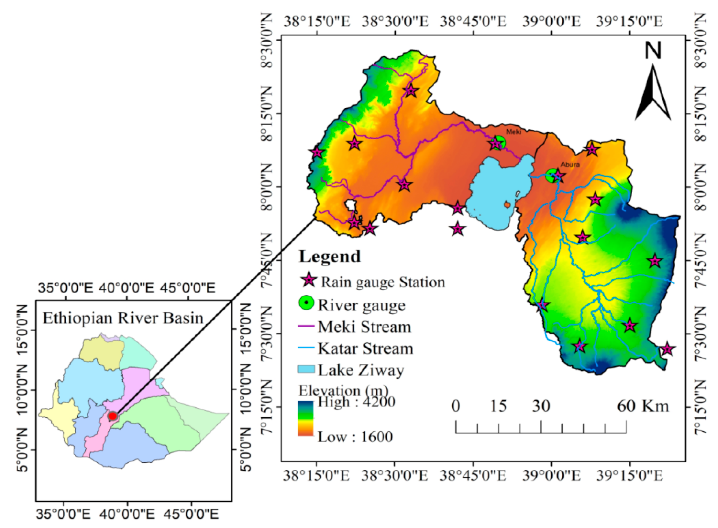
2.1. Study Area

The study area is Meki and Katar catchments, which are the major tributaries of Lake Ziway, located in the Central Rift Valley (CRV) lakes basin of Ethiopia with a total land surface area of 7022 km2. They are situated between 7.43°–8.58° N latitudes and 38.20°–39.25° E longitudes and drain the western and the eastern plateaus, respectively. The catchment area covers 6570 km2, of which the gauged catchment covers 5783 km2 (82% of the total Lake Ziway drainage area). The basin topography is characterized by mountainous terrain over east and west boundaries with an elevation ranging from 1600 to 4200 m above sea level (Figure 1).
Lake Ziway subbasin has tropical climate conditions with a mean monthly average temperature of the catchments ranging from 15.6 to 22.5 °C. The average annual rainfall of the catchment ranges from 740 to 1170 mm and from 750 to 1220 mm on the Meki and the Katar catchments, respectively. The rainfall in the rainy season (June to September) accounts for almost 60–70% of the total annual rainfall. Figure 1 shows the location of the study area with meteorological, river gauge and elevations indicated.

2.2. Rain Gauge Data

Daily rain gauge data for 20 meteorological stations from 1984 to 2014 were obtained from the National Meteorological Agency of Ethiopia. The dataset includes precipitation, maximum and minimum temperature, wind speed, humidity, and sunshine duration. Existing meteorological records in the study area are limited in both space and time. Data quality checks, homogeneity, and outlier tests were performed. After data screening, 14 rain gauge stations out of 20 stations were found to be reliable with relatively consistent records. In this study, these rain gauge datasets were used to simulate gauge-based streamflow and as a reference for comparison and bias correction of the satellite rainfall data.
Daily river discharge data are available for Meki and Katar Rivers, which are gauged at Meki and Abura town, respectively (Figure 1). Those data were obtained from the Ministry of Water, Irrigation and Electricity hydrology department database of Ethiopia. The data cover the period 1984–2000 at daily time steps. These observed data were used as a reference to compare and calibrate the hydrological model parameters as a result of different rainfall inputs.

2.3. Satellite Rainfall Data

The Climate Hazards Group InfraRed Precipitation (CHIRP) satellite product was used in this study. The CHIRP satellite was recently developed by the US Geological Survey (USGS) in collaboration with the Climate Hazards Group at the University of California. CHIRP uses TIR satellite rainfall estimates combined with the globally gridded satellite from National Oceanic and Atmospheric Administration (NOAA) to produce the rainfall dataset.
The CHIRP product has the potential to produce a near-real time satellite estimate at relatively high spatiotemporal resolution covering regions between 50° S to 50° N latitudes and all longitudes. The CHIRP rainfall datasets are available for the period 1981 to near-present at http://chg.geo.uscb.edu/data. In this study, the CHIRP rainfall estimate at daily and at 0.05° × 0.05° spatial scales for the period 1984-2014 are used. For detailed descriptions about the CHIRP product, refer to [12,27].

3. Methods

3.1. Evaluation of CHIRP Satellite Rainfall

We applied a graphical comparison plot and statistical measures to evaluate the performance of CHIRP satellite data at various spatiotemporal scales. First, we evaluated the CHIRP satellite product through visual inspection of scatter plots at catchment average daily and monthly scales. Then, the CHIRP satellite rainfall was quantitatively evaluated against rain gauge observations using five performances of statistical measures at point and catchment scales on a daily and a monthly basis. The selected performance statistical measures included Pearson correlation coefficient (CC), percentage relative bias (PBIAS), mean error (ME), mean absolute error (MAE), and root mean square error (RMSE). The CC indicates the agreement in terms of dynamics between the satellite estimate and the rain gauge observation. The PBIAS represents the relative systematic bias of the satellite rainfall from the rain gauge observation. The ME and the MAE provide information on average and magnitude of error, respectively. The RMSE measures the average absolute errors of satellite rainfall, with smaller values indicating the closure between the two datasets.
In addition to the numerical statistical measures, three categorical validation statistics were used to assess the performance of the satellite in rain intensity detection capability. These verification statistics included probability of detection (POD), false alarm ratio (FAR), and critical success index (CSI), following [6,19,25]. POD was used to assess the observed rain events that were correctly detected by the satellite. FAR represents the observed rain events that were incorrectly detected by the satellite. The CSI measured the overall correspondence between the satellite and the rain gauge occurrence of rain events. These categorical verification statistics referred to the skill of a satellite estimate for detection of observed rainfall events, taking into account a threshold value for the presence of rain or no rain to separate events at any time scale (e.g. daily, monthly, etc.). The metrics were derived from a contingency term in which the letters H, F, and M represent, respectively, hits (event forecasted to occur and did occur), false alarms (event forecasted to occur but did not occur), and missing (event forecasted not to occur but did occur). A threshold value of 1 mm day−1 in each grid cell and rain gauge station was assumed in this study, following [6,13,25]. The values of POD and CSI varied from 0 to 1, with a perfect score when a value of 1 registered with a value of 0 for FAR. The statistical measures were evaluated at various spatial (point, catchment) and temporal (daily, monthly) scales from 1985 to 2000. The equations for all numerical and categorical metrics along with their descriptions are summarized in Table 1.
To further assess the season variation between the satellite and the rain gauge, the mean monthly rainfall amounts of the respective datasets for Meki and Katar catchments were compared. The rain gauge rainfall was from an ensemble of 14 rainfall stations (6 for Meki and 8 for Katar catchments), and the satellite data were from 215 grid cells aggregated to mean monthly for both catchments. Then, the mean monthly rainfall pattern and the season rainfall difference for the rainy season (June–September) and the dry season (October–February) were compared between the two datasets.

3.2. CHIRP Satellite Bias Correction

We note that satellite rainfall estimates are subject to substantial systematic errors [5,6,7]. These errors may produce uncertainty in the hydrological model, which could result in under or overestimation of the simulated streamflow. Furthermore, model parameter values obtained using uncorrected SREs inputs into the model might not respond with reliable estimates of the watershed characteristics [28]. Therefore, biases in rainfall estimate must be corrected before it can be used as input into a hydrological model for streamflow simulation. In this study, the bias of the uncorrected CHIRP satellite estimate was corrected using the non-linear power transformation bias correction method [16,29]. The approach is based on matching the probability distribution function (such as mean, standard deviation, coefficient of variation) of the CHIRP with that of the rain gauge data. The equation reads:
P c = a P o b
where Pc is bias-corrected CHIRP rainfall, Po is original satellite-only (uncorrected) rainfall, and a and b are bias factors.
The values of bias factors were determined iteratively until the observed value matched with the CHIRP satellite by jointly arranging the whole daily data of both data sources for each month over the period 1985–2000. First, the bias factor (b) was estimated with a coefficient of variance of the satellite that matched with that of the rain gauge. Then, the bias factor (a) was determined by adjusting the mean of the satellite and the rain gauge datasets [30]. The bias factor at the selected 14 grid pixels was estimated at a minimum zero error objective function using the Excel Solver function available in the Microsoft Excel program. Then, the bias factors were applied on a monthly basis for the entire dataset. For other grid cells that did not contain rain gauge stations, the bias factors were interpolated using inverse distance weighted (IDW) methods. The bias-corrected areal CHIRP rainfall for the respective catchments was estimated using the Thiessen polygon from representative grid pixels and was then used as input in the hydrological model.
To verify the bias correction algorithm and to show the improvement obtained after bias correction, we applied a comparison of all statistical measures between daily bias-corrected satellite and rain gauge datasets. In addition, plots of cumulative distribution function (CDF) between gauge, uncorrected, and bias-corrected satellite rainfall at areal catchment average basis were compared for both Meki and Katar catchments.

3.3. HBV Hydrological Model

In this study, we applied the Integrated Hydrological Modeling System (IHMS) version 6.3 HBV rainfall-runoff model for streamflow simulation. The HBV model was selected in this study due to its proven performance over Ethiopian catchments [5,31,32,33,34]. The model also allowed us to divide the modeling domain into multiple sub-catchments, elevation, and land use zones. The climate and the hydrological input data for the simulation included daily rainfall, temperature, potential evapotranspiration, and river discharge. The catchment potential evapotranspiration was estimated by the Penman–Monteith [35] method from eleven meteorological stations. The areal potential evapotranspiration over the catchment was computed using the Thiessen polygon method from representative stations and then used as input of the hydrological model.
The HBV model consists of subroutines for precipitation, soil moisture accounting, runoff generation, and routing routine. Precipitation routines ensure that precipitation is either simulated as snow or rain. In the Lake Ziway catchment area, precipitation was simulated only in the form of rainfall. The soil moisture routine controls the formation of runoff based on FC, BETA, and LP parameters. FC is the field capacity at maximum soil moisture storage. BETA accounts for non-linearity of indirect runoff from the soil layer. LP is the limit of potential evaporation, which indicates the soil moisture value above which actual evapotranspiration reaches its potential value. The runoff generation routine transforms excess water from the soil moisture zone to runoff. The relation of runoff routine is expressed by:
Q u = K u · U Z ( 1 + A l f a )
Q L = K 4 · L Z
where Qu and QL are the runoff components from upper and lower reservoir zones, respectively; Ku is the recession coefficient in the upper zone, and K4 is the recession coefficient in the lower zone; UZ and LZ are the actual storages in the upper and the lower zones, respectively; Alfa is a measure of the non-linearity of the flow in the upper reservoir zone. The total sum of Equations (2) and (3) yields the amount of the streamflow generated at the catchment outlet.
In this study, the parameters used for model calibration were selected from previous studies [23,32,34]. Accordingly, eight model parameters (FC, BETA, LP, K4, Khq, Alfa, CFLUX, and PREC) were selected for model calibration. The ranges and the initial values of these parameters were defined as recommended by [36]. A detailed description of the HBV model is available in [36,37]. Table 2 presents the summary of the descriptions, the value ranges (minimum–maximum), and the initial values of the selected calibrated parameters.

Model Calibration and Evaluation

In this study, the HBV model was calibrated and verified for an independent validation period using three rainfall datasets. These were gauge, uncorrected, and bias-corrected CHIRP satellite rainfall data. For each dataset, the HBV model parameters were calibrated by comparing the simulated streamflow against the observed discharge data at Meki and Katar river gauge stations. To aid model calibration, sensitive model parameters were identified based on the model performance objective function values. For comparison of sensitive calibrated model parameter values over a common scale, we normalized between the minimum and the maximum value range. A manual model calibration by changing one parameter value at a time within the allowable range was applied to obtain the optimal parameter values. Then, the most sensitive parameters that control runoff volume were calibrated first, followed by the routing parameters. The model calibrations run from 1986–1991 periods for Meki and Katar catchments. Then, the model was validated for an independent period from 1996–2000 for both catchments. The 1984–1985 periods was used as the warm-up period for initializing the levels of the model reservoirs. Note that substantial data records from 1992–1995 are missing, hence this period was not considered either for calibration or validation.
The simulated streamflows from the three datasets were compared to the observed streamflow to assess the model performance for rainfall-runoff simulations. The model performance was evaluated using Nash–Sutcliffe efficiency (NSE) and relative volume error (RVE) in addition to visual inspection of the simulated hydrograph. NSE measures the agreement between the simulated and the observed hydrographs. RVE measures the average volume difference between the simulated and the observed streamflow. The equations for both objective functions are:
NSE = 1 i = 1 n ( Q sim , i Q obs , i ) 2 i = 1 n ( Q obs , i Qobs ¯ ) 2
RVE = [ i = 1 n ( Q sim , i Q obs , i ) i = 1 n Q obs , i ] × 100 %
where Qsim and Qobs represent simulated and observed streamflow, respectively (m3s−1), and the over-bar symbol denotes the mean of the statistical values; i is the time step; n is the number of a sample size of a paired data time series. NSE has a dimensionless value ranging from −∞ to 1.0, 1.0 corresponding to a perfect fit. RVE ranges between −∞ and ∞, but the model performs best when a value of 0 is obtained. A value between +5% and −5% indicates that a model performs very well while a value between ±5 and ±10% indicates that a model has reasonably good performance.

4. Results and Discussion

4.1. Evaluation of CHIRP Data at Multiple Spatiotemporal Scales

The scatter plots in Figure 2 compare the satellite products (uncorrected) and the gauge rainfall at daily and monthly time scales for Meki and Katar catchments. The data plots are shown for areal average at the catchment level covering the period from 1985 to 2000. There was wide scatter for both catchments, indicating strong disagreement between the uncorrected and the rain gauge observation at daily time scales. Few data points were spread along the 45° degree line, indicating a poor correlation between the two datasets with correlations of 0.37 and 0.40 for Meki and Katar catchments, respectively. On average, rainfall amounts up to 45 mm per day were missed by CHIRP for both catchments. However, for monthly time scale comparison, more data points were close to the 45° degree line, indicating a better agreement of the satellite estimate with the rain gauge observation. This phenomenon might be related to the performance of the CHIRP satellite estimate at seasonal time scales.

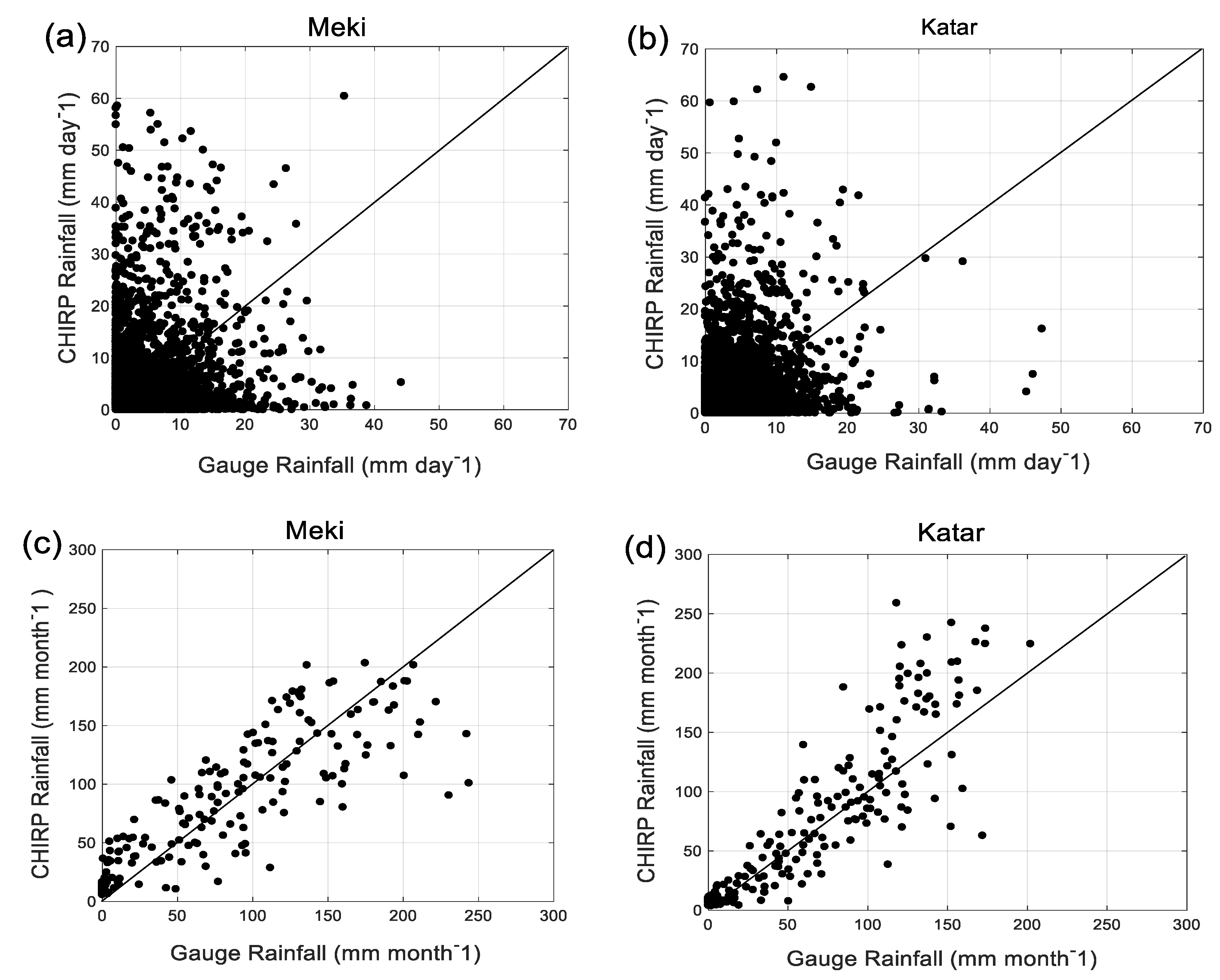
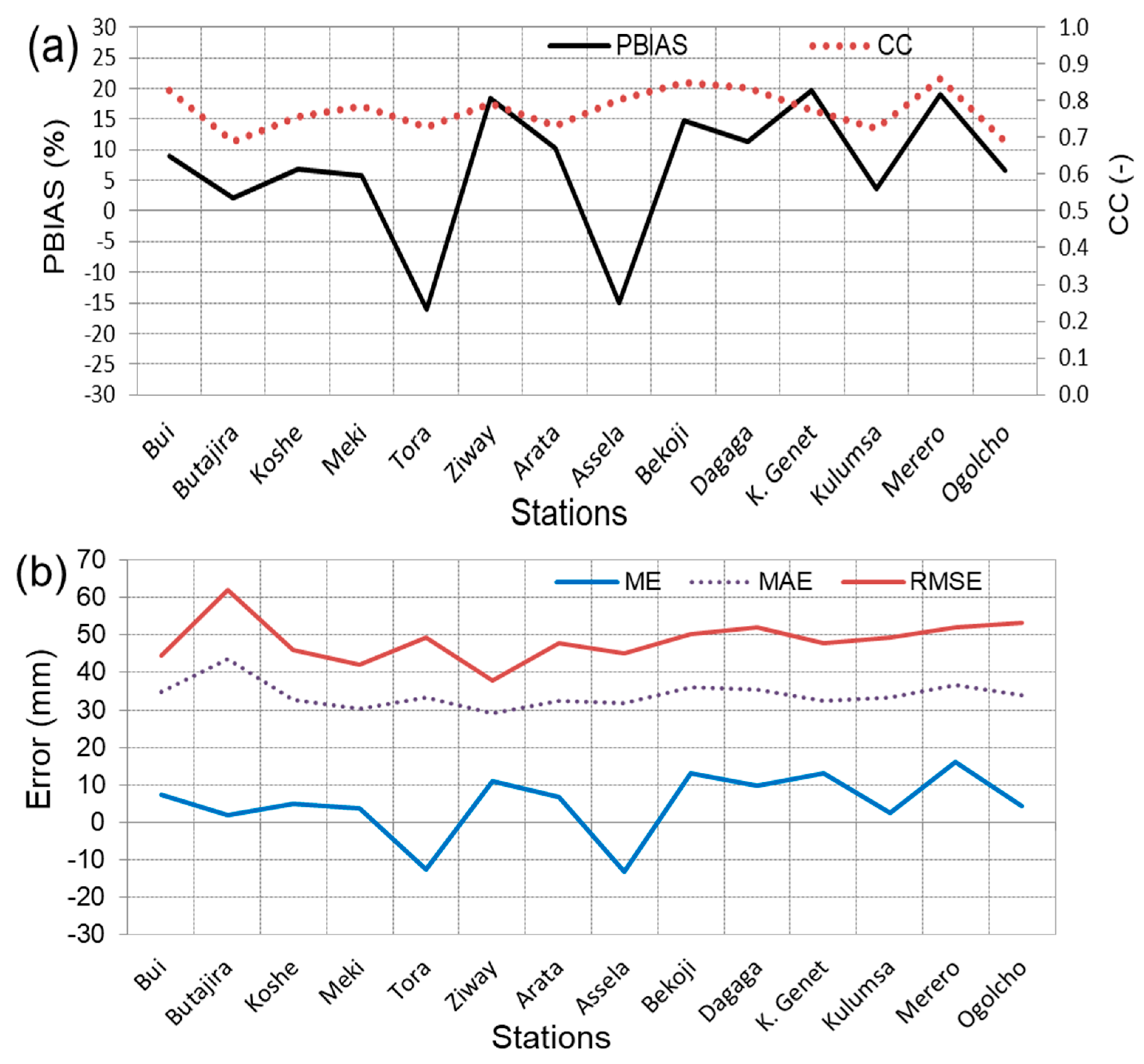
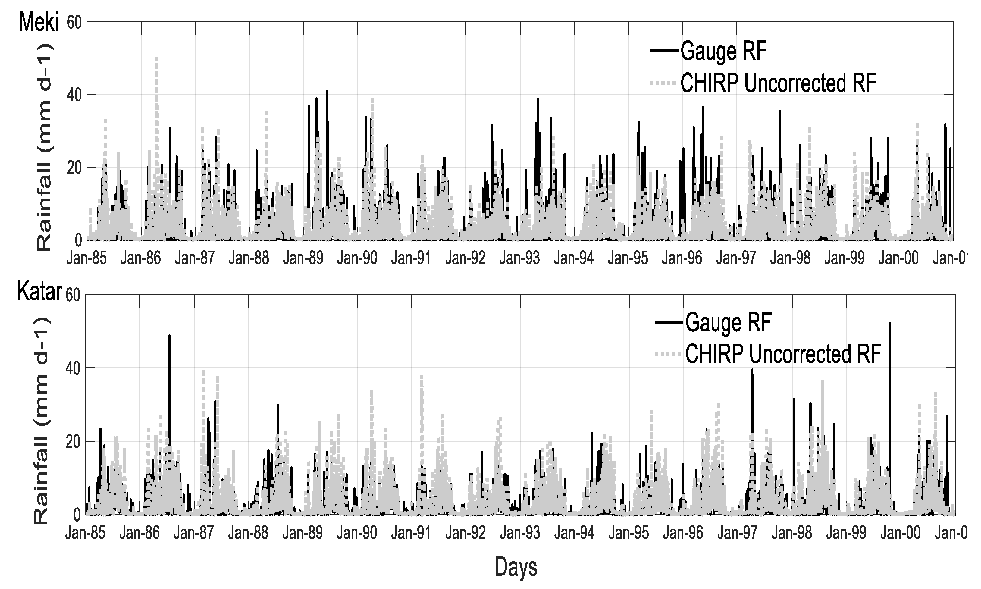
4.1.1. Point-Scale Daily Rainfall Comparison

The performance of the CHIRP satellite estimate was evaluated by comparing it with 14 rain gauge stations based on statistical measures at daily scales from 1985 to 2000. We selected six stations (i.e., Bui, Butajira, Koshe, Meki, Tora, and Ziway) that are located at Meki catchment and eight stations (i.e., Arata, Assela, Bekoji, Dagaga, Ketera Genet, Kulumsa, Merero, and Ogolcho) from Katar catchment to evaluate the performance of the CHIRP satellite estimate.
Table 3 shows the result of both numerical and verification statistical measures obtained by comparing each grid with rain gauge stations at daily time scales. We note that CHIRP showed poor performance in the majority of the stations at a daily time step. The CC values ranged from 0.17 to 0.4 (less than 0.5), which indicated a poor correlation of the CHIRP satellite with gauge rainfall. The results show that the correlation varied from one station to another—lower at Arata, Tora, and Ogolcho stations and relatively higher at Merero, Bekoji, and Dagaga stations. This phenomenon is related to the performance of the CHIRP satellite at lower and higher rainfall regions, respectively.
The PBIAS result showed that CHIRP overestimated in most of the stations except for underestimations in Tora (−15%) and Assela (−16%), where they revealed a negative PBIAS (Table 3). The possible reason for this could be that both stations are located in relatively higher elevation regions as compared to the other stations. Dinku [3] and Khandu et al. [26] reported similar results over Eastern Africa and Bhutan, respectively. The mean error revealed to be relatively smaller compared to other performance measures. Butajira and Kulumsa stations showed a smaller error with relatively similar altitude locations. In terms of MAE and RMSE, most of the stations contained similar error magnitude.
The categorical measures also showed POD values ranging from 0.51 to 0.69, indicating that the CHIRP satellite correctly detected the observed rain events by a maximum of 69% over the study area (Table 3). According to Table 3, the FAR values for most of the rain gauge stations were greater than 0.5, implying that over 50% of observed rain events were incorrectly detected by the satellite. Furthermore, the values of CSI registered smaller values less than 0.5 in all the rain gauge stations and the corresponding grid cells, indicating the error of the CHIRP satellite with the rain gauge dataset. It is in this aspect that the application of bias correction is necessary to remove the bias before it can be used for streamflow simulation.

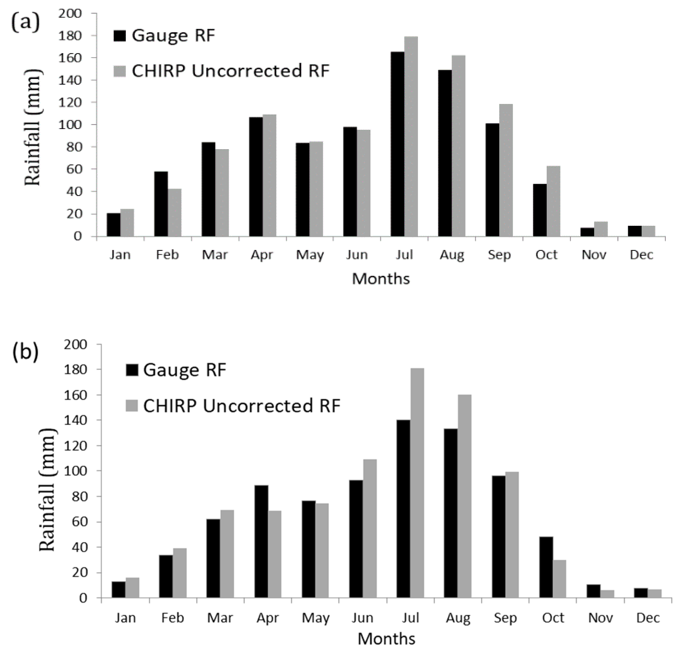
4.1.2. Point-Scale Monthly Rainfall Comparison

Figure 3 shows the selected statistical measures for 14 rain gauge stations compared against the grid cells at a monthly period from 1985 to 2000. The figures illustrate that the agreement between the CHIRP satellite and the rain gauge stations significantly improved when the daily data were aggregated to a monthly scale. We note that the correlations for all stations were increased above 0.5. The probable reason for this improvement was because the CHIRP satellite might have captured the temporal pattern of seasonal rainfall over the study area.
The PBIAS for monthly basis remained the same as the daily scale. However, higher values of MAE and RMSE error magnitude revealed up to 44 and 62 mm, respectively, indicating the error between the satellite and the rain gauge stations. In general, at a monthly time scale, the CHIRP satellite performed relatively poorly at Ogolcho, Butajira, Arata, and Tora stations as compared to other stations, which showed relatively lower CC and higher values of PBIAS, ME, MAE, and RMSE (Figure 3).

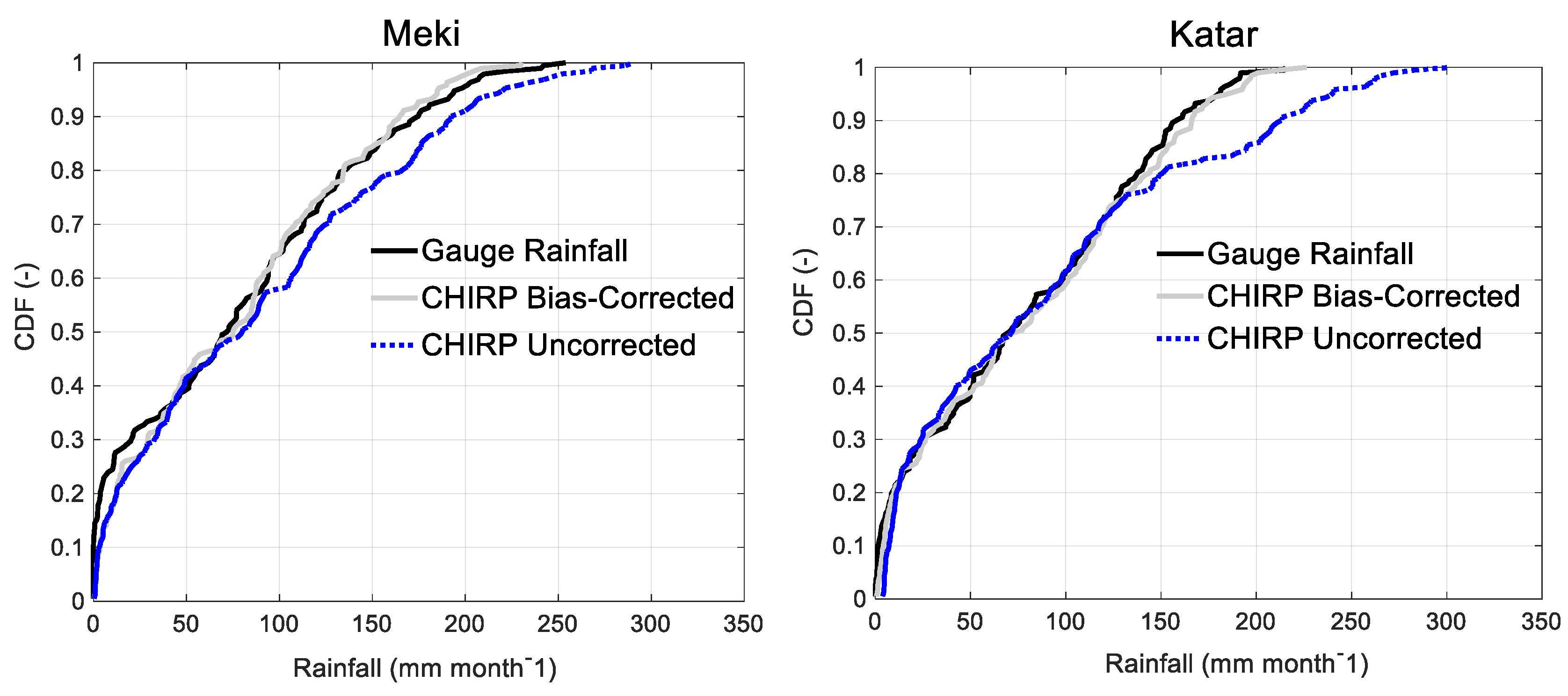
4.1.3. Catchment-Scale Rainfall Comparison

To evaluate the performance of the CHIRP satellite at the catchment scale, the comparison was performed between daily areal average rainfall from the rain gauge and the satellite. Figure 4 shows the daily rainfall time series comparison of the rain gauge and the satellite at Meki and Katar catchments. The figure indicates that the CHIRP satellite rainfall better captured the temporal variations of the daily gauge rainfall at both catchments. However, the agreement for Katar catchment was better than for Meki catchment, as there were some observed extreme peaks not effectively captured by the satellite. This phenomenon was partly attributed to the sparse rain gauge network in Meki catchment compared to Katar.
Table 4 shows the comparison of the CHIRP satellite with the gauge counterparts at a daily catchment level. At a daily time scale, the CHIRP satellite showed poor correlation with the rainfall from the rain gauges for both catchments, with CC values of 0.37 and 0.40 for Meki and Katar catchments, respectively. PBIAS results showed that CHIRP overestimated at Meki with a positive bias of 3.8% and underestimated over Katar catchment with a negative bias value of −2.0%. The ME revealed a smaller value of 0.1 mm for Meki and 0.3 mm for Katar catchment. The magnitude of the error in terms of RMSE and MAE revealed almost similar error values for both catchments.
The POD results showed that 62% and 70% of the rain gauge rainfall events were correctly detected by the CHIRP for Meki and Katar catchments, respectively. The observed rainfalls that were not detected by the satellite reached up to 39% for Meki and 25% for Katar catchments (Table 3). The CSI resulted in 0.45 and 0.50 for Meki and Katar catchments, respectively, which measured the overall correspondence of the satellite and the rain gauge occurrence of rain events. Overall, the results showed relatively better performance for Katar than Meki catchment in terms of all statistical measures. Possible reasons for the better performance of Katar catchment were due to a relatively higher rainfall in the region and a larger number of rain gauge networks compared to Meki catchment. Khandu et al.’s study [26] also indicated that the CHIRP satellite performed slightly better in the higher rainfall region over Bhutan.
To further evaluate the seasonal difference between the two datasets, the mean monthly rainfall patterns of the CHIRP satellite and the rain gauge stations for Katar and Meki catchments from 1985–2000 are shown in Figure 5. The results revealed that the mean monthly rainfall better captured the pattern of rainfall for the rain gauge. However, it did not satisfactorily capture the gauged rainfall amount, especially for the rainy season (June–September). The highest difference between the two datasets was in the month of July, with values of 17 and 41 mm for Meki and Katar catchments, respectively. During the dry season (October–February), the highest difference of the satellite from the rain gauge was −16 mm for Meki and −19 mm for Katar catchments. This clearly showed that an overestimation of the CHIRP satellite estimate during wet seasons and an underestimation during dry seasons. These results showed the magnitude of the CHIRP satellite bias varied at seasonal scales over the study area.

4.2. CHIRP Satellite Bias Correction

We note that the CHIRP satellite has biases at various spatial and temporal scales. Furthermore, several studies have also indicated that SREs must be corrected for use in various applications [5,7,38,39]. In this study, we applied a non-linear power bias correction approach (described in Section 3.2) using Equation (1) to estimate bias-corrected CHIRP satellite rainfall datasets. The bias factors were determined by comparing satellite and rain gauge data with established constraints and objective functions. The results from an ensemble of 14 rain gauge stations indicated that bias factors varied at spatial and temporal scales for both catchments. The results showed that, on average, the bias factor a varied from 0.01 to 1.72 and b from 1 to 4 over the two catchments.
Table 5 shows the statistical measures between the daily bias-corrected CHIRP estimate and the rain gauge after applying bias correction. Improvements were found in all numerical statistical measures (CC, PBIAS, ME, MAE, and RMSE) and categorical statistics (POD, FAR, and CSI). This indicated better performance and improvement after bias correction of the CHIRP rainfall estimate as compared to the uncorrected CHIRP estimate. Hence, the bias-corrected CHIRP satellite effectively reduced the bias of the original uncorrected CHIRP rainfall. The POD result showed that more than 76 and 82% of the observed rainfall events from the rain gauge were correctly detected by the bias-corrected CHIRP satellite in Meki and Katar catchments, respectively. Moreover, smaller values of FAR and larger CSI values were registered after bias correction of the CHIRP satellite rainfall for both catchments, indicating better agreement of the bias-corrected satellite estimate and the rain gauge observation over the study area.
Figure 6 presents the cumulative distribution function (CDF) plot between gauge, uncorrected, and bias-corrected CHIRP rainfall at a monthly average catchment scale from 1985 to 2000. The figure indicates that the bias-corrected CHIRP rainfall estimate was very close to the rain gauge at all rainfall measurement values except for low rainfall (less than 50 mm month−1) for Meki catchment. This phenomenon was mainly related to the sparse rain gauge network in Meki catchment and the uncertainty of the bias-correction method for the satellite rainfall estimate. A similar result was reported by previous studies of Ayehu et al. [25] over the upper Blue Nile basin in Ethiopia. Overall, the bias-corrected satellite rainfall very well predicted the cumulative gauge rainfall distribution. It showed significant improvement and a better correlation between the satellite and the rain gauge data when the CHIRP data were corrected. However, the uncorrected CHIRP satellite data were below the rain gauge data at most of the data points as compared to the bias-corrected data for both catchments. Therefore, the results indicated that bias-correction significantly lowered the error of the CHIRP satellite rainfall estimate.

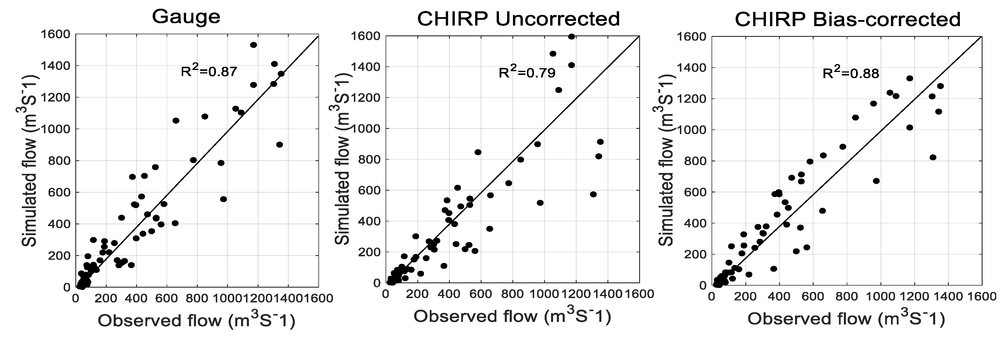
4.3. Model Calibration and Evaluation

For each calibration run, the HBV model parameter was independently calibrated for different rainfall inputs by comparing each simulated streamflow time series with the observed streamflow. First, the sensitive model parameter was evaluated. The result indicated that the parameters controlling the water balance (BETA, FC, and LP) were found to be the most sensitive parameters, while routing parameters (K4 and Khq) were relatively less sensitive. Parameters Alfa, PERC, and CFLUX were the least sensitive model parameters. Worqlul et al. [23] reported similar results at Gilgel Abbay and Gumara watersheds in Ethiopia. Next, we assessed how the calibrated model parameters and the performance of the hydrological model were affected as a result of gauge, uncorrected, and bias-corrected CHIRP satellite rainfall inputs at Meki and Katar catchments from 1986–1991. We chose to use the observed streamflow as a reference to compare the simulated streamflow for the three rainfall inputs.
Figure 7 shows the simulated and the observed daily hydrograph at Meki gauge stations for calibration periods (1986–1991) as input from the gauge, the uncorrected, and the bias-corrected CHIRP satellite rainfall datasets. For all rainfall inputs, the simulated streamflow captured the pattern of the observed hydrograph. However, it was reasonably captured over the simulation period when the model was forced by bias-corrected CHIRP satellite rainfall. We note that the simulated peaks for the three rainfall datasets were lower than the observed peaks. This phenomenon was partly attributed to poor quality and sparsely distributed rain gauge networks over Meki catchment. The uncertainties of bias-correction of the satellite estimate were also possible reasons for poor capture of the peak discharge during the model driven by bias-corrected satellite rainfall. Figure 5 shows that CHIRP overestimated during most of the rainy season for the two catchments. However, this did not cause higher streamflow to be simulated. This indicated that some of the excess rainfall might have been stored in the soil moisture zone and behaved as a low-pass filter instead of generating runoff. A similar finding was also reported by Habib et al. [5] for Gilgel Abbay catchment.
Table 6 presents the calibrated model parameter values and the model performance of Meki catchment using gauge, uncorrected, and bias-corrected CHIRP satellite rainfall inputs. The results showed that the bias-corrected CHIRP satellite significantly improved the performance of streamflow flow simulations. In terms of objective functions, the simulations for the gauge and the bias-corrected CHIRP satellite resulted in comparable values. In Meki catchment, the gauge and the bias-corrected CHIRP satellite indicated NSE of 0.67 and 0.71, respectively, and an RVE of less than 5%. This indicated good performance of the HBV model in the study area for the two datasets. Furthermore, the calibrated model parameter values for gauge and bias-corrected were also very close, except for a few routing parameters such as K4, Khq, and Alfa.
The calibrated model parameter values were within the allowable range for all rainfall inputs. However, parameter values were significantly changed when the uncorrected CHIRP served as model input. The model performance simulated using the uncorrected CHIRP satellite revealed lower performance than the gauge and the bias-corrected models in terms of both NSE and RVE. In Meki catchment, the CHIRP satellite rainfall overestimated gauge rainfall by 3.8% at a catchment average scale (Table 4) and underestimated by 16% at Tora station (Table 3). The simulated streamflow when the uncorrected CHIRP satellite rainfall served as model input revealed underestimation of runoff volume by 13.5% (Table 6). The results indicated that overestimation bias in rainfall translated into underestimation in streamflow. This was related to a proportion of the rainfall inputs in the model being stored as excess rainfall in the reservoir instead of contributing to streamflow simulations.
This study also indicated that rainfall input errors were compensated using independent model calibration by changing the best-fitted parameter values. The best-fitted parameter values were significantly varied when the uncorrected CHIRP rainfall served as model input as compared to the gauge rainfall. We note that parameters that control baseflow, water balance, and routing noticeably varied. For instance, in the HBV model, parameter FC (field capacity) corresponded to the maximum soil moisture storage, which affected the runoff volume. A higher value of FC tends to generate higher total runoff. Table 6 shows that the calibrated parameter FC increased from 850 mm for the gauged-based simulation to 960 mm for the uncorrected CHIRP satellite rainfall. This indicated that soil moisture storage should have been increased at least by 110 mm to minimize the reduction in runoff as a result of rainfall difference.
Parameters Khq and Alfa also related to peak flows, and a higher value of these parameters resulted in higher peaks and more dynamic response in the hydrograph. A value of Khq increased from 0.02 in the gauge-based model simulation to 0.2 in the uncorrected CHIRP rainfall estimate to cope with few extreme flows. The parameters related to baseflow and recession parameters (PERC, K4, and CFLUX) were increased to respond to the catchment characteristics for the uncorrected CHIRP rainfall inputs. Hence, this study indicates that different rainfall inputs result in different calibrated model parameters.
Figure 8 presents the monthly time series scatter plots between the observed and the simulated streamflows for gauge, uncorrected, and bias-corrected CHIRP satellite rainfall datasets at Meki catchment. When the model was driven by the gauge and the uncorrected CHIRP rainfall estimate, few streamflow data points were scattered and revealed a lower correlation than the bias-corrected CHIRP estimate. Part of this scatter may have been attributed to the uncertainty of the rain gauge data and the bias of the uncorrected CHIRP satellite estimates. However, the bias-corrected CHIRP estimate had less scatter and higher correlation as compared to the gauge and the uncorrected CHIRP estimates. These results indicated improvement of streamflow simulation after bias correction at the monthly time scale.
Figure 9 shows a comparison of the simulated and the observed streamflows for the calibration period (1986–1991) using gauge, uncorrected, and bias-corrected CHIRP rainfall inputs at Katar gauge stations. The figure demonstrates that observed peaks were better captured in most of the simulation period by the simulated streamflow when the model was forced by gauge and bias-corrected CHIRP satellite rainfall estimates. However, the pattern and some observed peaks were not satisfactorily captured by the simulated hydrograph when the uncorrected CHIRP served as model input. This was mainly because excess rainfall might have been stored in different reservoirs zones instead of generating runoff in addition to the underestimation of higher rainfall values of the rain gauge by the CHIRP rainfall (Figure 5). As compared to Meki, in Katar, the simulated peaks in the gauge-based simulation better captured the observed peaks, similar to the bias-corrected satellite rainfall inputs. This was mainly related to the relatively larger number of rain gauge stations used to simulate the gauge-based streamflow and evaluate bias correction at Katar catchment.
Table 7 presents the calibrated model parameter values and the model performance of Katar catchment using gauge, uncorrected, and bias-corrected CHIRP rainfall inputs. In Katar catchment, the gauge and the bias-corrected rainfall resulted in comparable model performances with NSE of 0.78 and 0.80, respectively, and an RVE of less than 5%. Similarly, the calibrated model parameter values for gauged and bias-corrected CHIRP were closer, except FC, Khq, and BETA parameters. However, when the uncorrected CHIRP satellite was used to derive the simulation run, most sensitive parameters were significantly varied. The model performance deteriorated with NSE of 0.70 and −13.4% RVE as compared to the gauge and the bias-corrected CHIRP rainfall inputs. This result was mainly related to underestimation of the CHIRP satellite estimate at a catchment average level (PBIAS −2%, Table 4) and point scales (PBIAS −20%, Table 3).
In Katar catchment, the best-fitted model parameters also remained within the allowable parameter range for all rainfall inputs. However, there were significant differences in the calibrated model parameter values when the uncorrected CHIRP rainfall served as model input. Parameters that control the water balance (FC, BETA, and LP), the routing parameters (Khq and K4), and the baseflow parameter (PERC) showed significant change during uncorrected CHIRP inputs. For instance, FC increased from 860 mm in the gauge rainfall input to 930 mm in the uncorrected CHIRP input. The recession (Khq and K4) and the percolation (PERC) parameters were also changed during the uncorrected CHIRP rainfall input. Overall, when the uncorrected CHIRP rainfall input replaced the calibration process, changes up to 63% and 55% were obtained in water balance and routing parameters, respectively, as compared to the rain gauge rainfall. Hence, this study shows that common optimized parameter values could not be achieved for different rainfall inputs over the study area. Therefore, the biases of streamflow simulation are not only derived from rainfall estimates but also the uncertainty in the hydrological model parameters as a result of different rainfall inputs.
Figure 10 shows the monthly time series scatter plots between the observed and the simulated streamflows for gauge, uncorrected, and bias-corrected CHIRP satellite rainfall datasets at Katar catchment. The scatters for streamflow simulated using the gauge and the uncorrected CHIRP rainfall estimates were higher than the bias-corrected CHIRP rainfall, implying the bias correction of the CHIRP rainfall estimate effectively improved the streamflow simulation.
The calibrated process was verified through validation for an independent period from 1986–2000 for the three rainfall inputs at Meki and Katar gauge stations. Note that we did not recalibrate the model for different rainfall inputs during validation. We used calibrated model parameters of the respective rainfall inputs in all model simulations. Figure 11 compares the daily observed and the simulated streamflows for Meki and Katar catchments simulated by gauge, uncorrected, and bias-corrected CHIRP satellite rainfall. The figure illustrates that, for both catchments, the simulated streamflows better captured the patterns of the observed hydrographs for all rainfall inputs, except for a slight underestimation of observed peaks.
The model performance deteriorated slightly in the validation period as compared to the calibration period for all rainfall inputs. The model performance for both stations indicated acceptable results, with NSE greater than 0.70 and RVE less than 5% when the model was forced by gauge and bias-corrected CHIRP satellite rainfall. However, when the uncorrected CHIRP satellite served as model input, the model performance significantly deteriorated, with NSE of 0.64 and −4.96 RVE for Meki (Table 6) and NSE of 0.70 and −16.8% RVE for Katar catchment (Table 7). This indicated that systematic error (biases) of the CHIRP satellite propagated through the HBV model in the streamflow simulations.
This study indicated that, for both catchments, the bias-corrected CHIRP satellite simulation performed slightly better than the gauge-based simulation. Such results could be partly attributed to sparsely distributed rain gauge networks over the study area and the availability of CHIRP satellite data at relatively high spatiotemporal scales. Similar results have been reported in other satellite studies by [7,21,22,40], which they found an increased performance of the hydrological model when the model was calibrated using SREs rather than gauge rainfall. Therefore, this study suggests that bias-corrected CHIRP satellite rainfall can be used as a potential alternative data source for water budget studies in Lake Ziway watershed.

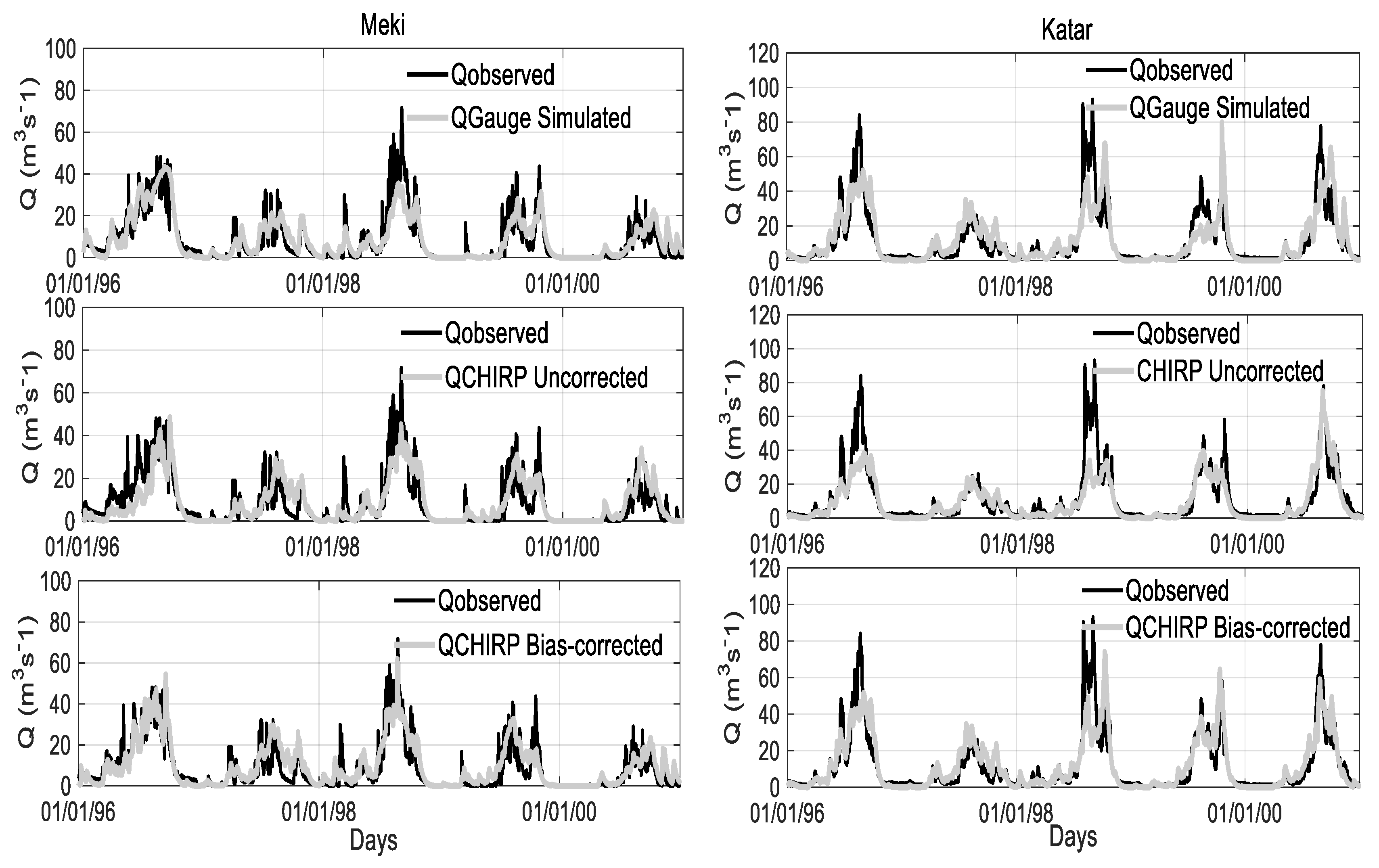
4.4. Evaluating the Value of Bias Correction on Streamflow

To evaluate the contribution of bias correction on streamflow and error propagation, we used the calibrated model parameter with gauge rainfall to simulate streamflow using the uncorrected and the bias-corrected CHIRP rainfall estimates. This helped to minimize the uncertainty related to model parameters. To offset the effect of rainfall input errors, gauge-based simulated streamflow was used as a reference for comparison and to quantify the model performance objective functions. In this study, we followed Habib et al.’s [5] approach, who assessed the effect of CMORPH bias correction on streamflow of Gilgel Abbay catchment. To quantify the magnitude of error propagation in streamflow simulation, rainfall bias (BIAS) and relative volumetric error (RVE) performance measures were used. The rainfall bias (BIAS) was calculated as a ratio of the total sum of the satellite and gauge rainfall, and the RVE was calculated using Equation (5).
Table 8 shows the rainfall bias and the RVE for the uncorrected and the bias-corrected CHIRP satellites compared with the gauge-based estimation. For Meki catchment, the uncorrected CHIRP satellite rainfall amount was smaller by 18% (BIAS = 82%, Table 8) than the gauge rainfalls, which resulted in a 17% reduction in streamflow volume. In Katar catchment, the rainfall difference was −16% (BIAS = 84%, Table 8), which contributed 11% in streamflow volume difference. However, after bias correction, the error propagation significantly reduced. The bias obtained between the bias-corrected CHIRP and the gauge-based was smaller than the uncorrected CHIRP satellite. After applying the bias-corrected CHIRP rainfall estimate, the rainfall bias was reduced to 4% (BIAS = 96%, Table 8) and translated to only 5% in streamflow bias in Meki catchment, whereas 10% rainfall bias (BIAS = 90%, Table 8) translated to 3% in streamflow volume difference in Katar catchment. The results indicated that the bias in the CHIRP satellite rainfall was translated through the HBV model in streamflow simulations. Table 8 clearly shows that the bias correction added value to the satellite estimate by effectively reducing the error magnitude in rainfall and streamflow simulations. Habib et al. [5] and Yuan et al. [7] reported similar results over Ethiopian and China basins, respectively.

5. Conclusions

Satellite rainfall estimates are subject to substantial systematic biases. However, only a few studies have been conducted over eastern Africa that incorporate uncertainties of the satellite estimate in streamflow simulations. In this study, we evaluated the performance and the bias correction of the Climate Hazards Group InfraRed Precipitation (CHIRP) satellite rainfall for rainfall-runoff simulation at Meki and Katar catchments. The study is unique, as it considers the performance of the CHIRP satellite at various spatiotemporal scales and contains a hydrological assessment of this product for rainfall-runoff modeling. We also evaluated the effect of gauge, uncorrected and bias-corrected CHIRP satellite rainfall inputs on calibrated model parameters and model performance on streamflow simulations using the HBV hydrological model. The results of this study contribute to guiding satellite product users in the applicability of the CHIRP satellite product for rainfall-runoff simulations. The main conclusions drawn from the result of this study are as follows:
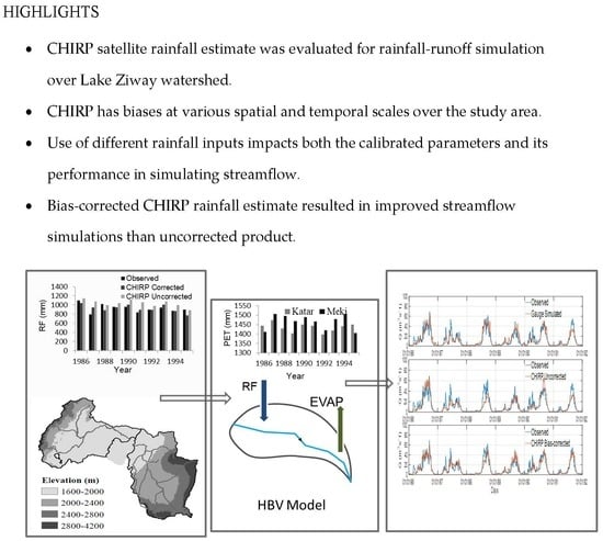
  • The results showed that the CHIRP satellite rainfall had biases at various spatial and temporal scales over Lake Ziway watershed. CHIRP had PBIAS ranging from −16 to 20% and lower correlation at a daily time step with the rain gauge data. Overall, CHIRP performance better improved at monthly and areal catchment scales.
  • We found comparable calibrated model parameters and model performances for the gauge and the bias-corrected CHIRP satellite rainfalls in simulating daily streamflow of the two catchments. However, calibrated model parameters significantly changed when the uncorrected CHIRP rainfall input served as model input. Changes up to 55% and 63% were obtained for water balance and routing controlling parameters, respectively, as compared to the gauge-based simulations. Hence, this study shows that common optimized parameter values could not be achieved for different rainfall inputs over the study area.
  • The simulated streamflow better captured the observed hydrographs when using the bias-corrected CHIRP satellite rainfall input compared to the uncorrected CHIRP satellite. We note that biases in satellite rainfall inputs were translated to simulated streamflow through the HBV hydrological model. The application of non-linear bias correction effectively reduced the rainfall bias and revealed improved streamflow simulation compared to the uncorrected product.
In general, this study shows that the bias-corrected CHIRP rainfall estimate can serve as an alternative data source in rainfall-runoff simulations for water budget studies. The study also suggests that bias correction is necessary to improve the performance of the satellite rainfall for accurate estimation of the hydrological response of the watershed. Future studies should incorporate a comparison of various bias correction algorithms to further explore the reported changes.

Author Contributions

All authors initiated the original idea of the study and fully contributed to analysis and interpretation of the results. D.W.G. was responsible for data acquisition, model setup, and calibration and to draft the manuscript. R.A. and B.L. edited the draft manuscript and supervised the research work. All authors read and approved the final manuscript.

Funding

This research was financial supported by the Ministry of Water, Irrigation and Electricity of Ethiopia (MoWiE) and the Article processing charge (APC) was funded by Cergy-Pontoise University Foundation. The authors gratefully acknowledge both institutes for the financial support of this study.

Acknowledgments

This study is part of Ph.D. research of the first author in Ethio-France sandwich program coordinated by France Embassy of Ethiopia and Campus France. Authors gratefully acknowledge the National Meteorological Agency and Ministry of Water, Irrigation and Electricity of Ethiopia for providing meteorological and streamflow data, respectively that are used in this study. The authors also thank the satellite data providers of Climate Hazards Group (CHG) and other institutes for making the satellite rainfall data available. The authors acknowledge the Swedish Meteorological and Hydrological Institute for providing the HBV model free of charge. The authors would like to thank two anonymous reviewers for their important comment and constructive suggestions.

Conflicts of Interest

The authors declare no conflict of interest.

References

  1. Fuka, D.R.; Walter, M.T.; MacAlister, C.; Degaetano, A.T.; Steenhuis, T.S.; Easton, Z.M. Using the Climate Forecast System Reanalysis as weather input data for watershed models. Hydrol. Process. 2014, 28, 5613–5623. [Google Scholar] [CrossRef]
  2. Gebremichael, M.; Bitew, M.M.; Hirpa, F.A.; Tesfay, G.N. Accuracy of satellite rainfall estimates in the Blue Nile Basin: Lowland plain versus Highland Mountain. Water Resour. Res. 2014, 50, 8775–8790. [Google Scholar] [CrossRef]
  3. Dinku, T. Validation of the CHIRPS Satellite Rainfall Estimate. In Seasonal Prediction of Hydro-Climatic Extremes in the Greater Horn of Africa, Proceedings of the 7th International Precipitation Working Group (IPWG) Workshop, Tsukuba, Japan, 17–21 November 2014; Columbia University: New York, NY, USA, 2014. [Google Scholar]
  4. Katsanos, D.; Retalis, A.; Michaelides, S. Validation of a high-resolution precipitation database (CHIRPS) over Cyprus for a 30-year period. Atmos. Res. 2016, 169, 459–464. [Google Scholar] [CrossRef]
  5. Habib, E.; Haile, A.T.; Sazib, N.; Zhang, Y.; Rientjes, T. Effect of bias correction of satellite-rainfall estimates on runoff simulations at the source of the Upper Blue Nile. Remote Sens. 2014, 6, 6688–6708. [Google Scholar] [CrossRef]
  6. Yong, B.; Ren, L.-L.; Hong, Y.; Wang, J.-H.; Gourley, J.J.; Jiang, S.-H.; Chen, X.; Wang, W. Hydrologic evaluation of Multisatellite Precipitation Analysis standard precipitation products in basins beyond its inclined latitude band: A case study in Laohahe basin, China. Water Resour. Res. 2010, 46, W07542. [Google Scholar] [CrossRef]
  7. Yuan, F.; Zhang, L.; WahWin, K.W.; Ren, L.; Zhao, C.; Zhu, Y.; Jiang, S.; Liu, Y. Assessment of GPM and TRMM multi-satellite precipitation products in streamflow simulations in a data-sparse mountainous watershed in Myanmar. Remote Sens. 2017, 9, 302. [Google Scholar] [CrossRef]
  8. Tapiador, F.J.; Kidd, C.; Levizzani, V.; Marzano, F.S. A maximum entropy approach to satellite quantitative precipitation estimation (QPE). Int. J. Remote Sens. 2004, 25, 4629–4639. [Google Scholar] [CrossRef]
  9. Yatagai, A.; Kamiguchi, K.; Arakawa, O.; Hamada, A.; Yasutomi, N.; Kitoh, A. APHRODITE: Constructing a long-term daily gridded precipitation dataset for Asia based on a dense network of rain gauges. Bull. Am. Meteorol. Soc. 2012, 93, 1401–1415. [Google Scholar] [CrossRef]
  10. Huffman, G.J.; Adler, R.F.; Arkin, P.; Chang, A.; Ferraro, R.; Gruber, A.; Janowiak, J.; McNab, A.; Rudolf, B.; Schneider, U. The global precipitation climatology project (GPCP) combined precipitation dataset. Bull. Am. Meteorol. Soc. 1997, 78, 5–20. [Google Scholar] [CrossRef]
  11. Joyce, R.J.; Janowiak, J.E.; Arkin, P.A.; Xie, P. CMORPH: A method that produces global precipitation estimates from passive microwave and infrared data at high spatial and temporal resolution. J. Hydrometeorol. 2004, 5, 487–503. [Google Scholar] [CrossRef]
  12. Funk, C.; Verdin, A.; Michaelsen, J.; Peterson, P.; Pedreros, D.; Husak, G. A global satellite-assisted precipitation climatology. Earth Syst. Sci. Data 2015, 7, 275–287. [Google Scholar] [CrossRef] [Green Version]
  13. Dinku, T.; Funk, C.; Peterson, P.; Maidment, R.; Tadesse, T.; Gadain, H.; Ceccato, P. Validation of the CHIRPS satellite rainfall estimates over eastern of Africa. Q. J. R. Meteorol. Soc. 2018, 144, 292–312. [Google Scholar] [CrossRef]
  14. Haile, A.T.; Habib, E.; Rientjes, T. Evaluation of the Climate Prediction Center (CPC) morphing technique (CMORPH) rainfall product on hourly time scales over the source of the Blue Nile River. Hydrol. Process. 2013, 27, 1829–1839. [Google Scholar] [CrossRef]
  15. Bhatti, H.; Rientjes, T.; Haile, A.; Habib, E.; Verhoef, W. Evaluation of bias correction method for satellite-based rainfall data. Sensors 2016, 16, 884. [Google Scholar] [CrossRef] [PubMed]
  16. Vernimmen, R.R.; Hooijer, A.; Aldrian, E.; Van Dijk, A.I. Evaluation and bias correction of satellite rainfall data for drought monitoring in Indonesia. Hydrol. Earth Syst. Sci. 2012, 16, 133–146. [Google Scholar] [CrossRef] [Green Version]
  17. Berg, P.; Feldmann, H.; Panitz, H.-J. Bias correction of high resolution regional climate model data. J. Hydrol. 2012, 448, 80–92. [Google Scholar] [CrossRef]
  18. Haerter, J.O.; Eggert, B.; Moseley, C.; Piani, C.; Berg, P. Statistical precipitation bias correction of gridded model data using point measurements. Geophys. Res. Lett. 2015, 42, 1919–1929. [Google Scholar] [CrossRef] [Green Version]
  19. Xue, X.; Hong, Y.; Limaye, A.S.; Gourley, J.J.; Huffman, G.J.; Khan, S.I.; Dorji, C.; Chen, S. Statistical and hydrological evaluation of TRMM-based Multi-satellite Precipitation Analysis over the Wangchu Basin of Bhutan: Are the latest satellite precipitation products 3B42V7 ready for use in ungauged basins? J. Hydrol. 2013, 499, 91–99. [Google Scholar] [CrossRef]
  20. Yong, B.; Chen, B.; Gourley, J.J.; Ren, L.; Hong, Y.; Chen, X.; Wang, W.; Chen, S.; Gong, L. Intercomparison of the Version-6 and Version-7 TMPA precipitation products over high and low latitudes basins with independent gauge networks: Is the newer version better in both real-time and post-real-time analysis for water resources and hydrologic extremes? J. Hydrol. 2014, 508, 77–87. [Google Scholar]
  21. Zeweldi, D.A.; Gebremichael, M.; Downer, C.W. On CMORPH rainfall for streamflow simulation in a small, Hortonian watershed. J. Hydrometeorol. 2011, 12, 456–466. [Google Scholar] [CrossRef]
  22. Artan, G.; Gadain, H.; Smith, J.L.; Asante, K.; Bandaragoda, C.J.; Verdin, J.P. Adequacy of satellite derived rainfall data for stream flow modeling. Nat. Hazards 2007, 43, 167–185. [Google Scholar] [CrossRef]
  23. Worqlul, A.W.; Ayana, E.K.; Maathuis, B.H.P.; MacAlister, C.; Philpot, W.D.; Leyton, J.M.O.; Steenhuis, T.S. Performance of bias corrected MPEG rainfall estimate for rainfall-runoff simulation in the upper Blue Nile Basin, Ethiopia. J. Hydrol. 2018, 556, 1182–1191. [Google Scholar] [CrossRef]
  24. Lakew, H.B.; Moges, S.A.; Asfaw, D.H. Hydrological Evaluation of Satellite and Reanalysis Precipitation Products in the Upper Blue Nile Basin: A Case Study of Gilgel Abbay. Hydrology 2017, 4, 39. [Google Scholar] [CrossRef]
  25. Ayehu, G.T.; Tadesse, T.; Gessesse, B.; Dinku, T. Validation of new satellite rainfall products over the Upper Blue Nile Basin, Ethiopia. Atmos. Meas. Tech. 2018, 11, 1921–1936. [Google Scholar] [CrossRef] [Green Version]
  26. Awange, J.L.; Forootan, E. An evaluation of high-resolution gridded precipitation products over Bhutan (1998–2012). Int. J. Climatol. 2016, 36, 1067–1087. [Google Scholar]
  27. Funk, C.C.; Peterson, P.J.; Landsfeld, M.F.; Pederos, D.H.; Verdin, J.P.; Rowland, J.D.; Romero, B.E.; Husak, G.J.; Michaelsen, J.C.; Verdin, A.P. A Quasi-Global Precipitation Time Series for Drought Monitoring; U.S. Geological Survey Data Series 832; U.S. Department of the Interior: Reston, VA, USA, 2014; pp. 1–12.
  28. Bitew, M.M.; Gebremichael, M.; Ghebremichael, L.T.; Bayissa, Y.A. Evaluation of High-Resolution Satellite Rainfall Products through Streamflow Simulation in a Hydrological Modeling of a Small Mountainous Watershed in Ethiopia. J. Hydrometeorol. 2012, 13, 338–350. [Google Scholar] [CrossRef]
  29. Lafon, T.; Dadson, S.; Buys, G.; Prudhomme, C. Bias correction of daily precipitation simulated by a regional climate model: A comparison of methods. Int. J. Climatol. 2013, 33, 1367–1381. [Google Scholar] [CrossRef]
  30. Wörner, V.; Kreye, P.; Meon, G. Effects of Bias-Correcting Climate Model Data on the Projection of Future Changes in High Flows. Hydrology 2019, 6, 46. [Google Scholar] [CrossRef]
  31. Worqlul, A.W.; Collick, A.S.; Tilahun, S.A.; Langan, S.; Rientjes, T.H.; Steenhuis, T.S. Comparing TRMM 3B42, CFSR and ground-based rainfall estimates as input for hydrological models, in data scarce regions: The Upper Blue Nile Basin, Ethiopia. Hydrol. Earth Syst. Sci. Discuss. 2015, 12, 2081–2112. [Google Scholar] [CrossRef]
  32. Rientjes, T.H.M.; Perera, B.U.J.; Haile, A.T.; Reggiani, P.; Muthuwatta, L.P. Regionalisation for lake level simulation—The case of Lake Tana in the Upper Blue Nile, Ethiopia. Hydrol. Earth Syst. Sci. 2011, 15, 1167–1183. [Google Scholar] [CrossRef]
  33. Abdo, K.S.; Fiseha, B.M.; Rientjes, T.H.; Gieske, A.S.; Haile, A.T. Assessment of climate change impacts on the hydrology of Gilgel Abay catchment in Lake Tana basin, Ethiopia. Hydrol. Process. 2009, 23, 3661–3669. [Google Scholar] [CrossRef]
  34. Wale, A.; Rientjes, T.H.M.; Gieske, A.S.M.; Getachew, H.A. Ungauged catchment contributions to Lake Tana’s water balance. Hydrol. Process. 2009, 23, 3682–3693. [Google Scholar] [CrossRef]
  35. Allen, R.G.; Pereira, L.S.; Raes, D.; Smith, M. Crop Evapotranspiration: Guidelines for Computing Crop Water Requirements; Irrigation and Drainage Paper; United Nations Food and Agriculture Organization (FAO): Rome, Italy, 1998; p. 300. [Google Scholar]
  36. Johansson, B. IHMS Integrated Hydrological Modeling System Manual Version 6.3; Swedish Meteorological and Hydrological institute: Stockholm, Sweden, 2013; p. 144.
  37. Lindström, G.; Johansson, B.; Persson, M.; Gardelin, M.; Bergström, S. Development and test of the distributed HBV-96 hydrological model. J. Hydrol. 1997, 201, 272–288. [Google Scholar] [CrossRef]
  38. Gumindoga, W.; Rientjes, T.H.; Haile, A.T.; Makurira, H.; Reggiani, P. Performance of bias correction schemes for CMORPH rainfall estimates in the Zambezi River Basin. Hydrol. Earth Syst. Sci. Discuss. 2019, 23, 2915–2938. [Google Scholar] [CrossRef]
  39. Saber, M.; Yilmaz, K. Bias Correction of Satellite-Based Rainfall Estimates for Modeling Flash Floods in Semi-Arid regions: Application to Karpuz River, Turkey. Nat. Hazards Earth Syst. Sci. Discuss. 2016, 1–35. [Google Scholar] [CrossRef]
  40. Saber, M.; Yilmaz, K. Evaluation and Bias Correction of Satellite-Based Rainfall Estimates for Modeling Flash Floods over the Mediterranean region: Application to Karpuz River Basin, Turkey. Water 2018, 10, 657. [Google Scholar] [CrossRef]
Figure 1. Location of the study area relative to the Ethiopian river basin with topography and location of rain gauge and stream gauge stations in Lake Ziway drainage area.
Hydrology 06 00068 g001
Figure 2. Scatter plots of Climate Hazards Group InfraRed Precipitation (CHIRP) satellite rainfall products against rain gauge rainfall for a time series from 1985–2000, for (a) and (b) daily at Meki and Katar catchment, (c) and (d) monthly at Meki and Katar catchments, respectively.
Hydrology 06 00068 g002
Figure 3. Monthly comparison of CHIRP rainfall estimate against 14 rain gauge stations time series from 1985–2000 (a) PBIAS and CC; (b) error (ME, MAE, and RMSE).
Hydrology 06 00068 g003
Figure 4. Comparison of daily CHIRP rainfall estimate against the gauge rainfall at Meki and Katar catchments for a time series from 1985 to 2000.
Hydrology 06 00068 g004
Figure 5. Comparison of mean monthly rainfall (1985–2000) for the CHIRP satellite and the rain gauge time series from an ensemble of 14 rain gauges and grid cells; (a) Meki catchment (b) Katar catchment.
Hydrology 06 00068 g005
Figure 6. Cumulative distribution function (CDF) of monthly rainfall time series of gauge, CHIRP uncorrected, and bias-corrected estimate for Meki and Katar catchments.
Hydrology 06 00068 g006
Figure 7. Model calibration result of Meki catchment (1986–1991) from gauge, uncorrected, and bias-corrected CHIRP satellite rainfall input.
Hydrology 06 00068 g007
Figure 8. Monthly scatter plots of the observed flow against the simulated flow using gauge-based, uncorrected, and bias-corrected CHIRP rainfall data at Meki catchment from 1986–1991.
Hydrology 06 00068 g008
Figure 9. Model calibration results of Katar catchment (1986–1991) from gauge, uncorrected, and bias- corrected CHIRP satellite rainfall inputs.
Hydrology 06 00068 g009
Figure 10. Monthly scatter plots of the observed flow against the simulated flow using the gauge-based, the uncorrected, and the bias-corrected CHIRP rainfall data at Katar catchment from 1986–1991.
Hydrology 06 00068 g010
Figure 11. Model validation result (1996–2000) between daily observed and simulated flow of Meki and Katar catchments using gauge, uncorrected, and bias-corrected CHIRP rainfall inputs.
Hydrology 06 00068 g011
Table 1. Statistical measures used for performance evaluation of the satellite product.
S. NoStatistical MeasuresEquationUnitBest Fit
1Pearson correlation coefficient (CC) CC = i = 1 n ( G i G ¯ ) ( S i S ¯ ) i = 1 n ( G i G ¯ ) 2   i = 1 n ( S i S ¯ ) 2 -1
2Percentage relative bias (PBIAS) PBIAS = i = 1 n ( S i G i ) i = 1 n G i × 100 % %0
3Mean error (ME) ME = 1 n i = 1 n ( S i G i ) mm0
4Mean absolute error (MAE) MAE = 1 n i = 1 n | S i G i | mm0
5Root mean squared error (RMSE) RMSE = i = 1 n ( S i G i ) 2 n mm0
6Probability of detection (POD) POD = H H + M -1
7False alarm ratio (FAR) FAR = F H + F -0
8Critical success index (CSI) CSI = H H + M + F -1
Note: Gi, gauged rainfall; Si, satellite rainfall; n, number of samples of rainfall data pair time series; G ¯ and S ¯ are the mean of gauge and satellite rainfall dataset, respectively; H (Hit) represents the number of rain events correctly detected by the satellite; M (missed) refers to the number rain events not detected by the satellite, F (false) represents the number of rain events detected by the satellite but not observed by the rain gauge.
Table 2. Hydrologiska Byråns Vattenbalansavdelning (HBV) model calibrated parameters and their descriptions.
ParameterDescriptionUnitValue RangeInitial Value
FCField capacity at maximum soil moisture storagemm100–1500200
BETAThe exponent in drainage from the soil layer-1–42.0
LPThe limit for the potential evapotranspiration-0.1–10.9
K4The recession coefficient for the lower zoned−10.001–0.10.01
KhqThe recession coefficient for the upper zoned−10.005–0.50.1
AlfaThe coefficient for non-linearity of flow-0–1.50.6
CFLUXThe maximum capillary flow from the upper zonemm0–21.0
PERCPercolation capacity from upper to the lower zonemm d−10.01–60.5
Table 3. Daily comparison of 14 rain gauges and the CHIRP satellite at point scale from 1985–2000.
Statistical Measures
CatchmentStationsCC (-)PBIAS (%)ME (mm d−1)MAE (mm d−1)RMSE (mm d−1)POD
(-)
FAR
(-)
CSI (-)
Bui0.298.990.253.506.880.690.560.36
Butajira0.232.050.063.987.970.570.550.39
MekiKoshe0.226.870.163.387.320.560.670.30
Meki0.225.760.123.046.710.660.660.29
Tora0.17−15.99−0.413.467.520.620.650.29
Ziway0.2018.460.363.096.490.690.680.28
Arata0.1710.290.233.277.190.560.600.31
Assela0.26−14.96−0.433.346.700.690.460.43
Bekoji0.3214.640.433.476.760.510.340.49
KatarDagaga0.2811.230.323.486.810.670.360.49
K.Genet0.2319.640.443.086.350.680.510.40
Kulumsa0.213.670.083.206.810.560.520.35
Merero0.4018.960.532.905.430.590.260.48
Ogolcho0.186.510.143.146.970.670.630.32
Table 4. Catchment scale daily average rainfall comparison from the rain gauge and the CHIRP satellite from 1985–2000.
Statistical Measures
CatchmentCC
(-)
PBIAS
(%)
ME
(mm d−1)
MAE
(mm d−1)
RMSE
(mm d−1)
POD
(-)
FAR
(-)
CSI
(-)
Meki0.373.80.11.04.90.620.390.45
Katar0.40−2.00.31.14.10.700.250.50
Table 5. Daily catchment average rainfall comparison between the bias-corrected CHIRP satellite and the rain gauge dataset after bias correction from 1985–2000.
Statistical Measures
CatchmentCC
(-)
PBIAS
(%)
ME
(mm d−1)
MAE
(mm d−1)
RMSE
(mm d−1)
POD
(-)
FAR
(-)
CSI
(-)
Meki0.56−0.70.10.84.00.760.280.57
Katar0.640.30.10.83.50.820.190.64
Table 6. Calibrated model parameter values and their performance for gauged, uncorrected, and bias-corrected CHIRP rainfall estimate for Meki catchment.
ParametersGauge RainfallCHIRP Uncorrected RainfallCHIRP Bias-Corrected Rainfall
FC850960860
BETA1.941.951.96
LP0.50.50.5
K40.070.10.1
Khq0.020.20.1
Alfa1.051.20.8
CFLUX0.010.20.01
PERC1.54.51.15
Calibration  NSE (-)0.670.650.71
RVE (%)−1.63−13.5−1.47
Validation  NSE (-)0.700.640.64
RVE (%)1.27−4.963.84
Note: NSE, Nash–Sutcliffe efficiency; RVE, relative volume error.
Table 7. Calibrated model parameter values and their performance for gauged, uncorrected, and bias-corrected CHIRP rainfall data for Katar catchment.
ParametersGauge RainfallCHIRP UncorrectedCHIRP Bias-Corrected Rainfall
FC860930820
BETA2.982.953.05
LP0.70.60.7
K40.10.080.1
Khq0.080.20.12
Alfa1.151.21.1
CFLUX0.0020.0150.005
PERC2.153.52.75
Calibration  NSE (-)0.780.700.80
RVE (%)−0.80−13.4−1.28
Validation  NSE (-)0.700.670.74
RVE (%)1.96−16.83.04
Table 8. Comparison of rainfall and streamflow differences between uncorrected and bias-corrected CHIRP satellites against gauge-based datasets from 1996–2000.
CatchmentPerformance MeasureCHIRP UncorrectedCHIRP Bias-Corrected
MekiBIAS0.820.96
RVE175.0
KatarBIAS0.840.90
RVE113.0

