Analysis of Stage–Discharge Relationship Stability Based on Historical Ratings

Abstract

We explored the stability of the rating curves at six streamflow gauging sites in the state of Iowa, USA, to examine temporal variability of their stage–discharge relationships. The analyzed sites have up to 10 years of rating and shift records. Rating curve shifts reflect the alteration of channel geometry caused by scouring and sediment deposition. We studied how rating shifts are connected to the occurrence of flood events and drought periods over time. We found that most rating curve changes take place during spring and summer, which are the seasons with more precipitation in Iowa. We quantified stability in terms of standard deviation of stages for a continuous range of discharges in a rating curve, and show that most of the sites exhibit greater standard stage deviation for discharge–flood ratios smaller than 1, while for larger discharge–flood ratios, the deviation decreases. In stable rating curves, the stage deviation tends to decrease as discharge increases. Non-stable rating curves exhibit large stage deviation in the stage–discharge relationship throughout all stages.

1. Introduction

Hydrometry is concerned with the measurements of all the variables in the hydrological cycle and hydrological information is therefore necessary for the practice of efficient water management [1]. Stream stage–discharge rating based on direct measurements is the most common method used to estimate continuous stream flows. The process of creating and maintaining rating curves is labor intensive and expensive, requiring staff to visit each gauging site approximately every six weeks and more frequently during flood events to directly measure stream flows [2]. Given the expense of rating curve maintenance, an alternative that could reduce or eliminate the need for synoptic measurements could be desirable to responsible agencies and stakeholders [3]. One alternative to rating curve maintenance is continuous water level monitoring coupled with use of synthetic rating curves. We define a synthetic rating curve as a stage–discharge relationship that remains valid for a long period of time (potentially a previous existing rating curve), or a rating curve obtained from a hydraulic model. This approach eliminates measurement costs while continuing to provide both water level and stream flow data.

River morphology and morphodynamics are subject to governing conditions that include the volume and timing of water flows, the volume and caliber of sediment introduced into the river, the nature of bed and bank materials and vegetation, and the geologic and topographic setting of the river, including landscape gradient, climate and human interference. The caveat of the propose alternative, is that if a stream is prone to changes in geometry over time through erosion and sedimentation, the accuracy of the synthetic rating curve and the estimated stream flows will deteriorate [4]. Therefore, this approach is most appropriate for stream gauge locations with stable channel geometries. Channels that show relatively small temporal changes in the stage–discharge relationship are good candidates for stream flow monitoring through stage measurement and application of synthetic rating curves; we can estimate stream flows for these channels with reasonable confidence using synthetic rating curves.

We studied the stability of rating curves by exploring the variability of historical records at six USGS gauging sites in Iowa that were suspended in September 2017 because of budget reductions. The National Weather Service identified these sites as priority locations important to their flood forecasting mission. There is interest in exploring the feasibility of replacing periodic rating measurements with synthetic rating curves. After an examination of existing literature and previous studies developed by different authors such as Kennedy [5,6], Fenton and Keller [7], and Pelletier [8], the contribution of this study is a comprehensive systematic analysis of rating curve records at multiple sites and over many years of data, exploring changes in channel geometry over time. We propose an approach that will quantify the variability of the stage–discharge relationship and can be used to support the decision of synthetic rating curve use where performing direct measurement is not feasible.

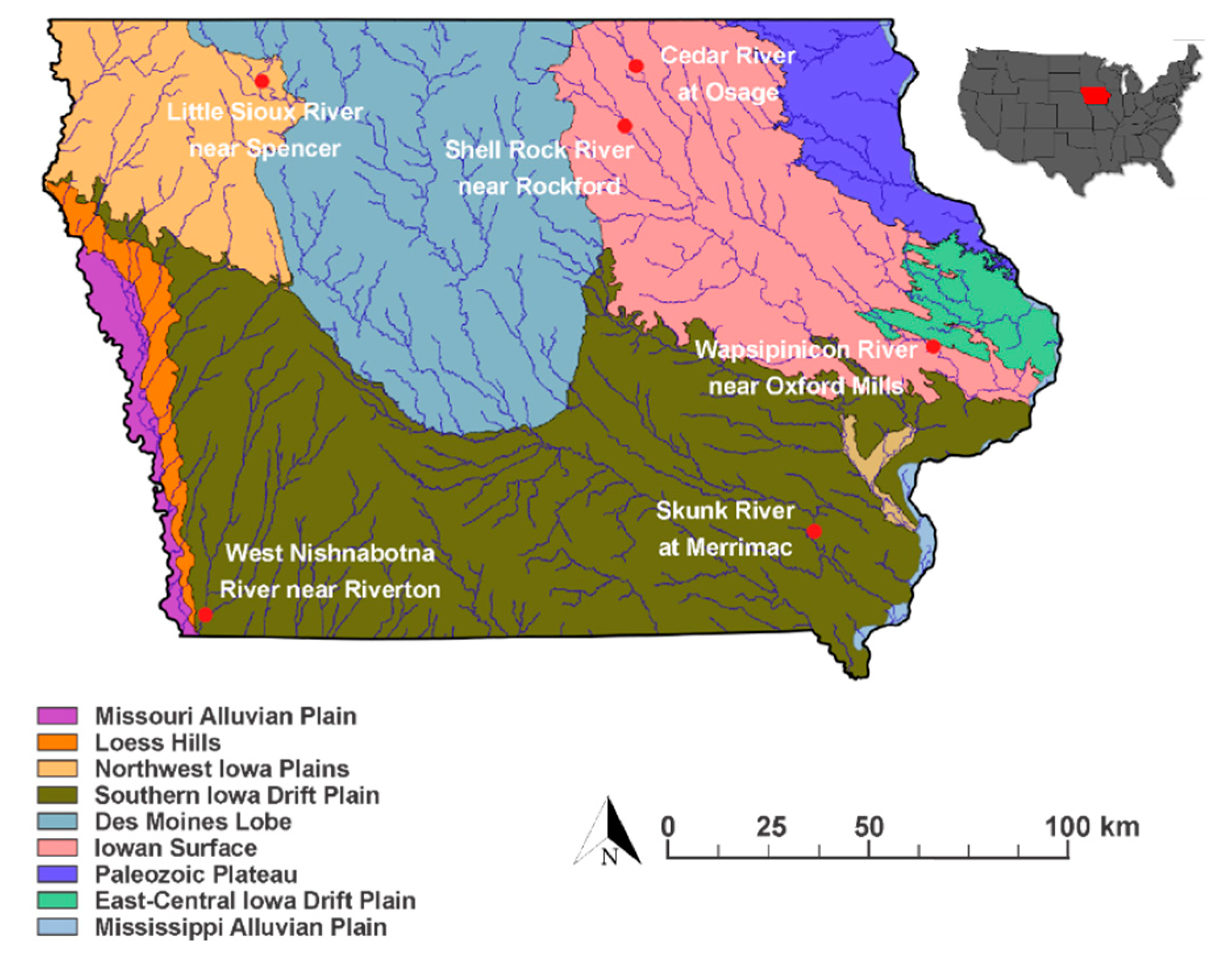
2. Study Area

The selected USGS gauging sites in Iowa are as follows: (1) Skunk River at Merrimac (05473065); (2) Wapsipinicon River at Oxford Mills (05421760); (3) Cedar River near Osage (05457505); (4) Little Sioux River near Spencer (06604440); (5) Shell Rock River near Rockford (05460400); and (6) West Nishnabotna River near Riverton (06808820). Red dots in Figure 1 show the location of the selected sites.

2.1. River Morphology

Iowa has many large rivers and hundreds of small brooks and creeks. These large and small drainageways construct distinctive, flat-floored corridors known as alluvial plains which are underlain by water-transported deposits. These topographic corridors weave throughout the state’s other landform regions, but together they constitute the Iowa’s physiographic regions, the Alluvial Plains. Figure 1 shows the landform regions of Iowa and the study sites they belong to.

During thousands of years since the various Pleistocene glaciers melted from Iowa, rivers have carved the state’s valleys and partially filled them with layered deposits of gravel, sand, silt, and clay. Along shallow stream channels, it is easy to observe individual particles of sediment being swept quickly downstream through narrow chutes. Sediment grains may lodge temporarily in a quiet pool or at the downstream end of a rippled shoal of other grains. On the other hand, more water and stronger currents can carry greater amounts of larger-diameter materials such as pebbles, cobbles, and boulders over longer distances. Lower velocities cause deposition of the coarser load and transport of only finer grained particles of silt and clay [9].

Table 1. List of USGS sites considered, available time period of rating curve and shift records, basin upstream area, soil texture and land use.

Name (USGS Code)	Period of Study	Area (km2)	Soil Texture (Bed Material)	Land Use (Flood Plain) [10]
Skunk River at Merrimac (05473065)	April 2010–January 2017	8360	silt loam	Cultivated Crops
Wapsipinicon River at Oxford Mills (05421760)	April 2010– January 2017	4628	loam	Woody Wetlands/Developed, Open Space
Cedar River at Osage (05457505)	March 2010– January 2017	2168	loam	Pasture/Hay/Deciduous Forest
Little Sioux River near Spencer (06604440)	March 2010–December 2016	1350	loam	Cultivated Crops
Shell Rock River near Rockford (05460400)	April 2010–January 2017	3230	loam	Cultivated Crops
West Nishnabotna River at Riverton (06808820)	March 2010–January 2017	4254	silt loam	Emergent Herbaceous Wetlands/Cultivated Crops

shows the bed material present at each of the studied sites.

Floodplains are submerged when a river channel carries excess water, as often occurs in the spring after snowmelt or heavy rains. In river valleys, active erosion and deposition take place on floodplains, and valley floors are often scarred with low ridges and swales marking former positions of a river channel. In the case of Iowa, in addition to urban and industrial use, valleys support intensive agriculture, expanding recreational activities, increased pumping of groundwater for urban, industrial, and irrigation uses, extraction of sand and gravel resources, and important wetland habitats, and they continue to perform their geologically designed function of accommodating floodwaters [9]. Table 1 shows the land use in the floodplain at each site.

2.2. Rating Curve Information

The USGS provided the rating curve records for these six USGS gauging sites. This information consists of the base rating curve data developed for each site during the active period and the corresponding shift values applied for each rating curve. Table 1 shows the period of information available for each gauging site.

Every rating curve for a specific gaging station should be identified with a number. The preferred numbering system should be a simple, consecutive number, with the earliest used rating as number 1, the next rating number 2, and so forth. Although not recommended, alphanumeric numbers should be permitted, as well as decimal number combinations such as 3.2 or 4.2b. Gaging stations with long periods of record may have old ratings that either are identified only by dates of use or consecutive numbers. These older ratings may no longer be in use, and in many cases may not be entered to the electronic processing system. It is recommended, however, that the old numbers be retained whenever possible, and that newer ratings that are entered to the electronic processing system be numbered in the same sequence [2] (p. 46).

Rating curves occasionally may require updating or revision. Updates usually are composed of extrapolating either the low end or the high end of the rating. If no change is made to the available part of the rating, and it is simply extrapolated (either end, or both ends), then the electronic processing system should retain the rating with no change in the rating number. However, it is possible to renumber the rating, if desired. Revisions to an existing rating, or to a segment of an existing rating, require renumbering, and revision of the period of use. In effect, a new rating is established [2] (p. 48).

3. Materials and Methods

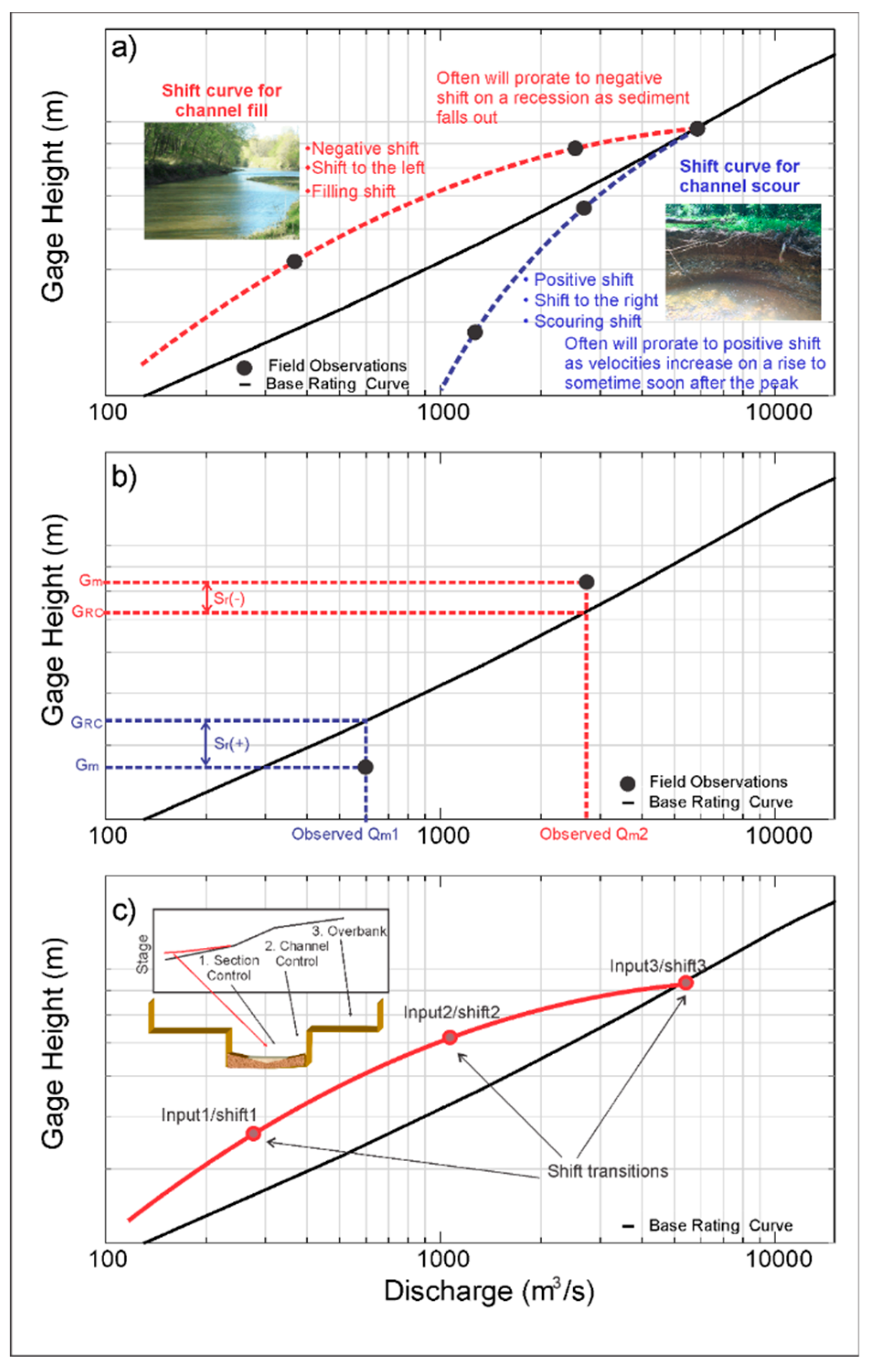
3.1. Obtaining Adjusted Rating Curves from Shifts (Shifts for Stage–Discharge Ratings)

Periodic measurements obtained by USGS allow us to decide whether an active rating curve data is still applicable. When cross-sectional geometry has changed because of channel filling/scouring, growth/removal of vegetation, or debris accumulation, it is necessary to adjust the active rating curve to match the field observations [11] (Figure 2a). In this method, a correction or shift adjustment is applied to to the base rating to reflect the temporary relation between gage height and discharge. Shifts are used until evidence of a permanent change in the rating is documented. The rating shift (S_r) associated with a measurement, is the numerical difference between the gage height (G_RC) that corresponds with the rating curve discharge for the measurement and the gage height (G_m) of the discharge measurement [2] (p. 26) (Figure 2b), and it is calculated as follows.

$$S_r=G_{RC}-G_m$$

(1)

If G_RC is smaller than G_m, the shift value will be negative, and the adjusted curve will be displaced to the left side of the base rating curve. Changes in the channel that cause negative shifts include fill or deposition in the channel, temporary dams (natural or human-made), seasonal vegetative or algal growth, and debris jams. If G_RC is greater than G_m, the shift value will be positive, and the adjusted curve will be displaced to the right side of the base rating curve. Changes in the channel that causes positive shifts include scour, gravel mining, and clearing of debris or vegetation from channel, either by floods or humans [12] (see Figure 2a).

The measurement percent difference (D_%) is the percent difference between the measured discharge (Q_m), and the rating curve discharge (Q_RC) that corresponds to the gage height of the discharge measurement, and represents the difference between the measured discharge and rating discharge if not shift is applied [2] (p. 26). The equation is

$$D_{\%}=100*(Q_m-Q_{RC})/Q_{RC}$$

(2)

If the gage height of zero flow, G₀, is determined either when a regular discharge measurement is made, or independently during a visit to the gaging station, then it is possible to compute a shift for that gage height if the rating curve is defined down to zero flow. This information can be very useful as an aid in defining the low end of a shift curve [2] (p. 26). The equation for computing the shift for the gage height of zero flow (S₀) is similar to Equation (1) for computing the rating shift, and is:

$$S_r=G_{RC}-G_O$$

(3)

The shift-adjusted rating acts as a temporary rating curve. Determining the shift transition is generally based on the geometry of the channel or controlling features of the river reach. The shape of the rating curve (plotted in log–log space) can indicate three areas: (1) section control—when a rock riffle or sandbar bed is submerged; (2) channel control—when the channel reach is controlling the flow; and (3) overbank—when the flow begins to go overbank. The shift transitions are generally at the stages when there is transition between these controlling features in the river [11]. The transition areas can change if new discharge measurements indicate something different (Figure 2c).

Figure 3 shows examples of adjusted rating curves using data from the Skunk River at Merrimac. In this section, we illustrate the methodology used to process the data from the Skunk River at Merrimac and will provide detailed analyses in the results section. The USGS established three base rating curves at this site (Figure 4a–c). A base curve remains active until measurements indicate it is necessary to incorporate significant changes to the rating curve. From Figure 4, we can see that when information on a new stage–discharge relationship becomes available, the new base rating curve is extended to include the new information (note the progression from Figure 4a to Figure 4b,c). We developed all base and shifted rating curves active over the history of the site by adjusting the base rating curves with information from shifts. Figure 3 shows rating curves (gray lines) that we found by applying shifts derived from field measurements (cyan dots) to the base rating curve (black line) active at the time.

3.2. Rating Curve Variability Analysis

We examined whether the magnitude and sign of the shift is related to the occurrence of significant streamflow events or dry periods. The shift values for each transition (section, channel, and overbank) of the control areas, were plotted on top of the discharge time series at each site (Figure 5 black, green, and blue dots). The flood level reported by the National Weather Service at each gauge is displayed in the plot to indicate when discharge values are expected to exceed the overbank limits and create a local impact. Long recession in the hydrographs denotes dry periods. During 2012, Iowa experienced a severe drought [13]; most of the hydrologic activity during that year was caused by snowmelt in the spring months. We evaluated whether variation in shift values is a function of the season (Figure 6). To achieve this, we calculated the change in consecutive shift values and found the season when it happened to determine if there is any systematic behavior. The figure also helps to identify the years with more activity in the channel. The period between 2013 and 2016 was very active, with occurrence of several high flow events.

Figure 7a shows the family of adjusted curves obtained following the methodology described above. For that dataset of curves, we estimated the number of days each curve was in operation. The rating curves with shorter durations appear in blue colors, whereas the more persistent curves are red (see Figure 7b). Channels with temporally stable geometries should ideally contain reddish colored curves. No rating is expected to be entirely stable. However, if stable geometric conditions exist in the channel, we should expect relatively low variability. We determined the median (or 50% quantile) and the range between the 25% and 75% quantiles of stage values for every discharge value in the study period (Figure 7c). To estimate quantiles consistently, it is necessary to weight each rating curve by the number of days it was active.

We determined the duration (in years) that the stage–discharge relationship was valid for each individual point on the rating curves (shown in Figure 8) to quantify variability of the rating over time. Light shades of orange indicate that the individual stage–discharge relationship was valid for a short period of time because the conditions in the channel changed, whereas dark shades of red indicate that the stage–discharge relationship remained stable for a long period of time.

We summarized the analyses for all the individual site data and compared rating stability among the gauging sites by calculating the standard deviation of the stage values for each discharge. This metric quantifies the variability of the stages around the most stable stage–discharge relationship at each site. Similar to the previous analysis, we estimated the deviation by weighing each rating curve by the number of days that the curve was active.

4. Results and Discussion

We applied the methodology described in Section 3.2 to rating data from the six USGS gauging sites.

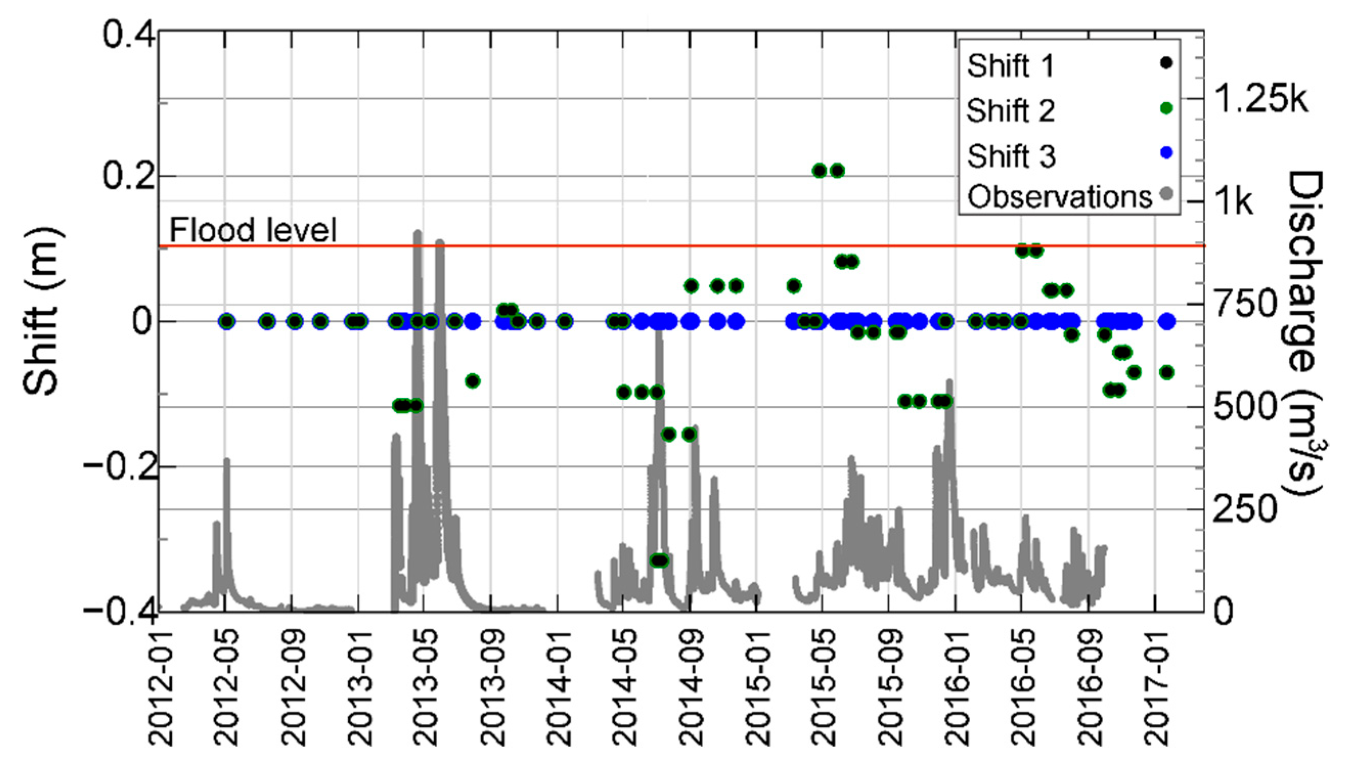
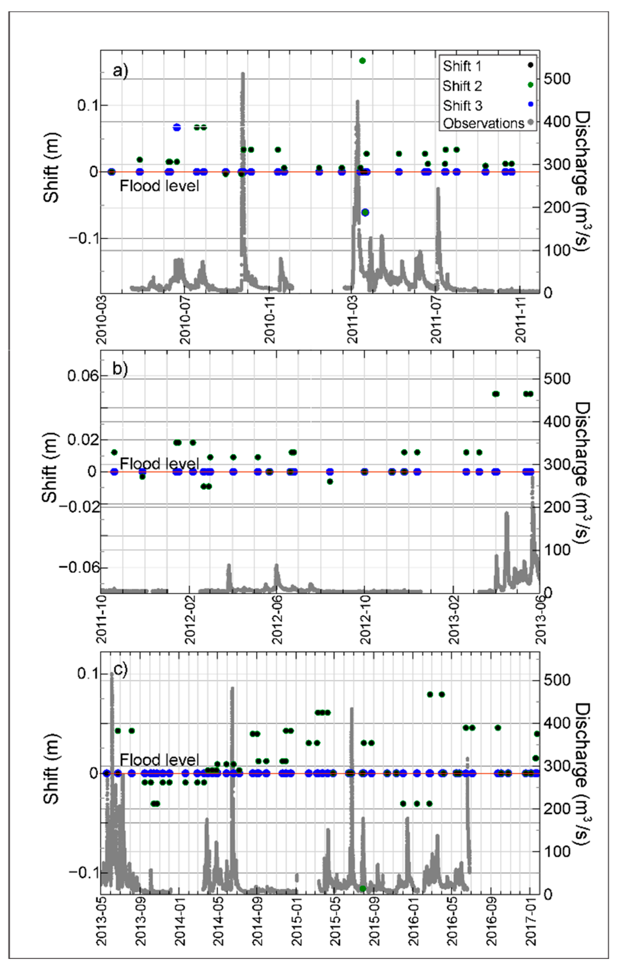
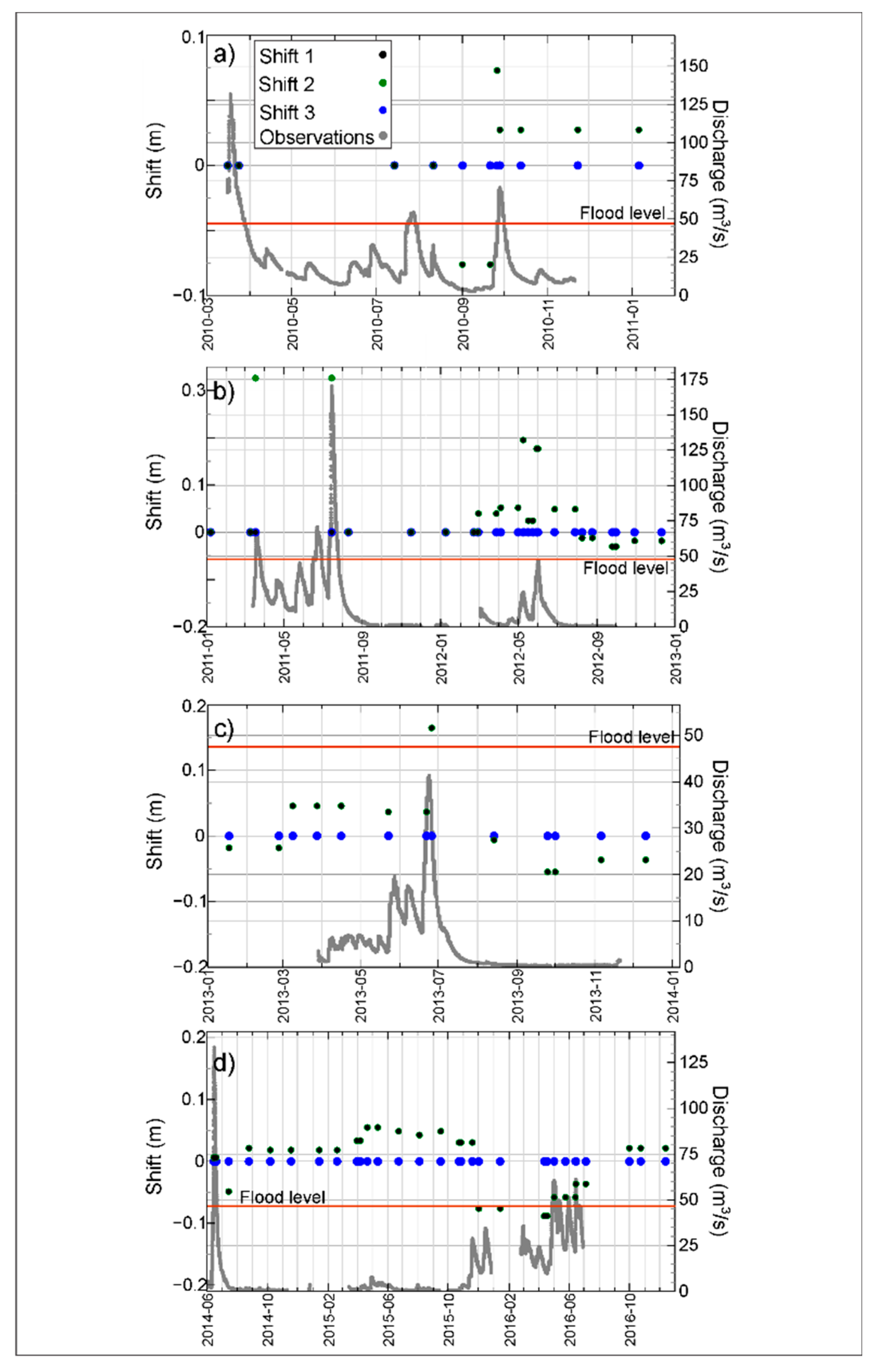
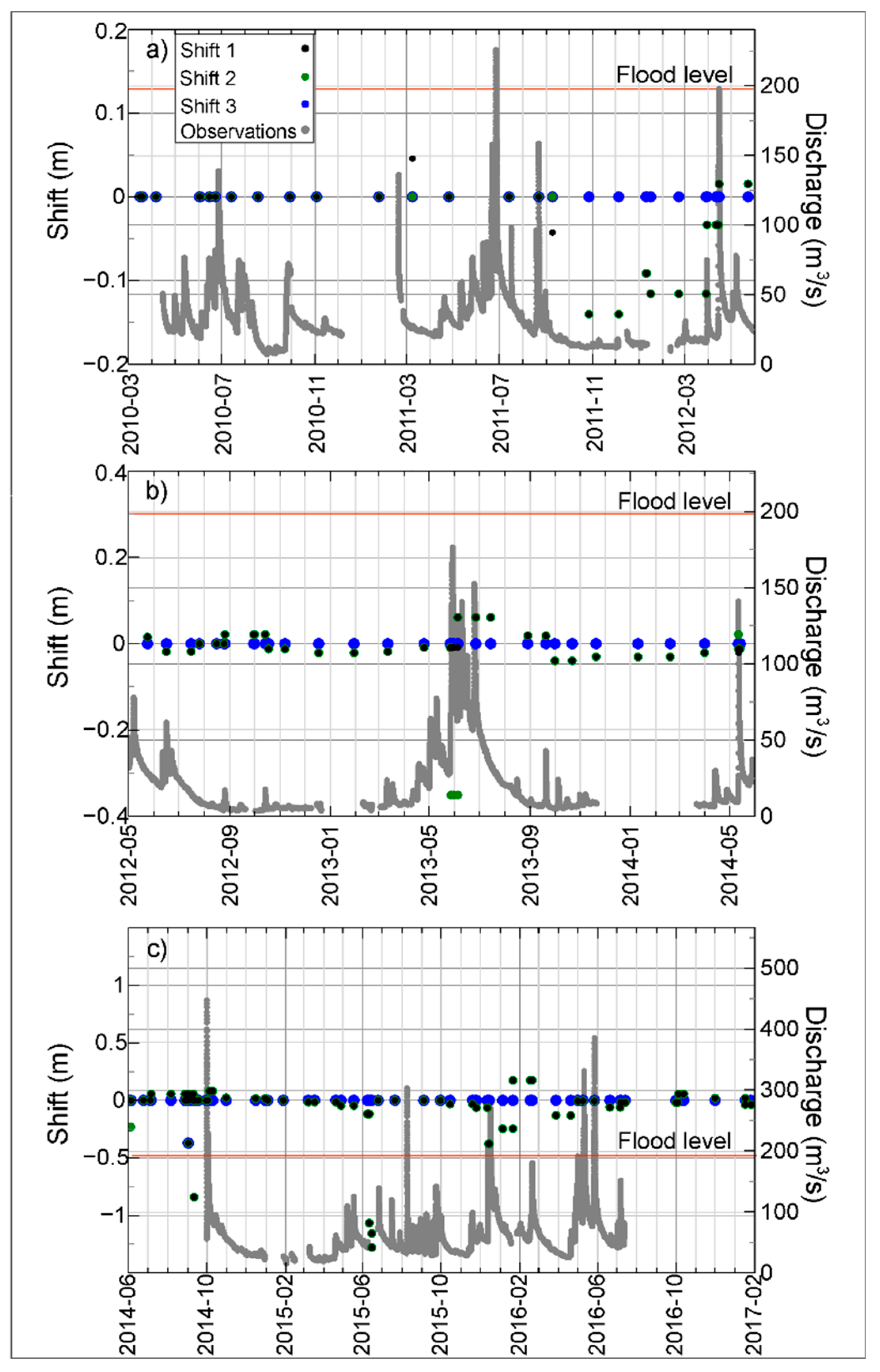
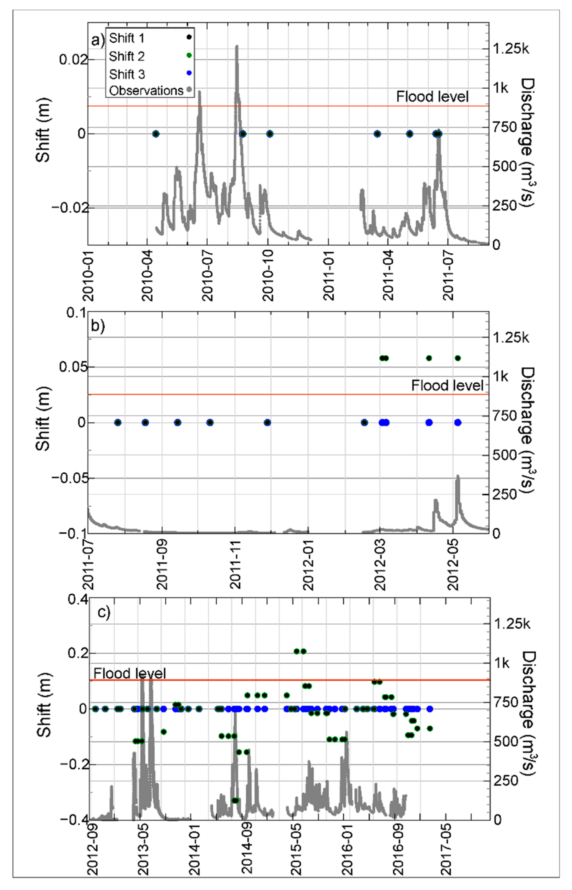
4.1. Shift Rating and Flow Events

We examined how shifts behaved for different flood event scenarios and during dry periods. We found that the sediment transport and erosion processes that take place during large streamflow events lead to changes in channel geometry that manifest as positive and negative changes in the rating shifts. We learned that during dry periods, generally minor alteration of the channel geometry occurs, this manifests as small (up to ± 0.05 m) or no change in the shift values. Figure 9 demonstrates shifting in response to flow changes for the Cedar River at Osage. After the peak flows of spring and summer of 2013 and 2016, shift for section and channel control areas generally increased. However, after peak flows in 2014 and 2015, shift values decreased, especially shift at channel control area, which during summer of 2015 fell up to −0.12 m. After the hydrograph recession, the shift decreased to zero or became negative. The shift for the overbank control area generally remains constant and zero during the entire study period, even when observations exceed the flood level, with two of exceptions: at the end of spring of 2010 when the shift rose to 0.07 m during an increase in flow, and in spring 2011 when the shift value decreases to −0.06 m after a peak flow.

As shown in Figure 10b, we observed similar behavior for the Little Sioux River near Spencer, where the shift value for the channel control area (green) reached its maximum in July 2011 after a flood event, and also in the West Nishnabotna River near Riverton (Figure 11a), where shifts at section and channel increased after the floods in spring 2012. During spring 2013, the shift at channel control area decreases significantly (up to −0.35 m) during a rapid increase in flow (Figure 11b), and then at the end of spring 2015 shifts decrease up to −1.28 m when the hydrograph falls. The shift at overbank decreases at the end of summer of 2014 but goes back to zero soon, before the peak flow in October of 2014 (Figure 11c). During the drought of 2012, most sites showed negative or zero shift values. There are also a few cases where, despite changes in flow over time, we saw no variations in the shift value. For example, Figure 12 illustrates the Skunk River at Merrimac, where shift remained at zero from 2010 to end of 2012, with some exceptions in spring 2012 when the shift for section and channel control areas had a small increase (up to 0.06 m). The shift for the overbank control area remains zero during the entire period of study, even during flood events.

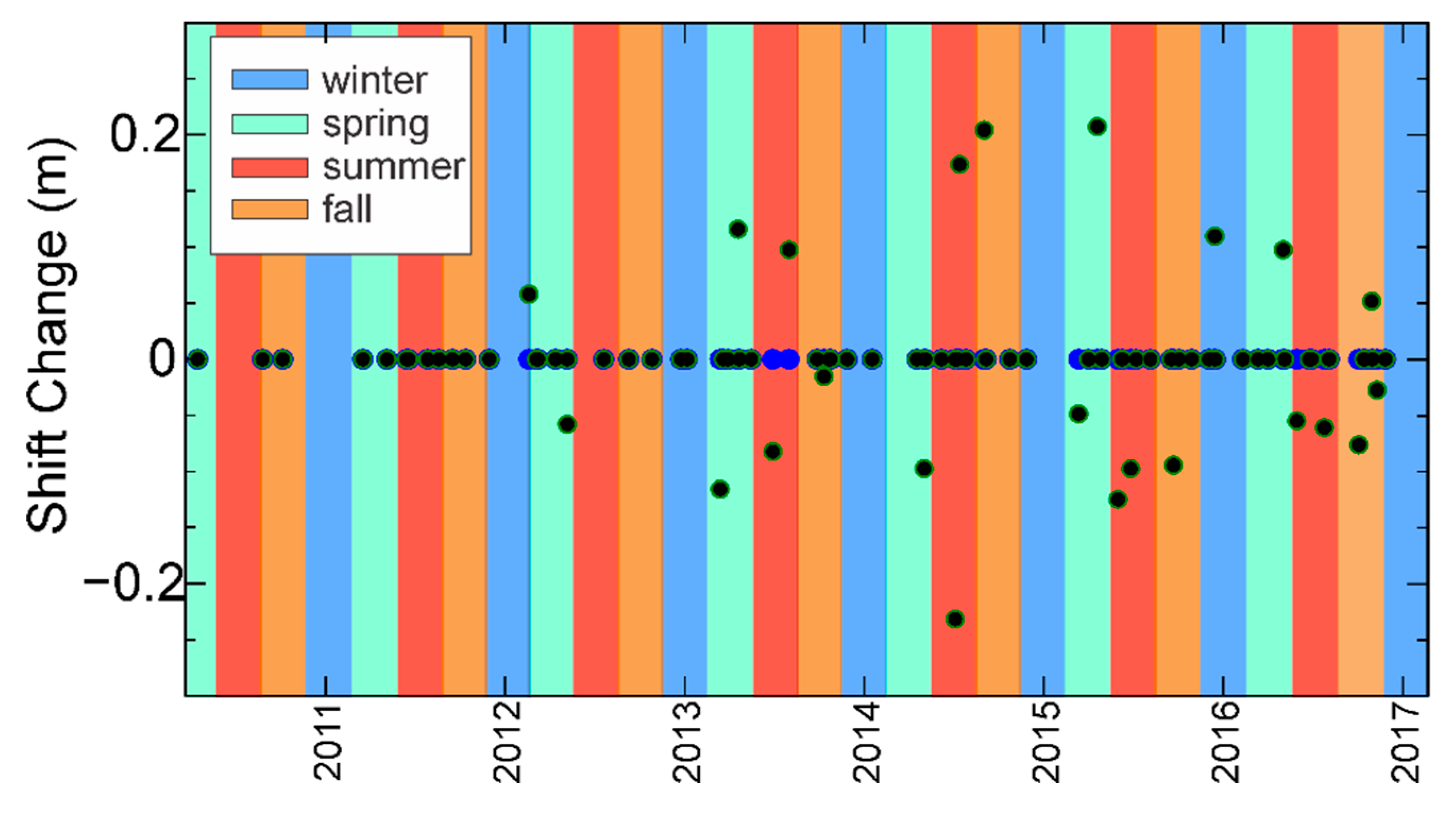
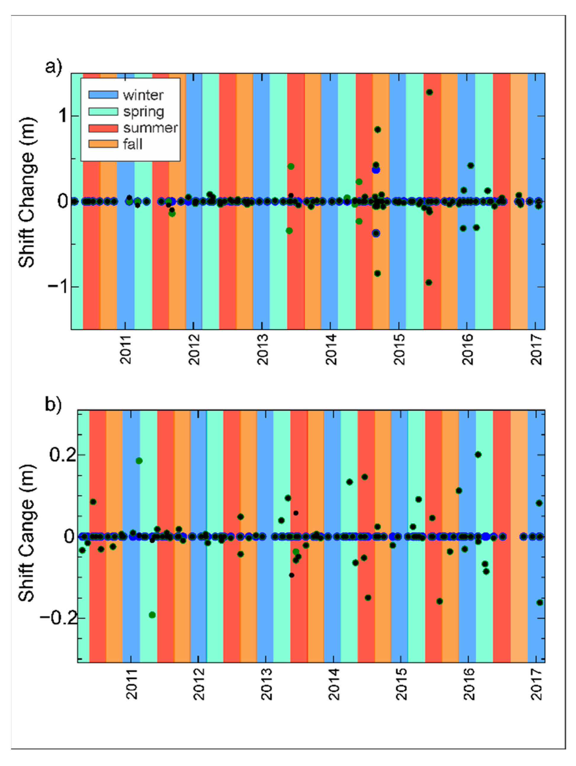
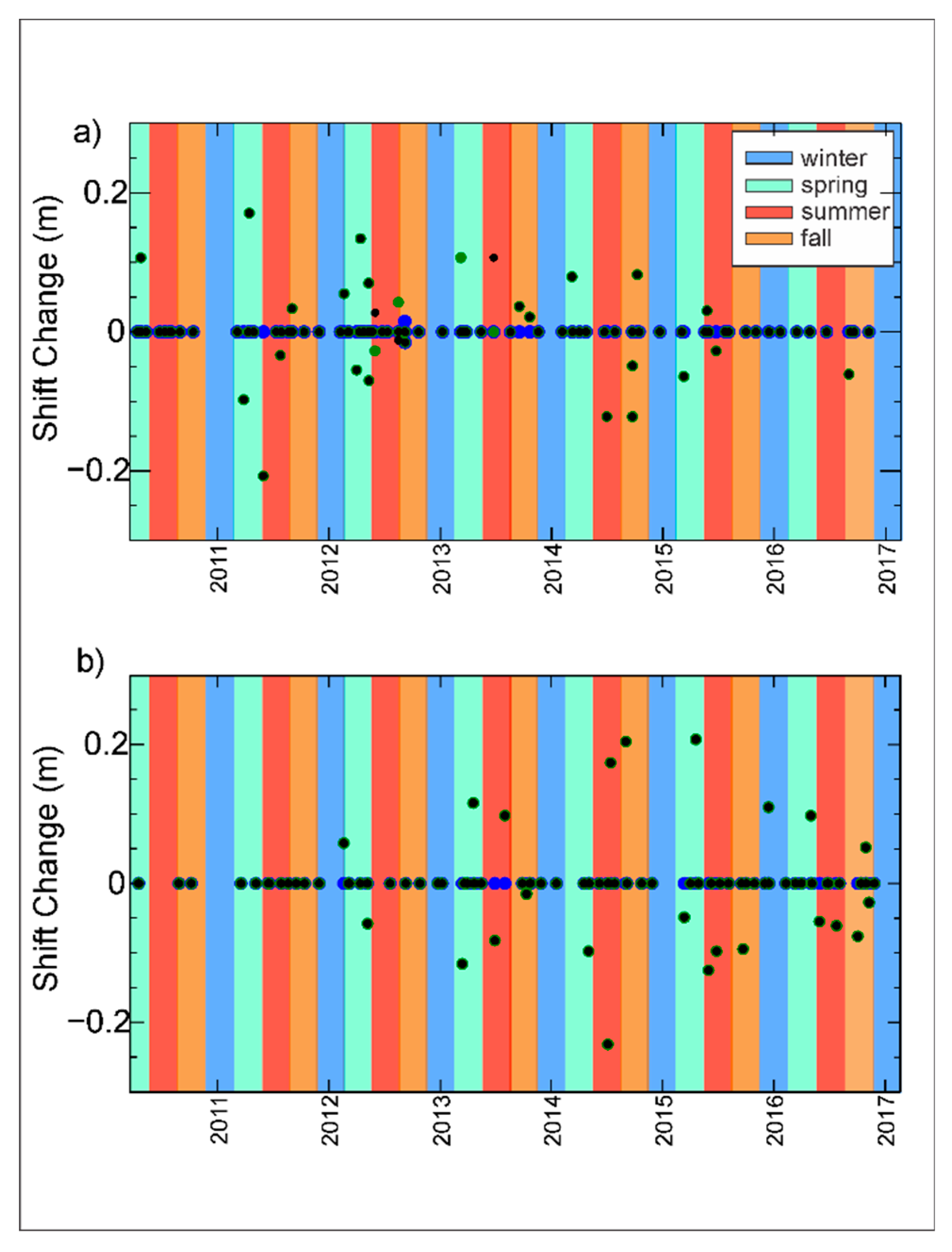
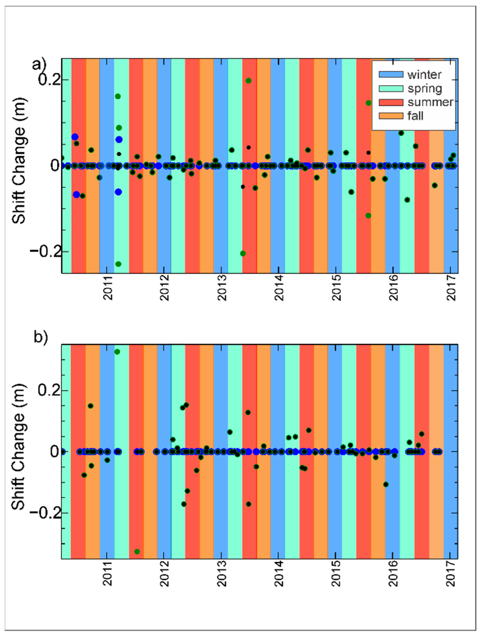
4.2. Seasonal Changes of Rating Shifts

Changes in the rating shift occur throughout all seasons, but they are more prone to happen during spring and summer. The increased rainfall and growing vegetation in the spring and summer produce changes in flow conditions and terrain roughness, which ultimately lead to changes in channel geometry. During most winter months, difficulty in obtaining measurements with ice present in the river limits rating shifts.

The gauges on the West Nishnabotna River near Riverton and the Shell Rock River at Rockford had more shift value changes. The West Nishnabotna River had 55 shift changes for section and channel control areas, mostly during spring (17 times) and summer (17 times) seasons (Figure 13a). The Shell Rock River had 53 shift changes for section and channel control areas, 17 during spring and 18 during summer. The highest shift change in the Shell Rock River occurred in February 2016, when there were no flood events or peaks (Figure 13b). Fewer shift changes occurred at the Wapsipinicon River near Oxford Mills (26 times) and the Skunk River at Merrimac (23 times). Most of the shift changes at the Wapsipinicon River near Oxford Mills occurred during spring (six increases and five decreases) (Figure 14a). For the Skunk River at Merrimac, most of the changes in the shift occurred during spring and summer. During spring, the rating shift changed eight times—four increases and four decreases. During summer, the shift value increased twice and decreased six times (Figure 14b). Most of the time, the rating shift values were zero, with some variations after peak flows registered in spring and summer. The largest decrease in the shift value was registered in summer 2014 after the peak flow on 7 July. Large increases happened in fall of 2014 and spring 2015; however, during that year, no floods events occurred. For the Cedar River at Osage, the shift value changed significantly during the four seasons; however, most of the variations occurred in spring (14 times), and summer (12 times). During spring and summer, the shift increased ten and eight times, respectively, and decreased four times in each season. During fall, the shift value showed more decreases than increases, seven and two times respectively (Figure 15a). Also, during summer of 2010 and spring of 2011, the shift for the overbank control area had some variations, but soon went back to zero after an increase in discharge. For the other sites, the shift at the overbank control area is always zero. We noted the lowest shift values in spring 2011 and the summers of 2013 and 2015 after flood events. For the Little Sioux River near Spencer, most of the shift variations occurred during spring and summer, (11 times). The highest variation of the shift at channel control area occurred in spring and summer of 2011 during flood events (Figure 15b).

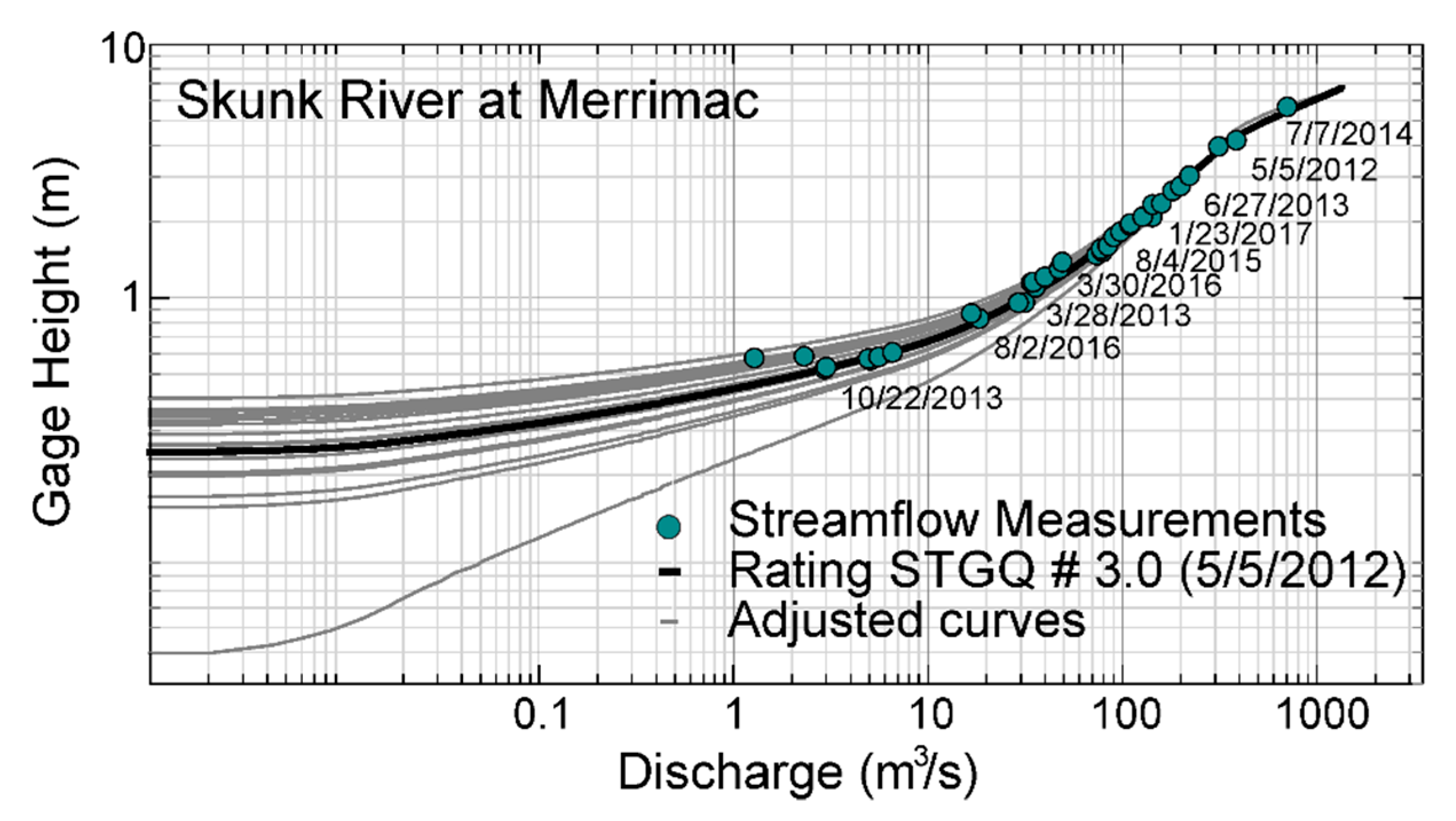
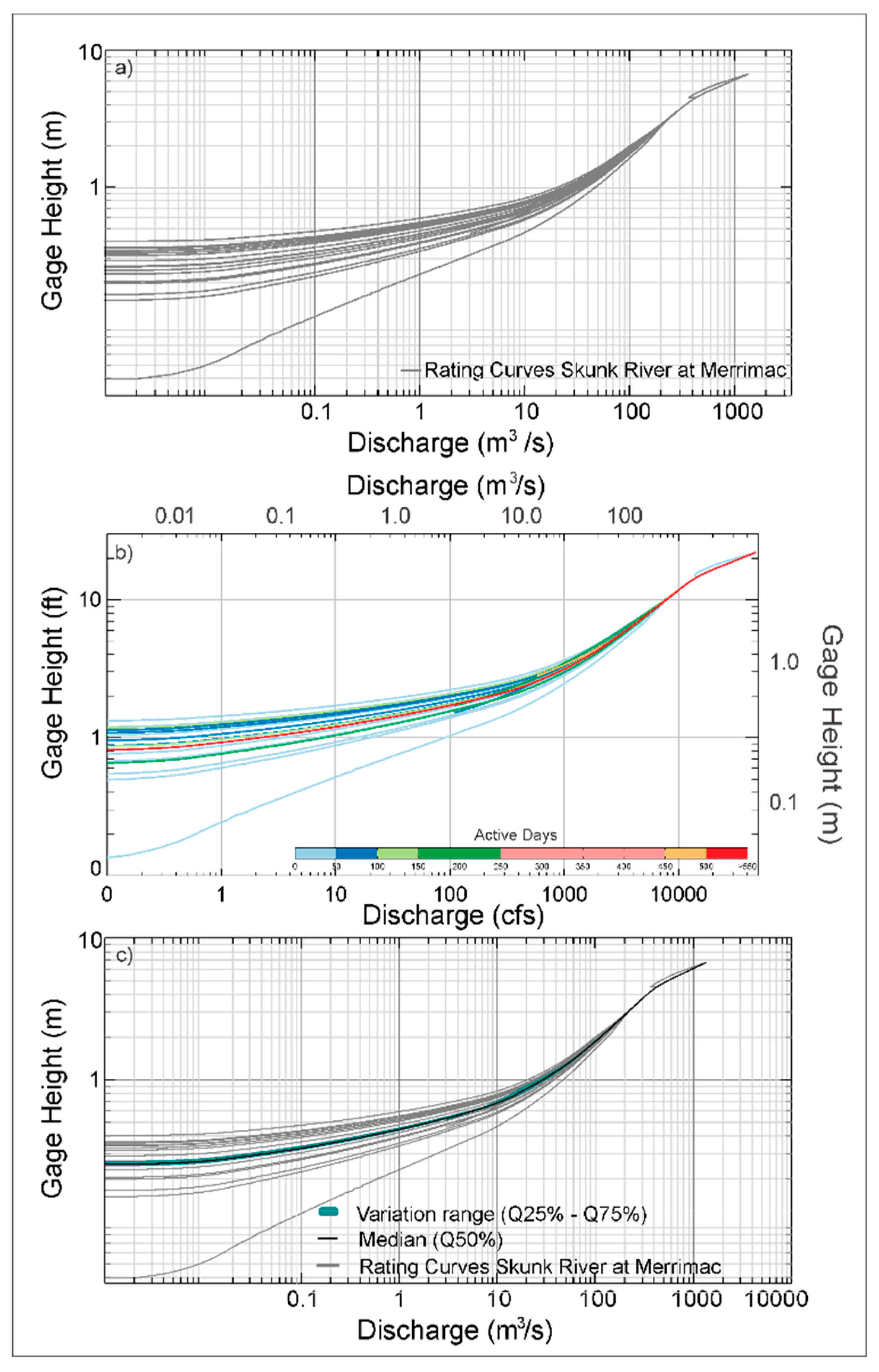
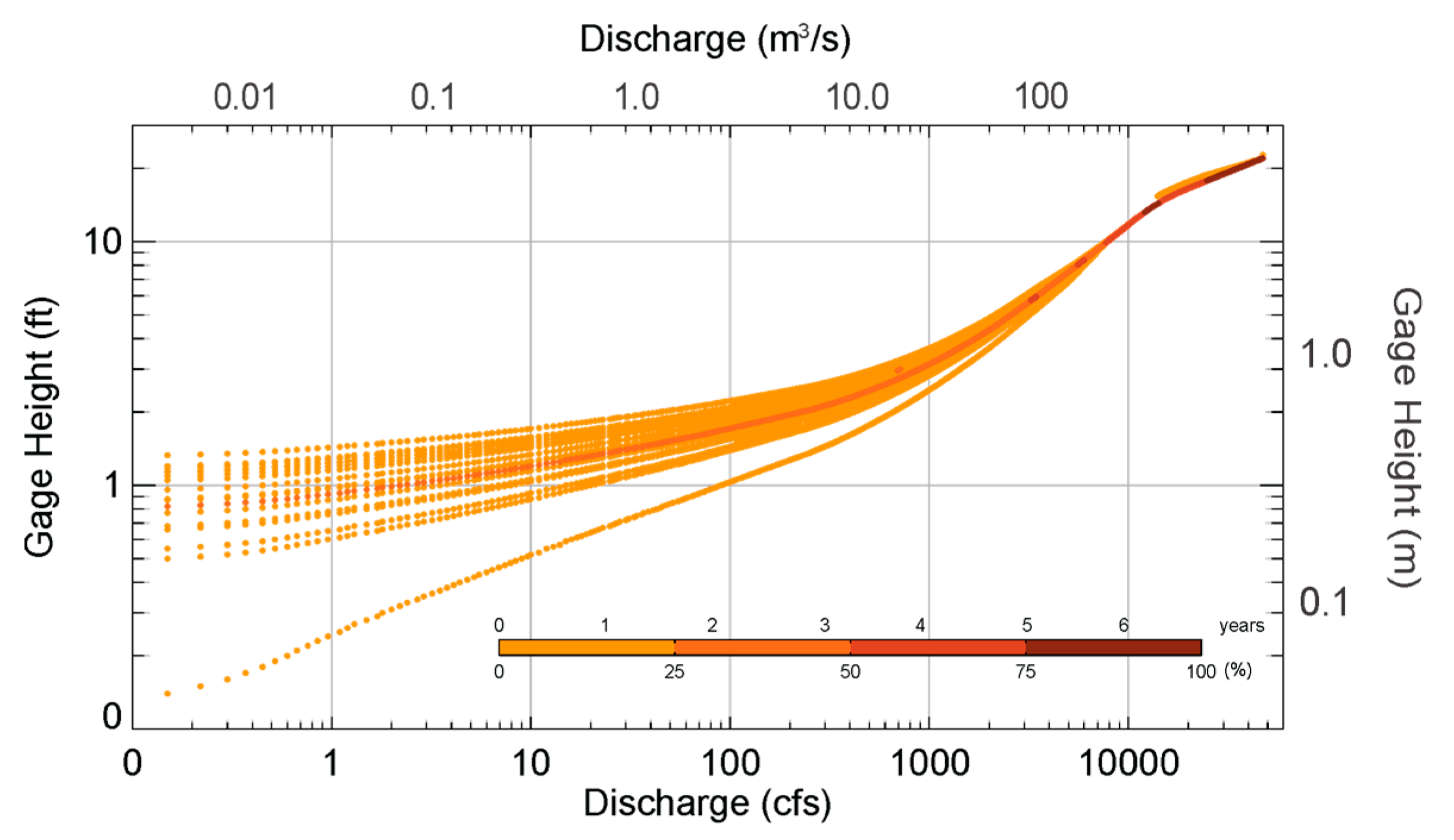
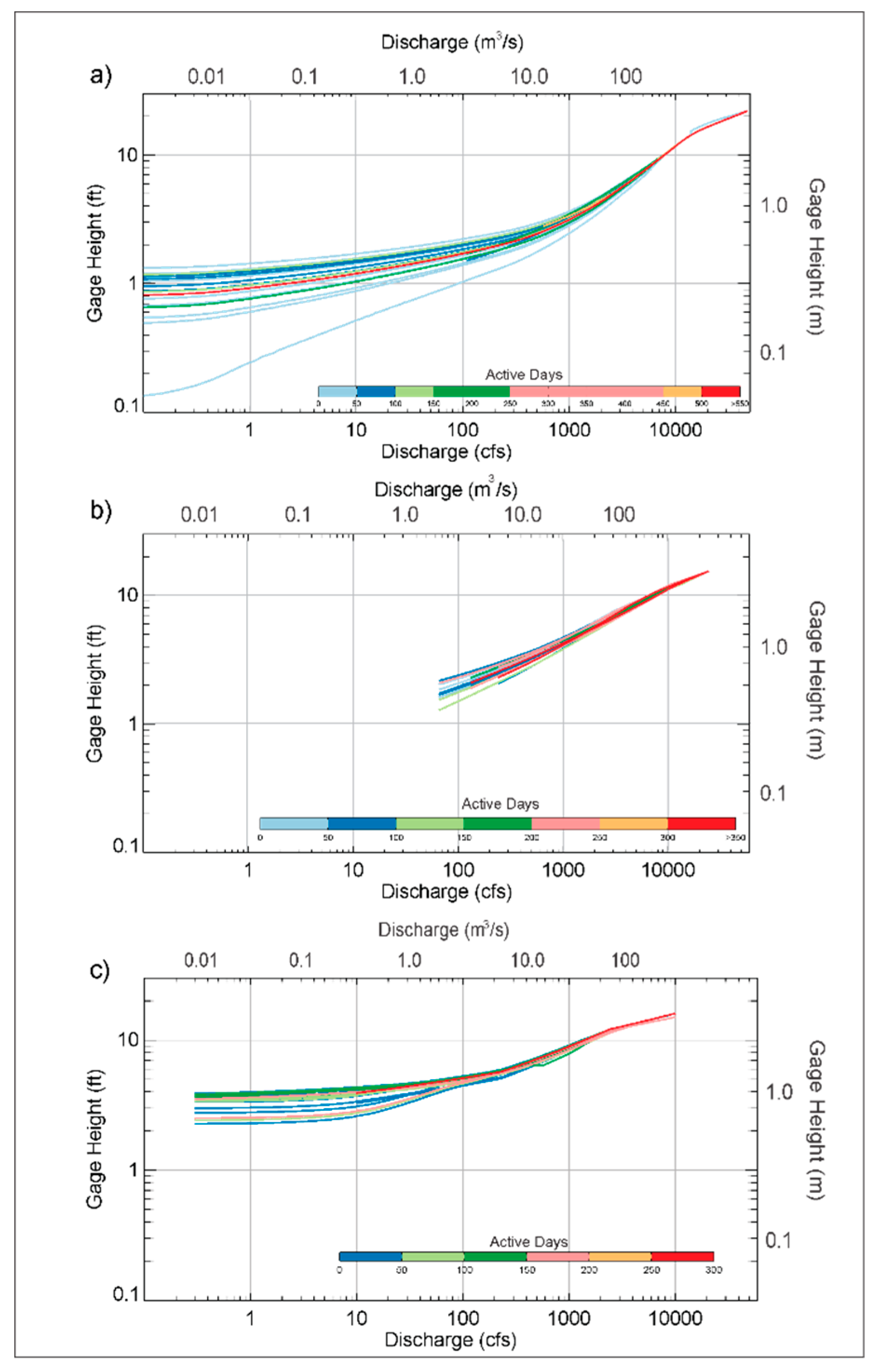
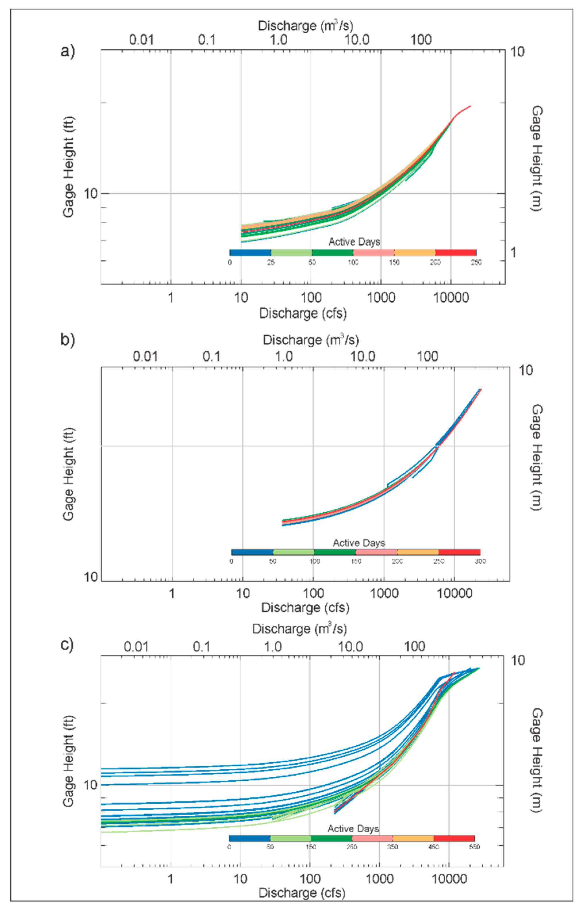
4.3. Rating Curve Variations Over Time

We calculated the number of days that each rating was active at each site. The gauge located in the Skunk River at Merrimac was active for seven years, but most of the rating curves were active for less than 100 days, reflecting low rating curve stability. Base rating curve #3.0 (Figure 16a, in red) had the longest duration with 742 days of operation. The curves for the Wapsipinicon River at Oxford Mills are shown in Figure 16b. Two of these curves had longer times of operation: base rating curve #1.0 with 367 days, and an adjustment of base rating curve #3.0 with 411 days of duration (shown in red). Figure 16c shows that most of the rating curves in the Little Sioux River near Spencer between 2010 and 2017 have short durations (under 50 days). The base rating curve #2.0 (in red) is the most stable with a duration of 273 days; however, this curve does not cover the smallest discharge values. The rating curves in the Shell Rock River near Rockford changed frequently, especially during periods of low discharge and flood events. Many curves had a duration of more than 150 days. The longest-lasting curve was an adjustment of base rating curve #3.1, with 201 active days between July 2016 and January 2017 (in red, Figure 17a), even though this time period includes one of the largest floods recorded at this site, which occurred in September 2016. In the Cedar River at Osage, the longest lasting base rating curve is #1.2 with 295 days of operation (Figure 17b). During seven years of operation for the gauge at the West Nishnabotna River near Riverton, many curves were active for short periods of time (in blue, Figure 17c), but base rating curve #1.0 did not have many changes and was active for 494 days; however this curve does not cover discharge values less than 8 m³/s.

4.4. Stage Variation and Standard Deviation

We analyzed variability in stage for a given discharge value. Also, we considered the duration of each stage–discharge relationship (Figure 18). We found that, in general, larger stage variability is observed for lower discharge values. As discharge increases, the stage has less variation, and the duration of the stage–discharge relationship is longer. However, for Cedar River at Osage (Figure 18a), we can see that even for the lower discharge values the variability in stage is smaller compared to the other sites.

Based on this idea, we explored how much stages deviate from the average, most common stage for each discharge value. We calculated the standard deviation of the stage values for each discharge (Figure 19). To make the results comparable, we normalized discharge values by the flood discharge. For most of the cases, we found higher standard deviations for small discharge values. This occurs because the river bottom is more prone to frequent changes due to sediment transport. Figure 19 shows that most of the sites exhibit greater standard stage deviation for discharge–flood ratios smaller than 1, while for larger discharge–flood ratios, the deviation decreases. We found larger deviations in the rating curve for the West Nishnabotna River (red line) where the stage deviation takes high values for the smallest discharges and for discharges between 1 and 1.7 times the flood discharge. As the flow values increase, the stage deviation tends toward zero. The Little Sioux River (orange line) also shows signs of rating curve instability; the stage deviation is relatively high for small discharges compared to the other sites, and the stage deviation does not decrease for larger discharge. Signatures of rating curve stability are visible at the Cedar River at Osage (yellow line), with constant low stage deviation through the range of discharge.

5. Conclusions

In this paper, we developed a methodology to analyze the stability of the stage–discharge relationship, based on the variability of observed rating curves at six gauges in Iowa. We implemented procedures used by USGS to obtain adjusted rating curves that were available over time for the sites of study using base rating curves and shift records. We analyzed the temporal variability of the stage–discharge relationships. We proposed an approach to quantify the variability of the stage–discharge relationship over time. Based on these results, we conclude that:

• Additional data is required to conclude about the relation between rating curve stability and the material of the stream bed. The physical characteristics of the six study sites are very similar. The material of the stream bed is basically silty loam soil and, in most of them, the land use of the floodplain for the last 10 years has been cultivation. The main differences between these sites is the drainage area. Channels with larger areas are more prone to present more changes in their geometry than channels with smaller drainage areas, especially during flow changes. This is reflected in the variations of the shift values.
• The sediment transport and erosion processes that take place during large streamflow events lead to modifications in channel geometry that manifest as positive and negative changes in the rating shifts. We also found that during dry periods, little alteration of the channel geometry generally occurs; this is manifested as small or no change in the shift values.
• Adjustments in the rating curve occur through all seasons, but they are more prone to happen during spring and summer, the seasons with more rainfall in Iowa. The increase of rainfall and growing vegetation during spring and summer produces changes in the flow conditions, changes in the roughness of terrain, and ultimately, changes to the channel geometry.
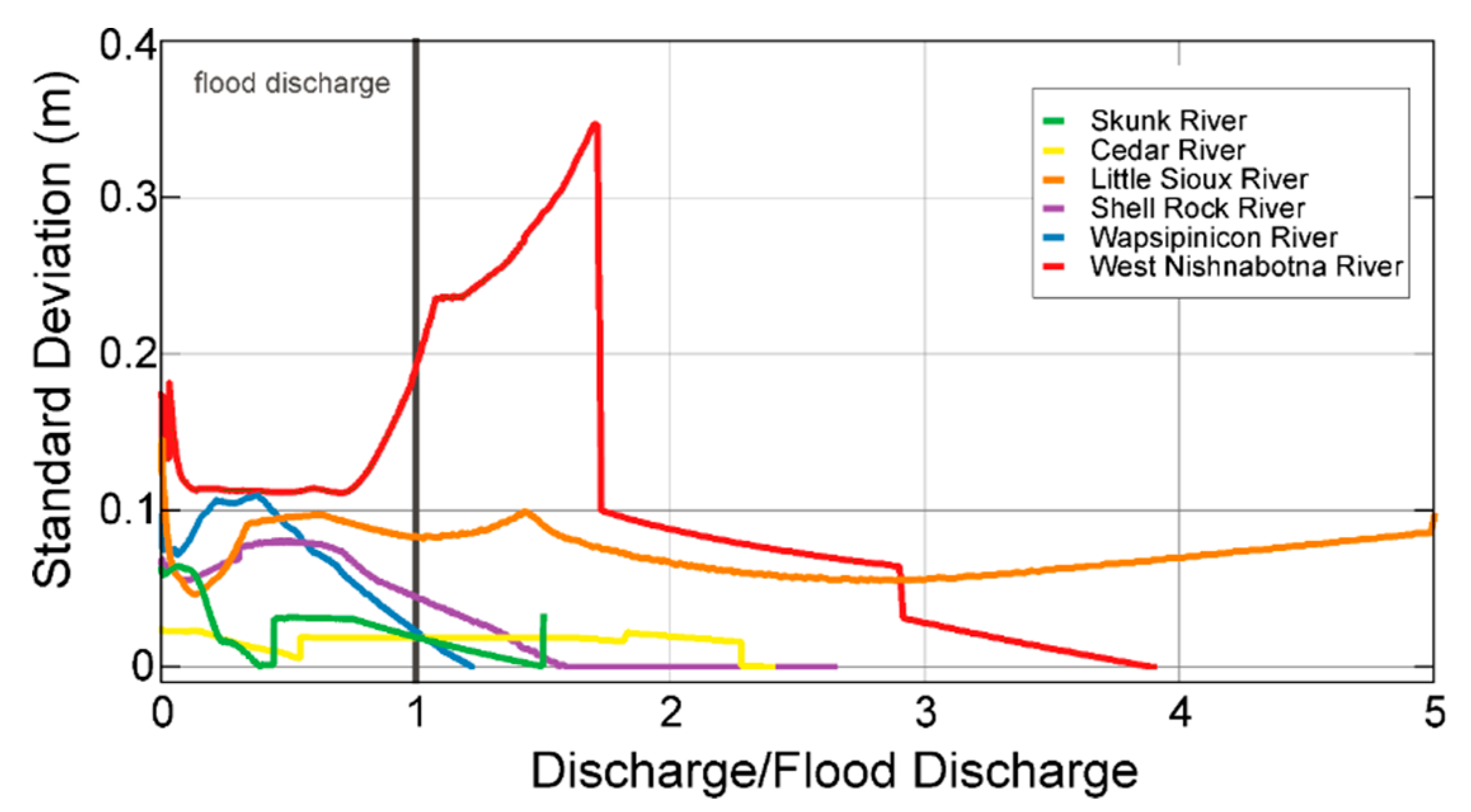
• The greater stage variability in the stage–discharge relationship is observed for lower values of discharge. As discharge increases, the stage has less variation, and the duration of the stage–discharge relation is longer. This is the consequence of the frequent variation of the shift at section and channel control areas, and less variation at the overbank control area. The proposed comparison between stage deviation and discharge–flood ratio provides elements to determine if the stage–discharge relationship at one site is stable.
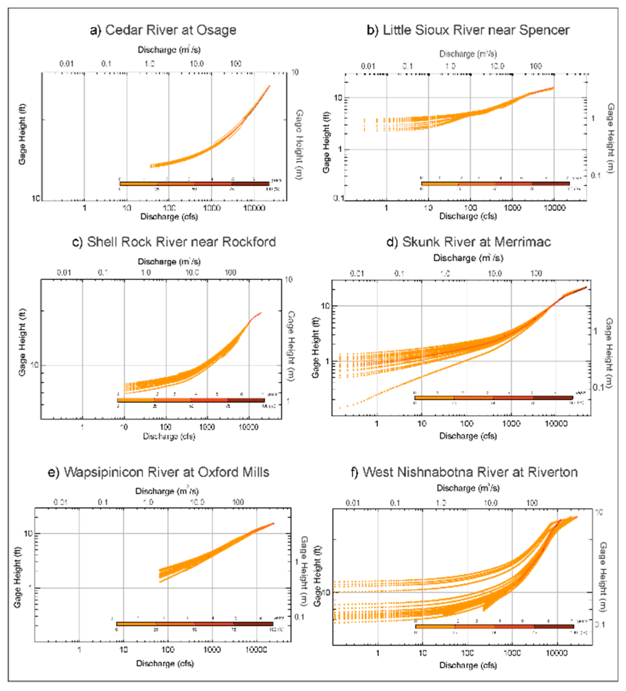
• For the 6 cases analyzed in our study, the site located in Cedar River at Osage, is the best candidate to use a synthetic rating curve instead of traditional ratings, as this site presents more stability for the entire ranges of discharge. The shift changes in Cedar River were very few and low probably because its small drainage area compared to the other study sites, which favors stability in channel geometry even during large flow events.
• A good alternative to rating curve maintenance is continuous water level monitoring coupled with use of synthetic rating curves. The Iowa Flood Center (IFC) developed and maintains a statewide network of stream stage sensors (around 250 along the state of Iowa) designed to measure stream height and transmit data automatically every 15 min to the Iowa Flood Information System (IFIS), where one can view the sensor locations and data in real time. This kind of information could help to complement the use of synthetic rating curves at a much lower cost.
• The results of the proposed methodology can support the decision to use synthetic rating curves instead of traditional ratings at streamflow gauges.

This study focuses on the analysis of rating curve data. We recommend including additional information about sediment transport modeling and geomorphologic characteristics in future studies.

References

- Herschy, R.W.; Herschy, R.W. Hydrometry: Principles and Practices, 2nd ed.; Wiley: Chichester, UK, 1999; p. 376. [Google Scholar]
- Sauer, V.B. Standards for the Analysis and Processing of Surface-Water Data and Information Using Electronic Methods. US Geol. Surv. Water Resour. Investig. 2002, 1, 106. [Google Scholar] [CrossRef]
- Fontaine, R.A.; Moss, M.; Smath, J.; Thomas, W. Cost-Effectiveness of the Stream-Gaging Program in Maine: A Prototype for Nationwide Implementation; Department of the Interior, US Geological Survey: Alexandria, VA, USA, 1984; Volume 2244. [CrossRef]
- Church, M. Channel Stability: Morphodynamics and the Morphology of Rivers. In Recent Trends in Environmental Hydraulics; Springer Science and Business Media LLC: Cham, Switzerland, 2015; pp. 281–321. [Google Scholar]
- Kennedy, E. Computation of continuous records of streamflow. Tech. Water Resour. Investig. U.S. Geol. Surv. 1983, 53. [Google Scholar] [CrossRef]
- Kennedy, E.J. Discharge Ratings at Gaging Stations; Department of the Interior, US Geological Survey: Alexandria, VA, USA, 1984; p. 58. [CrossRef]
- Fenton, J.D.; Keller, R.J. The Calculation of Streamflow from Measurements of Stage; Tech. Rep. 01/6; Cooperative Research Centre for Catchment Hydrology: Clayton, Victoria, Australia, 2001; p. 77. [Google Scholar]
- Pelletier, P.M. Uncertainties in the single determination of river discharge: A literature review. Can. J. Civ. Eng. 1988, 15, 834–850. [Google Scholar] [CrossRef]
- Prior, J.C. Landforms of Iowa; University of Iowa Press: Iowa City, IA, USA, 1991; ISBN 1587291959. [Google Scholar]
- Torbick, N.; Lusch, D.; Qi, J.; Moore, N.; Olson, J.; Ge, J. Developing land use/land cover parameterization for climate–land modelling in East Africa. Int. J. Remot. Sens. 2006, 27, 4227–4244. [Google Scholar] [CrossRef]
- Rantz, S.E. Measurement and Computation of Streamflow: Volume 2. Computation of Discharge; Department of the Interior, US Geological Survey: Washington, DC, USA, 1982; Volume 2, p. 389.
- U.S. Geological Survey. Available online: https://waterdata.usgs.gov/nwisweb/local/state/ca/text/whatisarating.html (accessed on 1 March 2019).
- Hillacker, H.J. The Drought of 2012 in Iowa Climatology Summary; Iowa Department of Agriculture and Land Stewardship: Desmoines, IA, USA, 2012; p. 6. [Google Scholar]