Abstract
In this paper, the temporal tendencies of temperature data from the island of Sardinia (Italy) were analyzed by considering 48 data series in the period 1982–2011. In particular, monthly temperatures (maximum and minimum), and some indices of daily extremes were evaluated and tested to detect trends using the Mann-Kendall non-parametric test. Results showed a positive trend in the spring months and a marked negative trend in the autumn-winter months for minimum temperatures. As regards maximum temperatures, almost all months showed positive trends, although an opposite behavior was detected in September and in the winter months. With respect to the extreme indices, a general increasing trend of the series was detected for the diurnal temperature range (DTR), frost days (FD), summer days (SU25), warm (WSDI) and cold (CSDI) spells. As regards tropical nights (TR20), an equal distribution of positive and negative trends has emerged. Results of the spatial analysis performed on the trend marks suggested that Sardinia’s topography could influence temperature variability.
1. Introduction
In its latest special report, the IPCC evidenced a temperature rise of approximately 1.0 °C above pre-industrial levels, caused by human activities, and forecast that it will likely reach 1.5 °C between 2030 and 2052 [1]. Due to global warming, over the last decades, temperature behavior has been the focus of several studies, which confirmed the mean temperature increase at different spatial scales [2,3,4,5]. Even though trend assessment of mean temperature is significant, analysis of the extreme temperature tendencies, particularly at small spatial scales is paramount, given its impacts on several natural processes and human activities, such as hydrology, food security assessment, crops, agro-ecological zoning, as well as human health and comfort [6,7]. In fact, temperature increase can affect hydrological processes, speeding up the circulation of water vapor and influencing the spatiotemporal distribution and intensity of precipitation [8]. It also directly influences hydrological features such as evaporation, runoff and soil water, which could easily raise the number of extreme climate events. Therefore, the occurrence frequency and strength of droughts and floods will increase, and the contradictory relationship between water supply and demand will become more serious [9]. Furthermore, when high temperature values rise above critical levels, a rise in human death rates can be observed [10]. For example, a severe heat wave affected Europe during the summer of 2003, with considerable health, ecological, societal, and economic impacts [11]. Among these, a high death rate among the elderly, documented in several countries was undoubtedly the most significant [12]. The ecological impacts involved wildfires, increased contamination, a decrease in livestock, low quality crops, and a reduction of forest areas, flora and fauna [13,14,15,16]. The economic damages in 2003 have been evaluated to be more than 10 billion of US dollars [11]. Several climate extreme indices have been proposed and some global high-spatial-resolution climate extreme indices datasets, derived from quality-controlled historical observations or reanalysis data products, have been created in order to support scientists in regional and global temperature extremes analyses, and also to aid climate modelers and policymakers in the assessment of sectoral impacts [17,18]. In fact, for the scientific community working on climate change impacts and variability, the use of extreme indicators allows a better understanding of the role of extreme events and sectoral implications. In this context, temperature extremes have been largely studied at the regional scale, such as in western and central Europe [19,20], northern Europe [21], North America [22], South America [23,24], China [25,26], New Zealand [27], India [28,29,30], northwestern Africa [31,32] and the Arabian peninsula [33]. Additionally, in the Mediterranean area, which is considered sensitive to global warming [34], temperature extremes have been widely investigated by the climate research community. For example, Hertig et al. [35] and Efthymiadis et al. [36], by analyzing the trends of temperature extremes, identified a different spatial pattern with warming and cooling tendencies involving the western and the eastern side of Mediterranean, respectively. In particular, this trend seemed more marked in winter and more homogeneous in summer, due to an increase/decrease in the warm/cold extremes across the Mediterranean basin. Although in Italy several authors detected a general increase in temperatures over the last decades [37,38,39,40,41,42,43], only a few studies have focused on temperature extremes and their temporal evolution. In particular, Toreti and Desiato [44] analyzed the trend behavior of minimum and maximum daily temperatures in the period 1961–2004, while Simolo et al. [45] studied the Italian daily temperature anomalies by detecting the variations in their probability density functions. At a regional scale, in northern Italy, extreme temperature changes have been analyzed in the northwestern Italian Alps [46] and in Emilia Romagna [47]. In central Italy, daily temperature extremes have been investigated in Marche and Abruzzo, the central Adriatic regions of Italy, in the period 1980–2012 [48] and for the period 1955–2007 across Tuscany [49]. Finally, extreme temperature events (both maximum and minimum) have been studied in southern Italy by Piccarreta et al. [50] and Caloiero et al. [51], by means of several climate indices, in the Basilicata and in the Calabria regions, respectively. These studies are mainly based on trend detection by means of parametric or non-parametric tests. Parametric testing procedures are widely used in classical statistics. In parametric testing, it is necessary to assume an underlying distribution for the data (often the normal distribution), and to make assumptions that data observations are independent of one another. In non-parametric and distribution-free methods, fewer assumptions about the data are required. An assumed distribution is not necessary with such methods. However, many of these methods still rely on assumptions of independence. Generally, non-parametric tests are better suited to deal with non-normally distributed hydrometeorology data than parametric methods. The Mann-Kendall [52,53] and Spearman’s rho tests are among the most widely used trend detection tests.
In this context, the aims of the present study are: (i) to detect the temperature trends of monthly values in the Sardinia region, and (ii) to analyze the behaviors of the daily extreme temperatures in the same region, by means of 14 well-known temperature indices. This study can be considered the first effort to deal with extreme temperatures and their temporal tendencies in Sardinia, an island located in the western Mediterranean Sea, and one particularly affected by climate change. This paper is organized as follows. Section 2 describes the study area, from a geographical and climatological point of view, and the temperature database. Section 3 introduces the indices and the trend test used in this paper. Section 4 describes the results of the trend analysis performed on the monthly minimum (Section 4.1) and maximum (Section 4.2) temperature series and on the extreme temperature indices (Section 4.3). Section 5 highlights the added value of his work compared to other similar studies in different areas of the world. Finally, Section 6 presents the conclusions.
2. Study Area and Data
The Sardinia region is an island located at the center of the western Mediterranean basin (between 38°51′ N to 41°15′ N and 8°8′ E to 9°50′ E). The area of the region is more than 24,000 km2, and thus it follows Sicily (about 26,000 km2) and precedes Cyprus (10,000 km2) in the list of the largest islands in the Mediterranean Sea. The orography of the island is mainly characterized by plains, especially in the northwestern and in the southern areas, but also by alluvial valleys and mountains [54], with an average and a maximum altitude of 337 m a.s.l. and 1834 m a.s.l., respectively (Figure 1). Due to its position, the Köppen-Geiger classification [55] identifies the climate of the island as a hot-summer Mediterranean climate, thus presenting relatively mild winters (with rain) and very hot summers (often very dry).
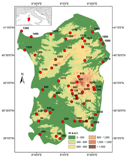
Figure 1.
Location of the selected 48 stations on a study-area digital elevation model.
In the present study, complete or near-complete records of daily temperature data have been downloaded from the website of the Sardinia Region (http://www.regione.sardegna.it) for the period 1922–2011 [56]. The database consists of high-quality rainfall and temperature data which have been extensively used in past climatological studies performed on the region, e.g., [57,58,59]. In particular, daily temperature data collected at 191 stations are available online for the period 1982–2011, with an average density of one station per 125 km2. These data have been collected following the same methodology across the different stations, and the temperature values used in the paper are the absolute maximum and minimum values registered in a day from automatic stations. In order to perform a reliable statistical analysis in this work, temperature series with more than 10% of missing data were discarded. Thus, the analyses have been performed on 48 temperature series (Figure 1), with an average density of one station per 490 km2. Table 1; Table 2 show the main statistics of the minimum and maximum temperature series, respectively.

Table 1.
Main statistics of the minimum temperature series.
Table 2.
Main statistics of the maximum temperature series.
3. Methodology
The aim of this study is to analyze the temporal characteristics of extreme temperatures in Sardinia. To achieve this, a set of well-known indices, summarizing frequency, intensity and persistence of daily temperatures were extracted from the list proposed by the Expert Team of the World Meteorological Organization and Climate Variability and Predictability (ETCCDMI), e.g., [60,61]. In particular, 14 indices have been selected (Table 3) representing the annual daily maximum and minimum temperatures extremes (TXx, TNx, TXn, TNn, all abbreviations defined in Table 3), their mean difference (DTR), the annual number of days in which temperatures exceeded a fixed threshold (FD, TR20, SU25) or percentiles (TN10p, TX10p, TN90p, TX90p, WSDI, CSDI). As a result, these indices can be grouped into three categories: warm, cold and variability indices [62]. Specifically, due to the different sampled temperature distribution, which can be detected over large areas by using indices based on fixed thresholds, the percentile thresholds-based indices are particularly important and can be considered more appropriate than the former for a spatial comparison of the extremes [63]. For example, at mid-latitude climates, a useful indicator for cases of extreme cold could be the number of days evidencing minimum temperature below 0 °C (FD) which, at extreme latitudes, represents normality during winter nights. Additionally, in mild climate settings, where the average summer maxima are around 18 °C, the number of summer days above 25 °C (SU25) could be a useful index to indicate abnormally warm conditions.
Table 3.
Extreme temperature indices recommended by the Expert Team on Climate Change Detection and Indices (ETCCDI) used in this paper.
In order to detect the existence of temporal tendencies in the monthly temperatures and in the temperature extremes, the non-parametric test of Mann-Kendall (MK) [52,53] was applied considering the statistical significance of the trend at the 90%, 95% and 99% confidence intervals.
For a series with dimension n, the MK statistic is obtained as:
in which xi and xj are the values of the variable at times i and j, respectively, with i < j.
In particular, if the xi values are independent and randomly ordered, and for a dimension n > 10, the statistic S can be represented by a normal distribution presenting zero mean and variance given by:
with ti ties number with dimension i.
Finally, the test statistic ZMK is standardized as:
Using a two-tailed test for a specified significance level α, the null hypothesis is accepted if |ZMK| is lower than Z1-α/2, otherwise the null hypothesis is rejected and the trend can be considered significant.
4. Results
4.1. Analysis of the Monthly Minimum Temperature
Figure 2 presents a summary of the trend analysis performed on the 48 monthly minimum temperature series. A prevalent positive trend has been observed in April, May and June. Specifically, in April, 58.3%, 39.6% and 20.8% of the series showed a positive trend with a significance level (SL) of 90%, 95% and 99% respectively. On the contrary, a negative trend has been detected only in 4.2% (SL = 90%) and 2.1% (SL = 95%) of the series. No significant negative trends have been identified for an SL = 99%. In May, positive (negative) trends have been detected for 40.4% (8.5%), 34.0% (2.1%) and 14.9% (no trend) of the series with a significance level (SL) of 90%, 95% and 99% respectively. In June, the percentage of series showing a positive trend is similar to the one identified in May (41.7%, 33.3% and 14.6% for the ascending SL) while a negative trend has been detected in 12.5% (SL = 90%), 8.3% (SL = 95%) and 2.1% (SL = 90%) of the series.
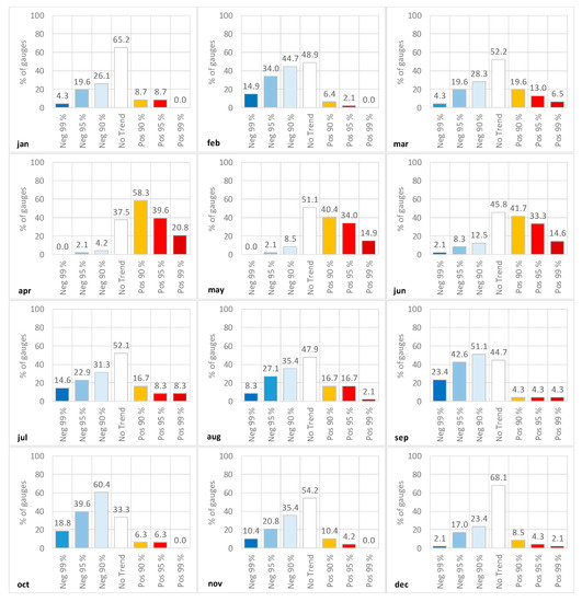
Figure 2.
Percentages of minimum temperature series presenting positive or negative trend.
The spatial distribution of the trends (SL = 95%) shows that in April, May and June the temperature series presenting increasing values are distributed across the region, while the negative trends are observed in the southern stations, especially in June, and in the eastern mountain of the region (Figure 3).
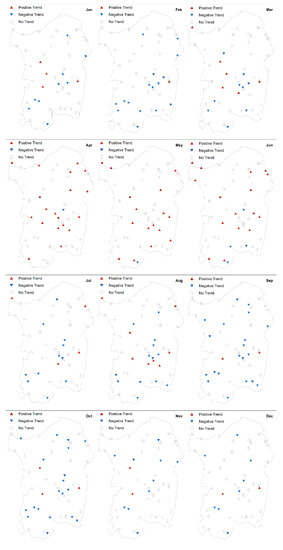
Figure 3.
Spatial distribution of the monthly minimum temperature trend.
An opposite trend behavior than in April, May and June has been detected in the other months, and in particular in the autumn–winter period (Figure 2). In fact, in February, in October and particularly in September, a marked negative trend has been identified respectively in 34.0%, 39.6% and 42.6% of the series, with a significance level of 95%, and respectively in 14.9%, 18.8% and 23.4% of the series, with a significance level of 99%. In the same months a positive trend has been detected for an SL = 90% only in 6.4%, 6.3% and 4.3% of the gauges. From the spatial analysis, the results obtained in these months (SL = 95%) evidenced a positive trend distributed across the region and in particular in the south-eastern side of the island, and scattered negative trend in the central area (Figure 3). In addition to autumn and winter, a negative trend, albeit less marked, has also been detected in March, July and August. In effect, in these months, there are few differences among the percentage of series showing a positive or a negative trend (Figure 2). In particular, in March the percentage of series showing a negative trend with an SL = 90% (28.3%) and an SL = 95% (19.6%) is slightly higher than the one presenting a positive trend, equal to 19.0% and 13.0%, respectively. On the contrary, for an SL = 99%, a higher percentage of positive trend series has been detected, 6.5% against 4.3% of negative trend series. The spatial distribution of the trend (SL = 95%) in these months did not show any peculiarity, although the positive trend seems to be mainly localized in the central area of the region (Figure 3).
4.2. Analysis of the Monthly Maximum Temperature
As regards maximum temperatures, a marked positive trend has been identified for all the monthly values, with the exception of January, September, December and, partially, October (Figure 4).
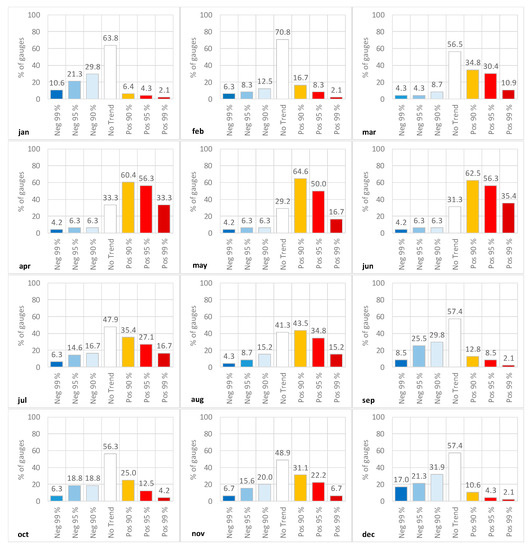
Figure 4.
Percentages of maximum temperature series presenting positive or negative trends.
The highest numbers of stations with positive trends have been identified in the spring and summer months (from March to August), with a maximum percentage in June. During this month 62.5% 56.3% and 35.4% of the stations evidenced this tendency with an SL = 90%, 95% and 99%, respectively, and a negative trend has been detected in 6.3% (SL = 90%), 6.3% (SL = 95%) and 4.2% (SL = 90%) of the series. Relevant positive trends have also been detected in April and May, when significant trends have been identified respectively in 56.3%, and 50.0% of the series, with a significance level of 95%, and respectively in 33.3% and 16.7% of the series, with a significance level of 99%. In the same months, only in 6.3% of the gauges has a positive trend has been detected for a SL = 90% (Figure 4). The spatial distribution of the trend (SL = 95%) in these months is similar to the one obtained for the minimum temperature. In fact, the temperature series presenting increasing values are distributed across the region, while the negative trends are observed around the eastern mountains of the region (Figure 5). In February, October and November, there are few differences among the percentage of series showing positive or negative trends, although the positive trend prevails, especially for lower SLs (Figure 4). In fact, the percentage of series showing a negative trend with a SL = 99% in February (6.3%), October (6.3%) and November (6.7%) is equal or slightly higher than the one presenting a positive trend, equal to 2.1%, 4.2% and 6.7%, respectively. From the spatial analysis, the results obtained in these months (SL = 95%) evidenced a positive trend distributed in the southern side of the region, and scattered negative trends in the central area (Figure 5). Finally, in January, September and December a prevailing negative trend has been identified respectively in 21.3%, 25.5% and 21.3% of the series, with a significance level of 95%, and in 10.6%, 8.5% and 17.0% of the series respectively, with a significance level of 99%. In the same months, only in 6.4%, 12.8% and 10.6% of the gauges a positive trend has been detected for an SL = 90% (Figure 4). The spatial analysis of the results obtained in these months (SL = 95%) evidenced relevant results only in January and December, with the positive trend affecting the eastern side of the island (Figure 5).
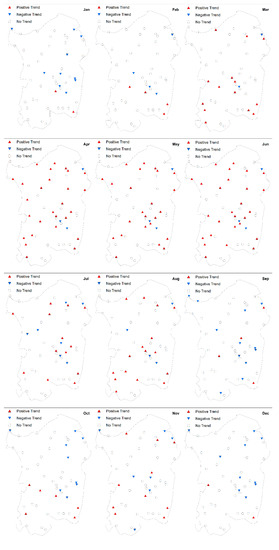
Figure 5.
Spatial distribution of monthly maximum temperature trend.
4.3. Analysis of the Extreme Temperature Indices
Given the minimum and the maximum daily temperature values recorded in Sardinia in the period 1922–2011, some extreme temperature indices have been analyzed for trend detection. With respect to TXx and TNx, which are the maximum extreme values of daily temperature, more than 50% of the series evidenced significant trends (SL = 90%). In fact, considering the TXx index, 41.7% (20.8%), 31.3% (12.5%) and 12.5% (8.3%) of the gauges evidenced a positive (negative) trend, with an SL = 90%, 95% and 99%, respectively (Figure 6).
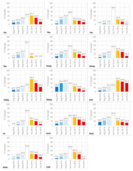
Figure 6.
Percentages of extreme temperature indices series presenting positive or negative significant trends.
An opposite trend behavior has been observed for TNx with 31.9% (SL = 90%), 23.4% (SL = 95%) and 4.3% (SL = 99%) of the series presenting a negative trend, and 19.1%, 17.0% and 10.6% of the series evidencing a positive trend for an SL equal to 90%, 95% and 99%, respectively (Figure 6). Spatially, the temperature series of TXx and TNx presenting increasing values are distributed across the region, while the negative trends are mainly concentrated around the eastern mountains and in the north-eastern side of the region (Figure 7). As regards the annual extremes minimum temperatures (TXn and TNn), an opposite trend behavior has been detected, with the temperature series showing a prevailing positive trend of TXn and a negative trend of TNn, although for both TXn and TNn the majority of the series, 70.2% and 66.7%, respectively, showed an absence of trend. In particular, for TXn, 23.4%, 12.8% and 2.1% of the series showed a positive trend with SLs of 90%, 95% and 99%, respectively. On the contrary, a negative trend has been detected only in 6.4% (SL = 90% and SL = 95%) of the series (Figure 6). For TNn 22.9% (SL = 90%), 16.7% (SL = 95%) and 2.1% (SL = 99%) of the series showed a negative trend and only 10.4% showed a positive trend for an SL = 90% (Figure 6). The spatial analysis of the trend results, for an SL = 95%, evidenced that for both TXn and TNn the significant trends are localized in the southern part of the region (Figure 7). The trend analysis performed on the extreme percentile-based indices (TN10p, TN90p, TX10p and TX90p) evidenced prevailing positive trends for TX10p, TN10p and TX90p (Figure 6). In fact, for the TX10p index, 27.1%, 18.8% and 10.4% of the series showed a positive trend with SLs of 90%, 95% and 99%, respectively, mainly localized around the eastern mountain and in the northeastern side of the region (Figure 8).
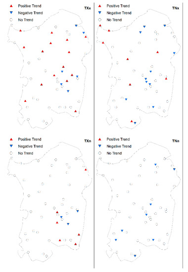
Figure 7.
Spatial distribution of extreme temperature indices trend (TXx, TNx, TXn and TNn; see Table 3 for abbreviation definitions).
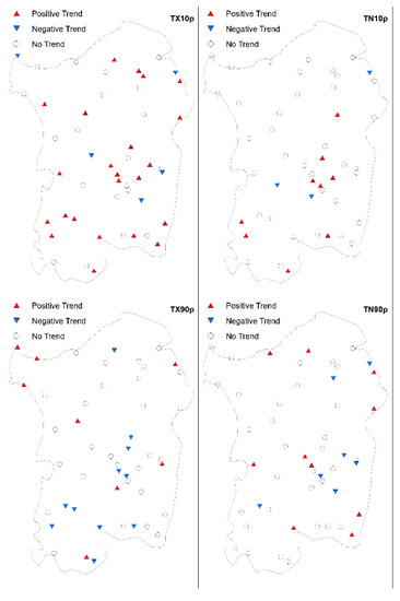
Figure 8.
Spatial distribution of extreme temperature indices trend (TX10p, TN10p, TX90p and TN90p; see Table 3 for abbreviation definitions).
On the contrary, a negative trend was detected in 25.0% (SL = 90%), 18.8% (SL = 95%) and 8.3% (SL = 99%) of the series especially in the southern part of the region (Figure 8). A more marked difference between positive and negative trends has been observed for TN10p and TX90p. In particular, for TN10p, 35.4% (18.8%), 29.2% (12.5%) and 10.4% (4.2%) of the series showed a positive (negative) trend with SLs of 90%, 95% and 99%, respectively (Figure 6). As regards TX90p, 58.3% (SL = 90%), 41.7% (SL = 95%) and 22.9% (SL = 99%) of the series showed a negative trend while only a maximum of 16.7% of the series showed a positive trend for an SL = 90% (Figure 6). The spatial analysis of the trend results for both TN10p and TX90p evidenced positive trends distributed across the region with few negative values in the central areas of the region (Figure 8). On the other hand, for the TN90p, a decreasing trend has been observed in more than 40% of the series, for SL = 90% and 95%, and in about 23% of the series for an SL = 99% (Figure 6), but also in this case no clear spatial patterns are visible in the region (Figure 8).
The analysis of the DTR index evidenced a marked increasing trend with 54.2% (SL = 90%), 47.9% (SL = 95%) and 41.7% (SL = 99%) of the series presenting positive values, and 22.9%, 10.4% and 6.3% of the series evidencing a negative trend for an SL equal to 90%, 95% and 99%, respectively (Figure 6). The spatial analysis of the trend results showed an almost uniform distribution of the positive trend across the region with few negative values in the central areas of the region (Figure 9). As regards the frost days (FD), 26.1%, 19.6% and 6.5% of the series showed a positive trend with an SL of 90%, 95% and 99%, respectively (Figure 6), mainly localized around the eastern mountain and in the southwestern side of the region (Figure 9). Conversely, a negative trend has been detected in 13.0% (SL = 90%) and 6.5% (SL = 95%). With respect to the summer days (SU25), a positive trend in 38.3% (SL = 90%), 27.7% (SL = 95%) and 17.0% (SL = 99%) and a negative trend in 23.4% (SL = 90%), 14.9% (SL = 95%) and 8.5% (SL = 99%) of the stations have been observed (Figure 6). Spatially, this evidence appears to be distributed all over the region without a clear difference between areas with positive or negative values (Figure 9).
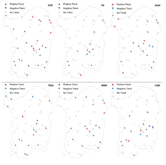
Figure 9.
Spatial distribution of extreme temperature indices trend (DTR, FD, SU25, TR20, WSDI and CSDI; see Table 3 for abbreviation definitions).
The tropical nights (TR20) show an almost equal number of positive and negative trends (Figure 6), with the latter mainly located in the southern part of the region (Figure 9). In particular, the percentage of negative trends ranges from 16.7% (SL = 99%) to 29.2% (SL = 90%) while the percentage of positive trends ranges from 12.5% (SL = 99%) to 22.9% (SL = 90%).
5. Discussion
Recently, a number of extreme climate indices, whether using observed, reanalysis, or climate projection data, have become available in the literature; however, small-scale analysis based on high-density networks are paramount to perform reliable analysis. As an example, in Italy, Zollo et al. [64] detected a general underestimation of both minimum and maximum temperature extremes for simulations driven by the CMCC–CM global model. They also found that for indices depending on maximum temperature, the spatial pattern is less skillfully represented in the case of regions characterized by a marked orography such as Calabria and Sardinia. Moreover, as evidenced by Kyselý and Plavcová [65] the E-OBS v2.0 gridded dataset shows large biases when compared to a high-density network. Within this context, although previous investigations on maximum and minimum temperatures at a planetary scale evidenced an increase in the minimum values rather than the maximum ones [66], results of this study evidenced an opposite behavior, thus confirming the findings achieved by previous research performed in Italy [41]. Similarly, these results only partially conform to the rising tendency identified since 1976 in warm days and nights in some European areas, and disagree with the weakness of the decreasing trends in cold days and nights [67]. Relating to diurnal temperature range (DTR), as verified in previous surveys, an important growing trend was detected due to a faster warming in maximum temperatures than in minimum ones, although some other DTR research works at a global scale proved an opposite behavior, showing a large decreasing trend [68,69,70,71]. In Sardinia, increasing frequency and intensity of warmer extremes, together with a weak increasing trend of the colder extremes, occurs. These outcomes agree with previous studies on daily temperature extremes in Mediterranean countries [42,48,72,73].
In accordance with the warming in global mean temperatures [1], a decrease in cold extremes and an increase in warm ones has occurred since the middle of the twentieth century in a vast majority of land regions. In Europe, this trend has been already experienced since 1960 [74], when a statistically significant increase in the number of warm days and nights, and an opposite trend in the number of cold days and nights, have been detected. However, there is no agreement in the literature on trend behavior, and differing tendencies for temperature extremes have been recognized over different time-periods during the last century [14,75].
6. Conclusions
The temporal variability assessment of monthly and extreme temperatures in the Sardinia region (Italy) was carried out to identify the trends, and to analyze the behaviors of the extreme temperatures, in the period 1922–2011, by means of 14 commonly used daily temperature indices. From this analysis we draw some important concluding remarks:
- (a)
- For the minimum temperature series, diffuse negative tendencies have been identified, with a positive trend observed only in the spring months;
- (b)
- For the maximum temperature series, a general increasing trend has been identified in almost all the months, with the exclusion of January, September, December and, partially, October. In particular, a consistent positive trend in the spring and in the summer months has been detected, especially in June;
- (c)
- Among the evaluation of the indices of extreme temperatures, the DTR results evidenced a marked increasing trend distributed across the region. The frost days (FD) showed a positive trend of the series mainly localized around the eastern mountain and in the southwestern side of the region. The summer days (SU25) displayed more positive trends than negative ones, spatially distributed all over the region. The tropical nights (TR20) showed an equal distribution of positive and negative trends. Finally, both the warm (WSDI) and the cold (CSDI) spell indices displayed an increasing trend localized in the southern part of the region.
- (d)
- Results indicate that Sardinia’s topography may cause temperature variability. In fact, the mountains crossing the island constitute a barrier between the tropical air masses coming from the African coasts on eastern side, and air masses carried by western winds originating from the Atlantic Ocean on the western side. The changes in the temperature regime in this region could have regionally specific impacts on its ecosystems.
- (e)
- These results can be very useful for several stakeholders. In particular: (i) planners, disaster management agencies and policy makers who need to be alert in a region with a high-density population; (ii) hydrologists and climatologists who need to investigate the potential causes of the observed temporal trends to delineate the variability of extremes due to natural and anthropogenic effects.
Author Contributions
Conceptualization, T.C. and I.G.; methodology, T.C.; software, T.C.; validation, T.C. and I.G.; formal analysis, T.C.; investigation, I.G.; resources, T.C. and I.G.; data curation, I.G.; writing—original draft preparation, T.C. and I.G.; writing—review and editing, T.C. and I.G.; visualization, T.C. and I.G.; supervision, T.C. All authors have read and agreed to the published version of the manuscript.
Funding
This research received no external funding.
Conflicts of Interest
The authors declare no conflict of interest.
References
- IPCC. Summary for Policymakers. Fifth Assessment Report of the Intergovernmental Panel on Climate Change; Cambridge University Press: Cambridge, UK, 2013. [Google Scholar]
- Tol, R.S.J. Population and trends in the global mean temperature. Atmósfera 2017, 30, 121–135. [Google Scholar] [CrossRef]
- Folland, C.K.; Boucher, O.; Colman, A.; Parker, D.E. Causes of irregularities in trends of global mean surface temperature since the late 19th century. Sci. Adv. 2018, 4, eaao5297. [Google Scholar] [CrossRef] [PubMed]
- Mahmoudi, P.; Mohammadi, M.; Daneshmand, H. Investigating the trend of average changes of annual temperatures in Iran. Int. J. Environ. Sci. Technol. 2019, 16, 1079–1092. [Google Scholar] [CrossRef]
- Salman, S.A.; Shahid, S.; Ismail, T.; Ahmed, K.; Chung, E.S.; Al-Abadi, A.M. Long-term trends in daily temperature extremes in Iraq. Atmos. Res. 2018, 198, 97–107. [Google Scholar] [CrossRef]
- Sirangelo, B.; Caloiero, T.; Coscarelli, R.; Ferrari, E. A stochastic model for the analysis of maximumdaily temperature. Theor. Appl. Climatol. 2017, 130, 275–289. [Google Scholar] [CrossRef]
- Pellicone, G.; Caloiero, T.; Guagliardi, I. The De Martonne aridity index in Calabria (Southern Italy). J. Maps 2019, 15, 788–796. [Google Scholar] [CrossRef]
- Pellicone, G.; Caloiero, T.; Modica, G.; Guagliardi, I. Application of several spatial interpolation techniques to monthly rainfall data in the Calabria region (southern Italy). Int. J. Climatol. 2018, 38, 3651–3666. [Google Scholar] [CrossRef]
- Cao, L.; Zhang, Y.; Shi, Y. Climate change effect on hydrological processes over the Yangtze River basin. Quat. Int. 2011, 244, 202–210. [Google Scholar] [CrossRef]
- Keellings, D.; Waylen, P. The stochastic properties of high daily maximum temperatures applying crossing theory to modelling high-temperature event variables. Theor. Appl. Climatol. 2012, 108, 579–590. [Google Scholar] [CrossRef]
- Munich, R. TOPICS Geo 2003; Münchener Rückverischerungs-Gessellschaft: Munich, Germany, 2004. [Google Scholar]
- García-Herrera, R.; Díaz, J.; Trigo, R.M.; Luterbacher, J.; Fischer, E.M. A Review of the European Summer Heat Wave of 2003. Crit. Rev. Environ. Sci. Technol. 2010, 40, 267–306. [Google Scholar] [CrossRef]
- UNEP. The European Summer Heat Wave of 2003; United Nations Environmental Programme: Nairobi, Kenya, 2004. [Google Scholar]
- Buttafuoco, G.; Caloiero, T.; Ricca, N.; Guagliardi, I. Assessment of drought and its uncertainty in a southern Italy area (Calabria region). Measurement 2018, 113, 205–210. [Google Scholar] [CrossRef]
- Buttafuoco, G.; Caloiero, T.; Guagliardi, I.; Ricca, N. Drought assessment using the reconnaissance drought index (RDI) in a southern Italy region. In Proceedings of the 6th IMEKO TC19 Symposium on Environmental Instrumentation and Measurements, Reggio Calabria, Italy, 24–25 June 2016; pp. 52–55. [Google Scholar]
- Ricca, N.; Guagliardi, I. Multi-temporal dynamics of land use patterns in a site of community importance in Southern Italy. Appl. Ecol. Environ. Res. 2015, 13, 677–691. [Google Scholar]
- Cornes, R.; van der Schrier, G.; van den Besselaar, E.J.M.; Jones, P.D. An Ensemble Version of the E-OBS Temperature and Precipitation Datasets. J. Geophys. Res. Atmos. 2018, 123, 9391–9409. [Google Scholar] [CrossRef]
- Mistry, M.N. A High-Resolution Global Gridded Historical Dataset of Climate Extreme Indices. Data 2019, 4, 41. [Google Scholar] [CrossRef]
- Moberg, A.; Jones, P.D. Trends in indices for extremes in daily temperature and precipitation in central and western Europe analyzed 1901–1999. Int. J. Climatol. 2005, 2, 1149–1171. [Google Scholar] [CrossRef]
- Croitoru, A.E.; Piticar, A. Changes in daily extreme temperatures in the extra-Carpathians regions of Romania. Int. J. Climatol. 2013, 33, 1987–2001. [Google Scholar] [CrossRef]
- Toll, V.; Post, P. Daily temperature and precipitation extremes in the Baltic Sea region derived from the BaltAn65+ reanalysis. Theor. Appl. Climatol. 2018, 132, 647–662. [Google Scholar] [CrossRef]
- Insaf, T.Z.; Lin, S.; Sheridan, S.C. Climate trends in indices for temperature and precipitation across New York state, 1948–2008. Air Qual. Atmos. Health 2012, 6, 247–257. [Google Scholar] [CrossRef]
- Lopez-Franca, N.; Zaninelli, P.G.; Caril, A.F.; Menendez, C.G.; Sanchez, E. Changes in temperature extremes for 21st century scenarios over South America derived from a multi-model ensemble of regional climate models. Clim. Res. 2016, 68, 151–167. [Google Scholar] [CrossRef]
- Meseguer-Ruiz, O.; Ponce-Philimon, P.I.; Quispe-Jofré, A.S.; Guijarro, J.A.; Sarricolea, P. Spatial behaviour of daily observed extreme temperatures in Northern Chile (1966-2015): Data quality, warming trends, and its orographic and latitudinal effects. Stoch. Environ. Res. Risk Assess. 2018, 32, 3503–3523. [Google Scholar] [CrossRef]
- Shen, X.; Liu, B.; Lu, X.; Fan, G. Spatial and temporal changes in daily temperature extremes in China during 1960–2011. Theor. Appl. Climatol. 2017, 130, 933–943. [Google Scholar] [CrossRef]
- Chen, A.; He, X.; Guan, H.; Cai, Y. Trends and periodicity of daily temperature and precipitation extremes during 1960–2013 in Hunan Province, central south China. Theor. Appl. Climatol. 2018, 132, 71–88. [Google Scholar] [CrossRef]
- Caloiero, T. The trend of monthly temperature and daily extreme temperature during 1951–2012 in New Zealand. Theor. Appl. Climatol. 2017, 129, 111–127. [Google Scholar] [CrossRef]
- Shrestha, A.B.; Bajracharya, S.R.; Sharma, A.R.; Duo, C.; Kulkarni, A. Observed trends and changes in daily temperature and precipitation extremes over the Koshi river basin 1975–2010. Int. J. Climatol. 2017, 37, 1066–1083. [Google Scholar] [CrossRef]
- Chakraborty, D.; Sehgal, V.K.; Dhakar, R.; Varghese, E.; Das, D.K.; Ray, M. Changes in daily maximum temperature extremes across India over 1951–2014 and their relation with cereal crop productivity. Stoch. Environ. Res. Risk Assess. 2018, 32, 3067–3081. [Google Scholar] [CrossRef]
- Dimri, A.P. Comparison of regional and seasonal changes and trends in daily surface temperature extremes over India and its subregions. Theor. Appl. Climatol. 2019, 136, 265–286. [Google Scholar] [CrossRef]
- Filahi, S.; Tanarhte, M.; Mouhir, L.; El Morhit, M.; Tramblay, Y. Trends in indices of daily temperature and precipitations extremes in Morocco. Theor. Appl. Climatol. 2016, 124, 959–972. [Google Scholar] [CrossRef]
- Halimatou, A.T.; Kalifa, T.; Kyei-Baffour, N. Assessment of changing trends of daily precipitation and temperature extremes in Bamako and Ségou in Mali from 1961-2014. Weather Clim. Extrem. 2017, 18, 8–16. [Google Scholar] [CrossRef]
- Salman, S.A.; Shahid, S.; Ismail, T.; Ahmed, K.; Chung, E.S.; Wang, X.J. Characteristics of Annual and Seasonal Trends of Rainfall and Temperature in Iraq. Asia-Pac. J. Atmos. Sci. 2019, 55, 429–438. [Google Scholar] [CrossRef]
- Giorgi, F. Climate change hot-spots. Geophys. Res. Lett. 2006, 33, L08707. [Google Scholar] [CrossRef]
- Hertig, E.; Seubert, S.; Jacobeit, J. Temperature extremes in the Mediterranean area: Trends in the past and assessments for the future. Nat. Hazards Earth Syst. Sci. 2010, 10, 2039–2050. [Google Scholar] [CrossRef]
- Efthymiadis, D.; Goodess, C.M.; Jones, P.D. Trends in Mediterranean gridded temperature extremes and large-scale circulation influences. Nat. Hazards Earth Syst. Sci. 2011, 11, 2199–2214. [Google Scholar] [CrossRef]
- Brunetti, M.; Maugeri, M.; Monti, F.; Nanni, T. Temperature and precipitation variability in Italy in the last two centuries from homogenised instrumental time series. Int. J. Climatol. 2006, 26, 345–381. [Google Scholar] [CrossRef]
- Colombo, T.; Pelino, V.; Vergari, S.; Cristofanelli, P.; Bonasoni, P. Study of temperature and precipitation variations in Italy based on surface instrumental observations. Glob. Planet. Chang. 2007, 57, 308–318. [Google Scholar] [CrossRef]
- Ciccarelli, N.; Von Hardenberg, J.; Provenzale, A.; Ronchi, C.; Vargiu, A.; Pelosini, R. Climate variability in north-western Italy during the second half of the 20th century. Glob. Planet. Chang. 2008, 63, 185–195. [Google Scholar] [CrossRef]
- Pellicone, G.; Caloiero, T.; Coletta, V.; Veltri, A. Phytoclimatic map of Calabria (Southern Italy). J. Maps 2014, 10, 109–113. [Google Scholar] [CrossRef]
- Caloiero, T.; Buttafuoco, G.; Coscarelli, R.; Ferrari, E. Spatial and temporal characterization of climate at regional scale using homogeneous monthly precipitation and air temperature data: An application in Calabria (Southern Italy). Hydrol. Res. 2015, 46, 629–646. [Google Scholar] [CrossRef]
- Caloiero, T.; Callegari, G.; Cantasano, N.; Coletta, V.; Pellicone, G.; Veltri, A. Bioclimatic analysis in a region of southern Italy (Calabria). Plant Biosyst. 2015, 150, 1282–1295. [Google Scholar] [CrossRef]
- Sirangelo, B.; Caloiero, T.; Coscarelli, R.; Ferrari, E. A combined stochastic analysis of mean daily temperature and diurnal temperature range. Theor. Appl. Climatol. 2019, 135, 1349–1359. [Google Scholar] [CrossRef]
- Toreti, A.; Desiato, F. Temperature trend over Italy from 1961 to 2004. Theor. Appl. Climatol. 2008, 91, 51–58. [Google Scholar] [CrossRef]
- Simolo, C.; Brunetti, M.; Maugeri, M.; Nanni, T.; Speranza, A. Understanding climate change-induced variations in daily temperature distributions over Italy. J. Geophys. Res. Atmos. 2010, 115, D22110. [Google Scholar] [CrossRef]
- Acquaotta, F.; Fratianni, S.; Garzena, D. Temperature changes in the North-Western Italian Alps from 1961 to 2010. Theor. Appl. Climatol. 2015, 122, 619–634. [Google Scholar] [CrossRef]
- Tomozeiu, R.; Pavan, V.; Cacciamani, C.; Amici, M. Observed temperature changes in Emilia-Romagna: Mean values and extremes. Clim. Res. 2006, 31, 217–225. [Google Scholar] [CrossRef]
- Scorzini, A.R.; Di Bacco, M.; Leopardi, M. Recent trends in daily temperature extremes over the central Adriatic region of Italy in a Mediterranean climatic context. Int. J. Climatol. 2018, 38, e741–e757. [Google Scholar] [CrossRef]
- Bartolini, G.; Di Stefano, V.; Maracchi, G.; Orlandini, S. Mediterranean warming is especially due to summer season. Evidences from Tuscany (central Italy). Theor. Appl. Climatol. 2012, 107, 279–295. [Google Scholar] [CrossRef]
- Piccarreta, M.; Lazzari, M.; Pasini, A. Trends in daily temperature extremes over the Basilicata region (southern Italy) from 1951 to 2010 in a Mediterranean climatic context. Int. J. Climatol. 2015, 35, 1964–1975. [Google Scholar] [CrossRef]
- Caloiero, T.; Coscarelli, R.; Ferrari, E.; Sirangelo, B. Trend analysis of monthly mean values and extreme indices of daily temperature in a region of southern Italy. Int. J. Climatol. 2017, 37, 284–297. [Google Scholar] [CrossRef]
- Mann, H.B. Nonparametric tests against trend. Econom. J. Conom. Soc. 1945, 13, 245–259. [Google Scholar] [CrossRef]
- Kendall, M.G. Rank Correlation Methods; Hafner Publishing Company: New York, NY, USA, 1962. [Google Scholar]
- Montaldo, N.; Sarigu, A. Potential links between the North Atlantic Oscillation and decreasing precipitation and runoff on a Mediterranean area. J. Hydrol. 2017, 553, 419–437. [Google Scholar] [CrossRef]
- Beck, H.E.; Zimmermann, N.E.; McVicar, T.R.; Vergopolan, N.; Berg, A.; Wood, E.F. Present and future Köppen-Geiger climate classification maps at 1-km resolution. Sci Data 2018, 5, 180214. [Google Scholar] [CrossRef]
- Regione Sardegna. Available online: http://www.regione.sardegna.it/j/v/25?s=131338&v=2&c=5650&t=1 (accessed on 28 July 2020).
- Caloiero, T.; Coscarelli, R.; Gaudio, R. Spatial and temporal variability of daily precipitation concentration in the Sardinia region (Italy). Int. J. Climatol. 2019, 39, 5006–5021. [Google Scholar] [CrossRef]
- Caloiero, T.; Coscarelli, R.; Gaudio, R.; Leonardo, G.P. Precipitation trend and concentration in the Sardinia region. Theor. Appl. Climatol. 2019, 137, 297–307. [Google Scholar] [CrossRef]
- Caloiero, T.; Veltri, S. Drought assessment in the Sardinia region (Italy) during 1922–2011 using the standardized precipitation index. Pure Appl. Geophys. 2019, 176, 925–935. [Google Scholar] [CrossRef]
- Barrera-Escoda, A.; Gonçalves, M.; Guerreiro, D.; Cunillera, J.; Baldasano, J.M. Projections of temperature and precipitation extremes in the North Western Mediterranean Basin by dynamical downscaling of climate scenarios at high resolution (1971–2050). Clim. Chang. 2014, 122, 567–582. [Google Scholar] [CrossRef]
- Fioravanti, G.; Piervitali, E.; Desiato, F. Recent changes of temperature extremes over Italy: And index-based analysis. Theor. Appl. Climatol. 2016, 123, 473–486. [Google Scholar] [CrossRef]
- El Kenawy, A.M.; Lopez-Moreno, J.I.; McCabe, M.F.; Robaa, S.M.; Domínguez-Castro, F.; Peña-Gallardo, M.; Trigo, R.M.; Hereher, M.E.; Al-Awadhi, T.; Vicente-Serrano, S.M. Daily temperature extremes over Egypt: Spatial patterns, temporal trends, and driving forces. Atmos. Res. 2019, 226, 219–239. [Google Scholar] [CrossRef]
- Zhang, X.; Alexander, L.; Hegerl, G.C.; Jones, P.; Tank, A.K.; Peterson, T.C.; Trewin, B.; Zwiers, F.W. Indices for monitoring changes in extremes based on daily temperature and precipitation data. Clim. Chang. 2011, 2, 851–887. [Google Scholar] [CrossRef]
- Zollo, A.L.; Rillo, V.; Bucchignani, E.; Montesarchio, M.; Mercogliano, P. Extreme temperature and precipitation events over Italy: Assessment of high-resolution simulations with COSMO-CLM and future scenarios. Int. J. Climatol. 2016, 36, 987–1004. [Google Scholar] [CrossRef]
- Kyselý, J.; Plavcová, E. A critical remark on the applicability of E-OBS European gridded temperature data set for validating control climate simulations. J. Geophys. Res. 2010, 115, D23118. [Google Scholar]
- Easterling, D.R.; Horton, B.; Jones, P.D.; Peterson, T.C.; Karl, T.R.; Parker, D.E.; Salinger, M.J.; Razuvayev, V.; Plummer, N.; Jamason, P.; et al. Maximum and minimum temperature trends for the globe. Science 1997, 277, 364–367. [Google Scholar] [CrossRef]
- Bartholy, J.; Pongrácz, R. Regional analysis of extreme temperature and precipitation indices for the Carpathian Basin from 1946 to 2001. Glob. Planet. Chang. 2007, 57, 83–95. [Google Scholar] [CrossRef]
- Wild, M.; Ohmura, A.; Makowski, K. Impact of global dimming and brightening on global warming. Geophys. Res. Lett. 2007, 34, L04702. [Google Scholar] [CrossRef]
- Vose, R.S.; Easterling, D.R.; Gleason, B. Maximum and minimum temperature trends for the globe: An update through 2004. Geophys. Res. Lett. 2005, 32, L23824. [Google Scholar] [CrossRef]
- Rohde, R.; Muller, R.; Jacobsen, R.; Perlmutter, S.; Rosenfeld, A.; Wurtele, J.; Curry, J.; Wickhams, C.; Mosher, S. Berkeley Earth temperature averaging process. Geoinf. Geostat. Overv. 2013, 1, 1–13. [Google Scholar] [CrossRef]
- Guan, Y.; Zhang, X.; Zheng, F.; Wang, B. Trends and variability of daily temperature extremes during 1960–2012 in the Yangtze River Basin, China. Glob. Planet. Chang. 2015, 124, 79–94. [Google Scholar] [CrossRef]
- El Kenawy, A.; López-Moreno, J.I.; Vicente-Serrano, S.M. Recent trends in daily temperature extremes over northeastern Spain (1960–2006). Nat. Hazards Earth Syst. Sci. 2011, 11, 2583–2603. [Google Scholar] [CrossRef]
- Ramos, A.M.; Trigo, R.M.; Santo, F.E. Evolution of extreme temperatures over Portugal: Recent changes and future scenarios. Clim. Res. 2011, 48, 177–192. [Google Scholar] [CrossRef]
- EEA. Climate Change, Impacts and Vulnerability in Europe 2012, an Indicator-Based Report; EEA Report, No. 12/2012; European Environment Agency (EEA): Copenhagen, Denmark, 2012. [Google Scholar]
- Klein Tank, A.M.G.; Konnen, G.P. Trends in indices of daily temperature and precipitation extremes in Europe, 1946–1999. J. Clim. 2003, 16, 3665–3680. [Google Scholar] [CrossRef]


© 2020 by the authors. Licensee MDPI, Basel, Switzerland. This article is an open access article distributed under the terms and conditions of the Creative Commons Attribution (CC BY) license (http://creativecommons.org/licenses/by/4.0/).