
Impacts of Climate Change on Irrigation Water Management in the Babai River Basin, Nepal


Abstract
:1. Introduction
2. Data and Method
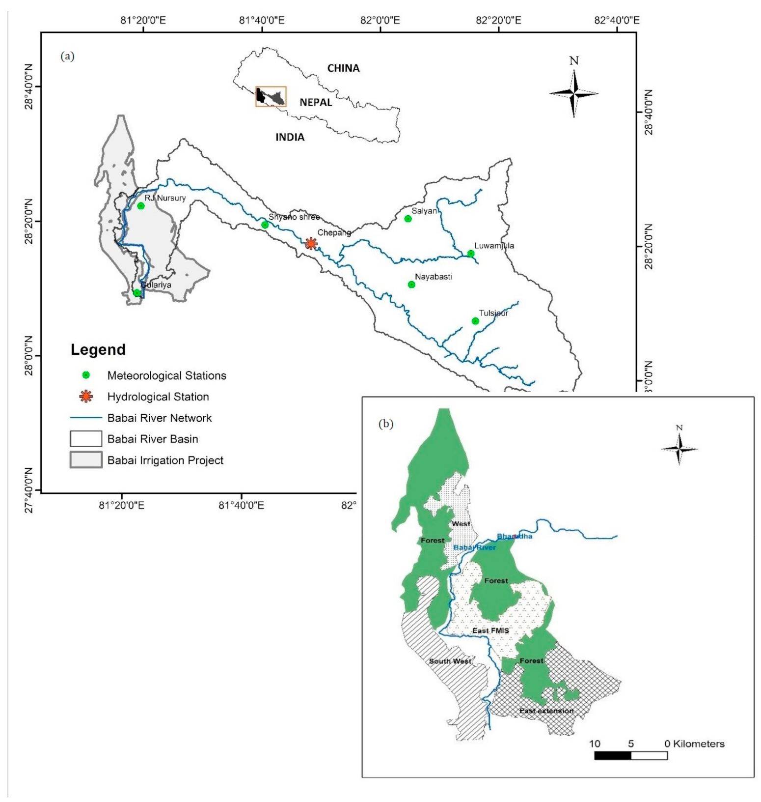
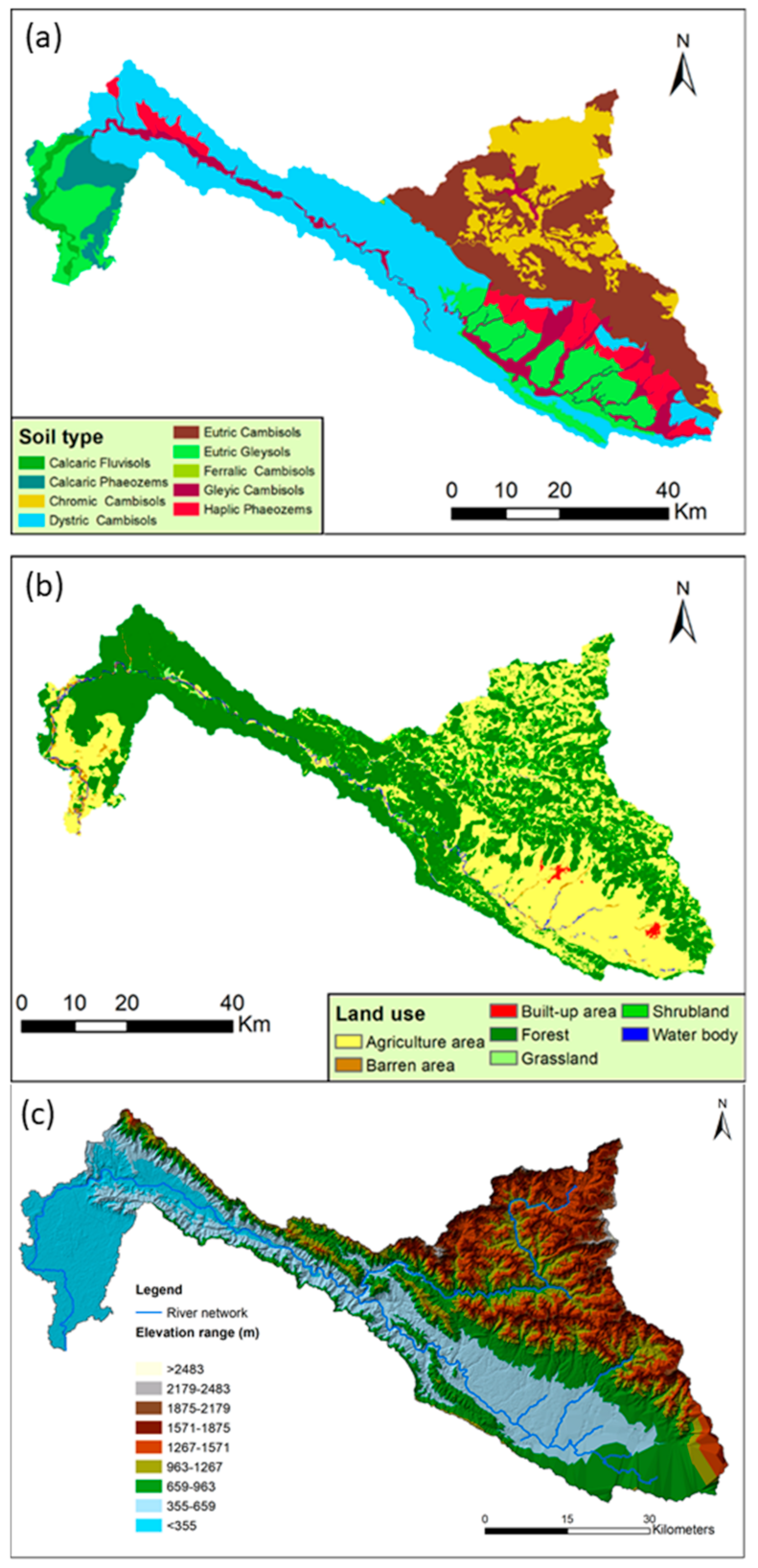
2.1. Study Area
2.2. Data Sources
2.2.1. Digital Elevation Model
2.2.2. Soil and Land Cover Data
2.2.3. Streamflow and Meteorological Data
2.2.4. Global Climate Model Data
2.2.5. Cropping Patterns
2.3. Methods
2.3.1. Bias Correction of RCP Scenario Data
2.3.2. SWAT Model Setup, Calibration, and Validation
2.3.3. CROPWAT Model
2.3.4. Environmental Flow Calculator (EFC)
3. Results and Discussion
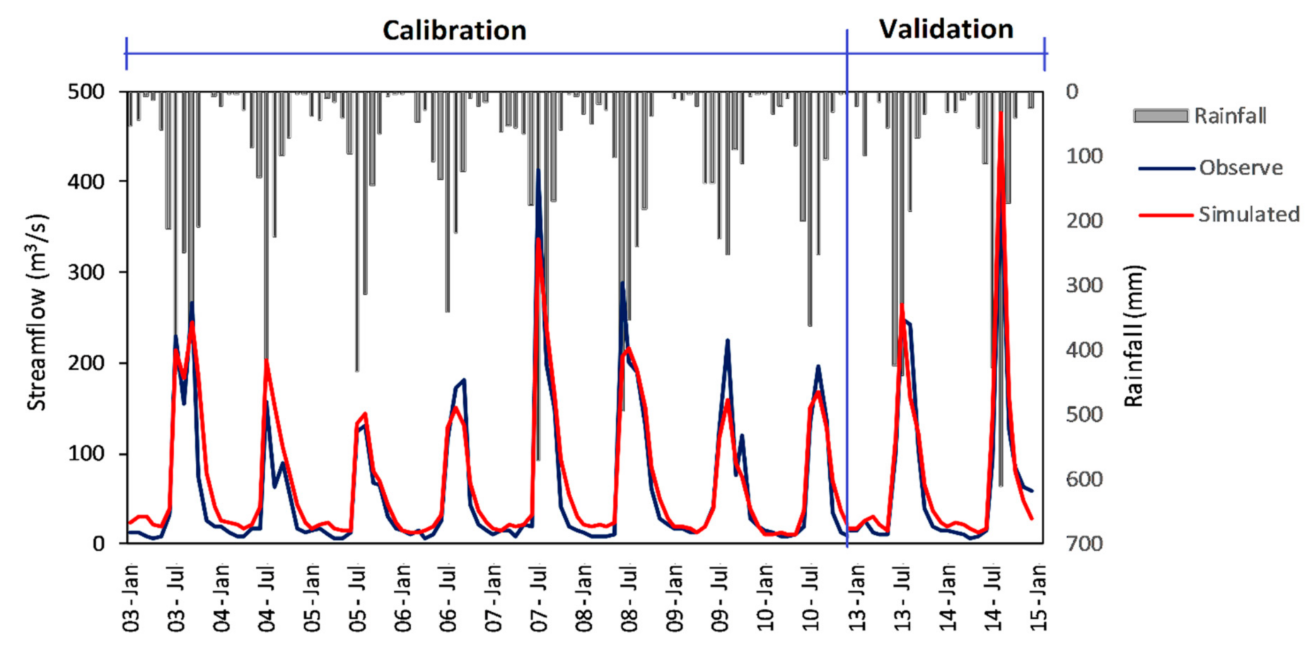
3.1. Calibration and Validation of the Model
3.2. Water Budget during the Calibration and Validation Periods
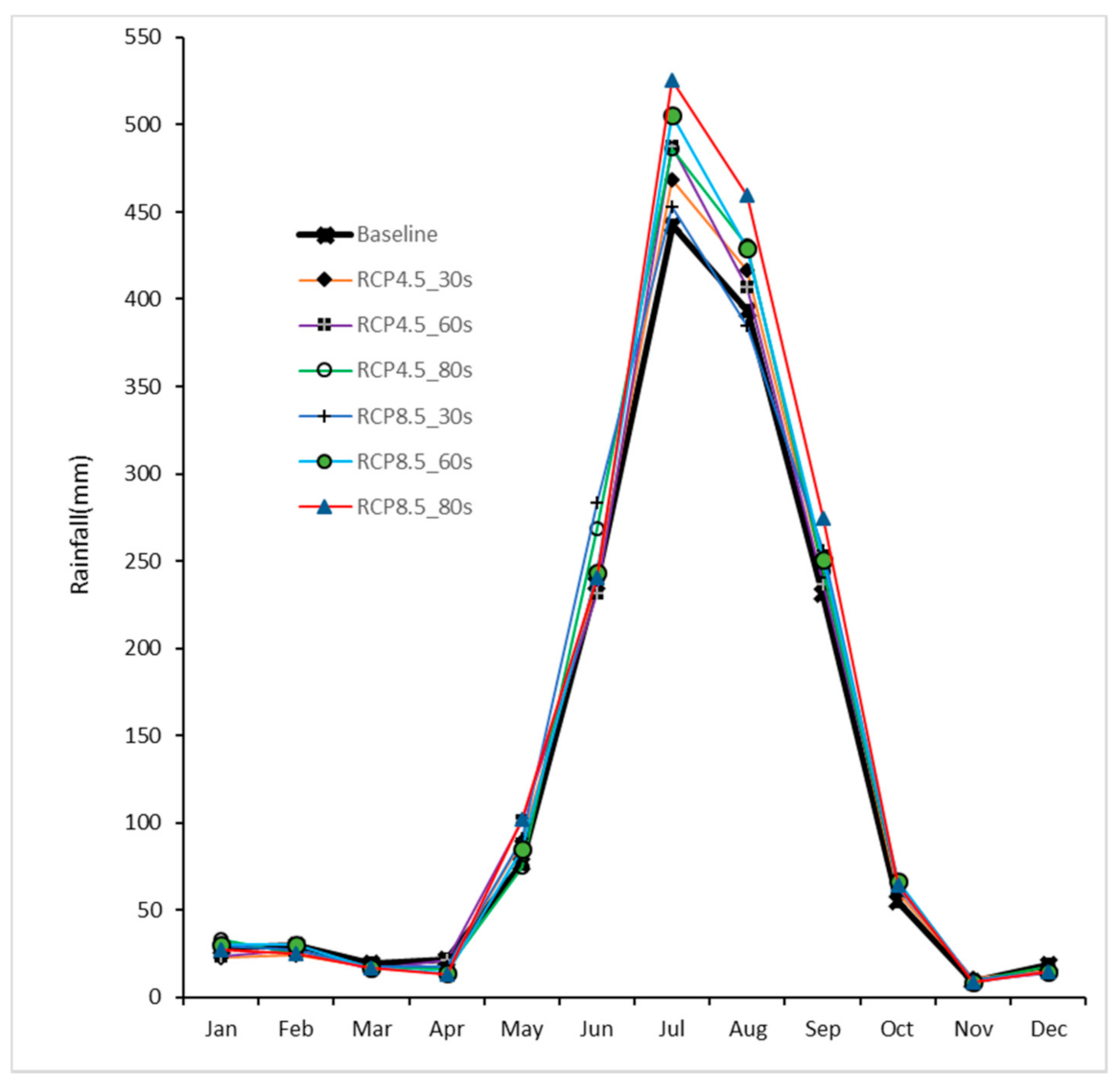
3.3. Climate Change Scenario Generation
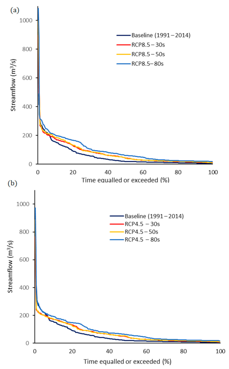
3.4. Climate Change Impact on Streamflow
3.5. Irrigation Water Demand in the Babai River Basin
3.6. Environment Flow
3.7. Water Deficit and Surplus Scenario
3.8. Discussion and Summary
4. Conclusions
- (a)
- The SWAT model was calibrated and validated for the Babai River Basin. For monthly calibration, the model performed well with R2 at 0.89 and NSE at 0.88 and +14.5% for PBIAS in the calibration period and R2 at 0.93 and NSE at 0.92, and PBIAS +10.9% for the validation period.
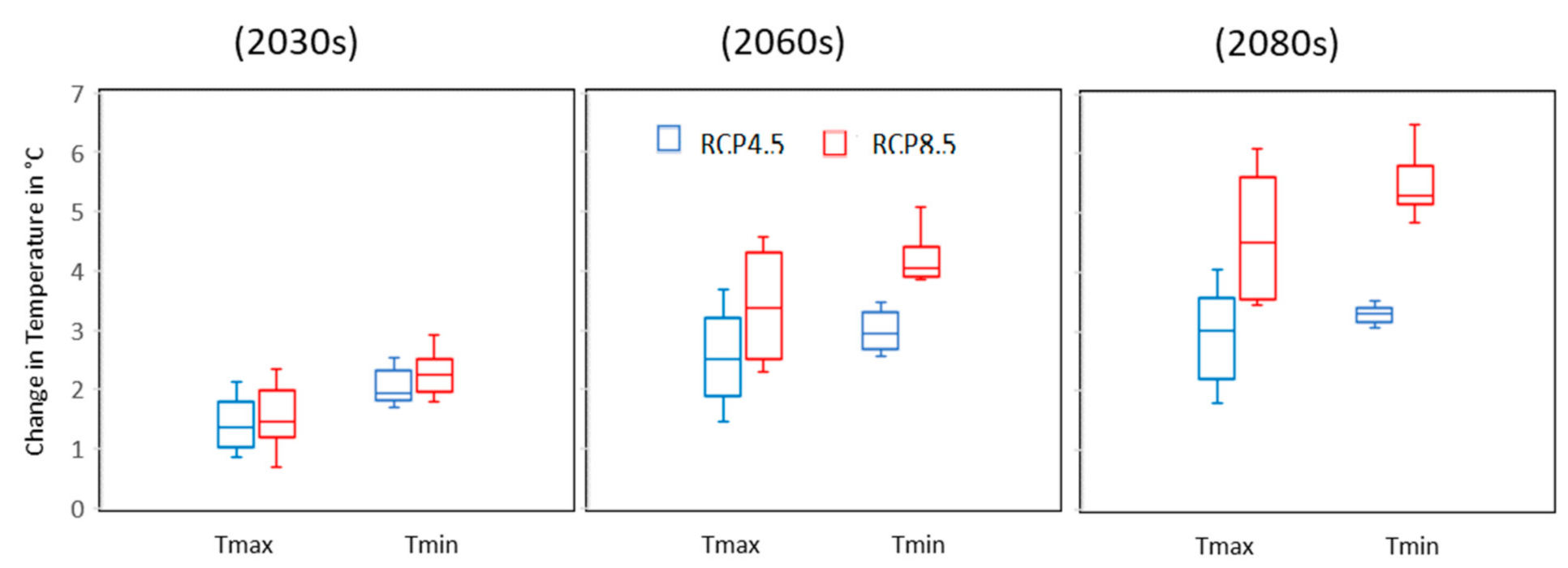
- (b)
- The pattern of future rainfall is similar to the baseline period but an increment is predicted. Future annual rainfall is expected to increase by 15% to 25% as compared to the baseline period. The maximum increment is under RCP 8.5 in the 2080s and the minimum increment is under RCP 4.5 in the 2030s. The minimum and maximum temperatures also increase in the future by around 2 to 4.5 °C, as compared to the baseline period.
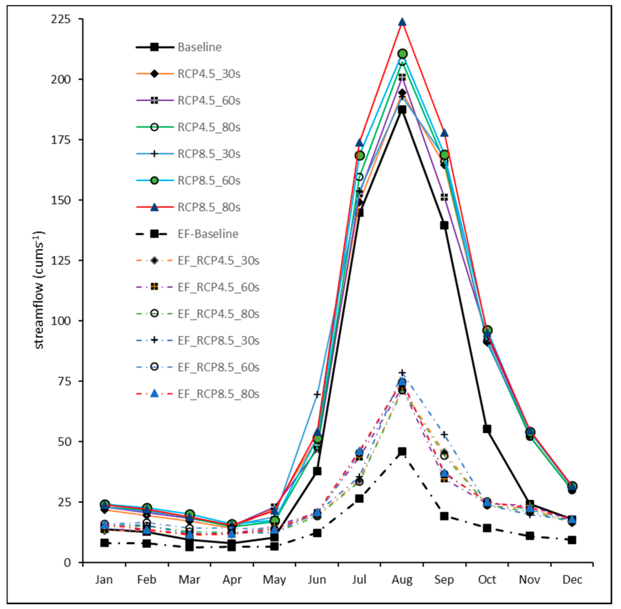
- (c)
- The consequences of increased rainfall and temperature reflect in the streamflow. It can be predicted that annual streamflow will rise by 24–27% under RCP 4.5 and 28–37% under RCP 8.5, while monthly increments can go up to 75% in February. As per the flow duration curve, the probability of occurrence of flow and magnitude of flow could be higher in the future than in the baseline period under both scenarios.
- (d)
- EF was calculated corresponding to EMC and the results show that EF varies from 20 to 88% of the natural flow.
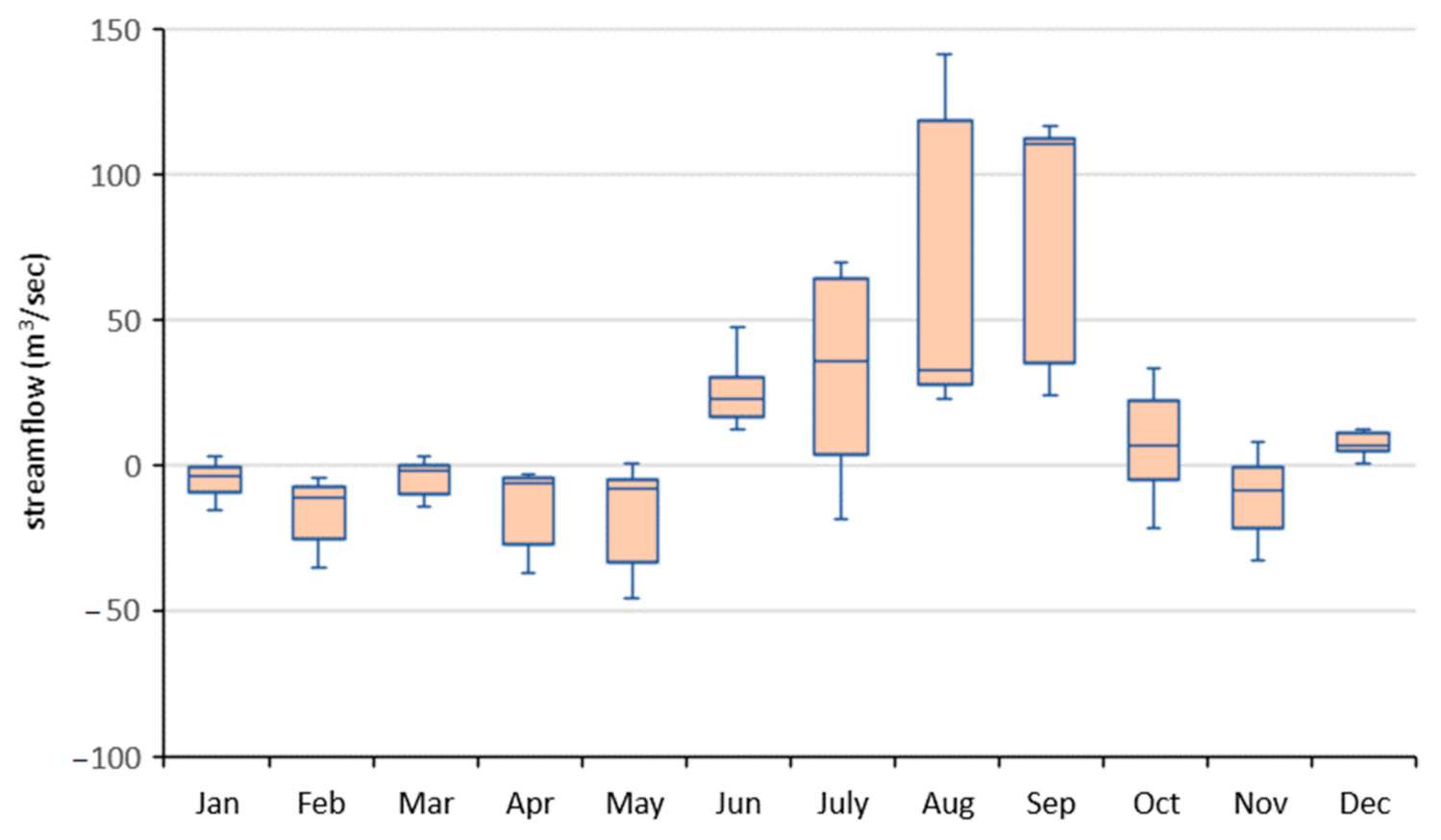
- (e)
- Demand for water in the Babai River Basin will increase in the future due to changing cropping patterns. Although rainfall is predicted to increase in the future, this incremental rainfall will not be sufficient to meet the increasing demand. Under current conditions, water deficit is seen in six months and the maximum water deficit is in November (around 33.07 m3/s). The water balance breaks even in January and March. Under the CC condition of the present CI, the IWD will decrease. However, as per the BIP, cropping intensity is to increase to 250%, and under all scenarios, water could be scarcer for five months of the year: from January to May. The maximum shortage is expected in May, followed by April, February, March, and January. Hence, all these results indicate that the water available in the Babai River is not sufficient now and will not be in the future to supply to the year-round irrigation system and sustain a fresh ecosystem. Alternative sources of water are essential and must be deployed at the earliest. Until managing the alternative sources of water, we recommend cultivating less water-demand crops such as wheat and maize instead of rice and sugarcane.
Supplementary Materials
Author Contributions
Funding
Acknowledgments
Conflicts of Interest
References
- Mishra, Y.; Nakamura, T.; Babel, M.S.; Ninsawat, S.; Ochi, S. Impact of Climate Change on Water Resources of the Bheri River Basin, Nepal. Water 2018, 10, 220. [Google Scholar] [CrossRef] [Green Version]
- IPCC AR5—Summary for Policymakers. Contribution of Working Group I to the Fifth Assessment Report of the Intergovernmental Panel on Climate Change. In Climate Change 2013: The Physical Science Basis; Cambridge University Press: Cambridge, UK; New York, NY, USA, 2013; p. 78. [Google Scholar] [CrossRef] [Green Version]
- Shrestha, A.B.; Wake, C.P.; Mayewski, P.A.; Dibb, J.E. Precipitation fluctuations in the Himalaya and its vicinity: An analysis based on temperature records from Nepal. Int. J. Clim. 2000, 20, 317–327. [Google Scholar] [CrossRef]
- Babel, M.S.; Bhusal, S.P.; Wahid, S.M.; Agarwal, A. Climate change and water resources in the Bagmati River Basin, Nepal. Theor. Appl. Climatol. 2014, 115, 639–654. [Google Scholar] [CrossRef]
- Mishra, B.; Babel, M.S.; Tripathi, N.K. Analysis of climatic variability and snow cover in the Kaligandaki River Basin, Himalaya, Nepal. Theor. Appl. Clim. 2014, 116, 681–694. [Google Scholar] [CrossRef]
- Krishnamurthy, C.K.B.; Lall, U.; Kwon, H.H. Changing frequency and intensity of rainfall extremes over India from 1951 to 2003. J. Clim. 2009, 22, 4737–4746. [Google Scholar] [CrossRef] [Green Version]
- Tambe, S.; Kharel, G.; Arrawatia, M.L.; Kulkarni, H.; Mahamuni, K.; Ganeriwala, A.K. Reviving Dying Springs: Climate Change Adaptation Experiments From the Sikkim Himalaya. Mt. Res. Dev. 2012, 32, 62–72. [Google Scholar] [CrossRef]
- Negi, G.C.S.; Joshi, V. Rainfall and spring discharge patterns in two small drainage catchments in the western Himalayan Mountains, India. Environmentalist 2004, 24, 19–28. [Google Scholar] [CrossRef]
- Bookhagen, B.; Burbank, D.W. Toward a complete Himalayan hydrological budget: Spatiotemporal distribution of snowmelt and rainfall and their impact on river discharge. J. Geophys. Res. Earth Surf. 2010, 115, 1–25. [Google Scholar] [CrossRef] [Green Version]
- Erdogan, R. Stakeholder Involvement in Sustainable Watershed Management. Adv. Landsc. Archit. 2013. [Google Scholar] [CrossRef] [Green Version]
- Bhatta, L.D.; Van Oort, B.E.H.; Rucevska, I.; Baral, H. Payment for ecosystem services: Possible instrument for managing ecosystem services in Nepal. Int. J. Biodivers. Sci. Ecosyst. Serv. Manag. 2014, 10, 289–299. [Google Scholar] [CrossRef]
- Ouyang, F.; Zhu, Y.; Fu, G.; Lü, H.; Zhang, A.; Yu, Z.; Chen, X. Impacts of climate change under CMIP5 RCP scenarios on streamflow in the Huangnizhuang catchment. Stoch. Environ. Res. Risk Assess. 2015, 29, 1781–1795. [Google Scholar] [CrossRef]
- Arnold, J.G.; Srinivasan, R.; Muttiah, R.S.; Williams, J.R. Large area hydrologic modeling and assessment Part I: Model development. JAWRA J. Am. Water Resour. Assoc. 1998, 34, 73–89. [Google Scholar] [CrossRef]
- Kiros, G.; Shetty, A.; Nandagiri, L. Performance Evaluation of SWAT Model for Land Use and Land Cover Changes under different Climatic Conditions: A Review. J. Waste Water Treat. Anal. 2015, 6. [Google Scholar] [CrossRef]
- Smakhtin, V.U.; Eriyagama, N. Environmental Modelling & Software Developing a software package for global desktop assessment of environmental flows. Environ. Model. Softw. 2008, 23, 1396–1406. [Google Scholar] [CrossRef]
- Uddin, K.; Shrestha, H.L.; Murthy, M.S.R.; Bajracharya, B.; Shrestha, B.; Gilani, H.; Pradhan, S.; Dangol, B. Development of 2010 national land cover database for the Nepal. J. Environ. Manag. 2015, 148, 82–90. [Google Scholar] [CrossRef]
- Shrestha, S.; Shrestha, M.; Babel, M.S. Assessment of climate change impact on water diversion strategies of Melamchi Water Supply Project in Nepal. Theor. Appl. Climatol. 2017, 128, 311–323. [Google Scholar] [CrossRef]
- Mishra, B.; Tripathi, N.K.; Babel, M.S. An artificial neural network-based snow cover predictive modeling in the higher Himalayas. J. Mt. Sci. 2014, 11, 825–837. [Google Scholar] [CrossRef]
- Arnold, J.G.; Moriasi, D.N.; Gassman, P.W.; Abbaspour, K.C.; White, M.J.; Srinivasan, R.; Santhi, C.; Harmel, R.D.; Van Griensven, A.; VanLiew, M.W.; et al. Swat: Model Use, Calibration, and Validation. Asabe 2012, 55, 1491–1508. [Google Scholar] [CrossRef]
- Moriasi, D.N.; Arnold, J.G.; Van Liew, M.W.; Bingner, R.L.; Harmel, R.D.; Veith, T.L. Veith Model Evaluation Guidelines for Systematic Quantification of Accuracy in Watershed Simulations. Trans. ASABE 2007, 50, 885–900. [Google Scholar] [CrossRef]
- Fischer, G.; Tubiello, F.N.; van Velthuizen, H.; Wiberg, D.A. Climate change impacts on irrigation water requirements: Effects of mitigation, 1990-2080. Technol. Forecast. Soc. Chang. 2007, 74, 1083–1107. [Google Scholar] [CrossRef] [Green Version]
- Agarwal, A.; Babel, M.S.; Maskey, S. Estimating the Impacts and Uncertainty of Climate Change on the Hydrology and Water Resources of the Koshi River Basin. In Managing Water Resources under Climate Uncertainty; Springer: Cham, Switzerland, 2015. [Google Scholar] [CrossRef]
- Adhikari, B.; Verhoeven, R.; Troch, P. Water rights of the head reach farmers in view of a water supply scenario at the extension area of the Babai Irrigation Project, Nepal. Phys. Chem. Earth 2009, 34, 99–106. [Google Scholar] [CrossRef]


| SR | Station | Lat. | Long | Altitude | Period | Rainfall | Tmax | Tmin |
|---|---|---|---|---|---|---|---|---|
| Meteorological | (°N) | (°N) | (m ASL) | (year) | annual (mm) | mean (°C) | mean (°C) | |
| 1 | Tulsipur | 28.133 | 82.30 | 725 | 1975–2005 | 1662.86 | 28.63 | 16.35 |
| 2 | Nayabasti | 28.217 | 82.117 | 725 | 1975–2005 | 1769.47 | ||
| 3 | Luwamjula | 28.30 | 82.28 | 885 | 1975–2005 | 1066.49 | ||
| 4 | Salyan | 28.38 | 82.10 | 1457 | 1975–2005 | 1034.48 | 24.72 | 13.69 |
| 5 | Shyano shree | 28.35 | 81.70 | 885 | 1975–2005 | 2059.56 | ||
| 6 | RJ Nursery | 28.383 | 81.35 | 200 | 1975–2005 | 1134.28 | 31.01 | 17.81 |
| 7 | Gulariya | 28.167 | 81.35 | 215 | 1975–2005 | 1404.77 | ||
| Hydrological | Discharge | Catchment area (km2) | ||||||
| mean (m3/s) | ||||||||
| 1 | Chepang | 28.33 | 81.84 | 315 | 1991–2014 | 86.01 | 2570 | |
| Name of GCM | Research Centre | Spatial Resolution (°) | Period | ||
|---|---|---|---|---|---|
| Longitude | Latitude | Historical | RCP4.5 and RCP8.5 | ||
| MIROC-ESM | Japan Agency for Marine-Earth Science and Technology | 2.7906 | 2.8125 | 1850–2005 | 2006–2100 |
| BCC-CSM-1.1 | Beijing Climate Center, China Meteorological Administration. | 2.7906 | 2.8125 | 1950–2005 | 2006–2100 |
| CCSM4 | CCSM4 is maintained by the National Center for Atmospheric Research, USA. | 0.9424 | 1.25 | 1970–2005 | 2006–2100 |
| Present Cropping Patterns | Future Cropping Patterns | |||||||
|---|---|---|---|---|---|---|---|---|
| East FMIS | East Extension | West FMIS | Southwest FMIS | East FMIS | East Extension | West FMIS | Southwest FMIS | |
| Total area | 9800 | 11,000 | 4500 | 11,000 | 9800 | 11,000 | 4500 | 11,000 |
| Rice | 9800 | 11,000 | 4500 | 9900 | 9800 | 11,000 | 4500 | 9900 |
| wheat | 2646 | 0 | 1485 | 3960 | 5978 | 7700 | 3015 | 7370 |
| vegetable | 1764 | 660 | 360 | 770 | 1764 | 770 | 360 | 990 |
| pulse | 1176 | 0 | 360 | 0 | 1176 | 1320 | 810 | 1760 |
| maize | 1960 | 1320 | 1485 | 2200 | 5880 | 7040 | 2970 | 6710 |
| CI | 1.77 | 1.18 | 1.82 | 1.53 | 2.51 | 2.53 | 2.59 | 2.43 |
| Water Balance Component | Volume (mm) |
|---|---|
| Precipitation | 1448.1 |
| Snowfall | 0 |
| Snow melt | 0 |
| Sublimation | 0 |
| Surface runoff, Surf Q | 249.56 |
| Lateral Soil, Lat Q | 508.2 |
| Ground water (shallow AQ) | 195.66 |
| Recap (Shal AQ => soil/plants) | 145.53 |
| Deep AQ recharge | 33.63 |
| Total AQ recharge | 372.98 |
| Total water yield | 949 |
| Percolation out of the soil | 260.15 |
| Actual evapotranspiration | 515.8 |
| Potential evapotranspiration | 919 |
| Period | Changes in Tmax (°C) | Changes in Tmin (°C) | ||||
|---|---|---|---|---|---|---|
| Tulsipur | Salyan | RJ Nursery | Tulsipur | Salyan | RJ Nursery | |
| RCP 4.5—2030s | 1.45 | 1.42 | 1.44 | 2.06 | 2.03 | 2.08 |
| RCP 4.5—2060s | 2.27 | 2.28 | 2.29 | 2.84 | 2.81 | 2.79 |
| RCP 4.5—2080s | 2.93 | 2.90 | 2.99 | 3.27 | 3.3 | 3.27 |
| RCP 8.5—2030s | 1.51 | 1.55 | 1.49 | 2.25 | 2.28 | 2.20 |
| RCP 8.5—2060s | 2.99 | 3.02 | 3.00 | 3.81 | 3.78 | 3.88 |
| RCP 8.5—2080s | 4.66 | 4.72 | 4.66 | 5.42 | 5.6 | 5.52 |
| Sub—Scenarios | Jan | Feb | Mar | Apr | May | Jun | Jul | Aug | Sep | Oct | Nov | Dec |
|---|---|---|---|---|---|---|---|---|---|---|---|---|
| Current—CI = 1.5, µ = 0.3 | 21.2 | 32.4 | 13.0 | 20.4 | 30.1 | 5.7 | 173.4 | 0.0 | 12.2 | 115.6 | 103.4 | 10.7 |
| Current—CI = 1.5, µ = 0.4 | 15.9 | 24.3 | 9.7 | 15.3 | 22.5 | 4.2 | 130.0 | 0.0 | 9.1 | 86.7 | 77.6 | 8.0 |
| RCP4.5-30s—CI = 1.5, µ = 0.3 | 20.4 | 36.0 | 12.4 | 20.6 | 25.1 | 5.4 | 164.2 | 0.0 | 21.3 | 121.7 | 91.2 | 3.9 |
| RCP4.5-30s—CI = 1.5, µ = 0.4 | 15.3 | 27.0 | 9.3 | 15.4 | 18.8 | 4.0 | 123.2 | 0.0 | 16.0 | 91.2 | 68.4 | 2.9 |
| RCP8.5-30s—CI = 1.5, µ = 0.3 | 17.8 | 36.6 | 13.1 | 21.4 | 26.3 | 4.9 | 167.3 | 0.0 | 15.2 | 115.6 | 91.2 | 3.9 |
| RCP8.5-30s—CI = 1.5, µ = 0.4 | 13.3 | 27.5 | 9.8 | 16.1 | 19.8 | 3.7 | 125.5 | 0.0 | 11.4 | 86.7 | 68.4 | 2.9 |
| RCP4.5-30s—CI = 2.5, µ = 0.3 | 50.5 | 90.5 | 44.7 | 97.6 | 119.1 | 21.5 | 164.2 | 0.0 | 21.3 | 121.7 | 91.2 | 9.3 |
| RCP4.5-30s—CI = 2.5, µ = 0.4 | 37.9 | 67.9 | 33.5 | 73.2 | 89.3 | 16.1 | 123.2 | 0.0 | 16.0 | 91.2 | 68.4 | 7.0 |
| RCP8.5-30s—CI = 2.5, µ = 0.3 | 43.9 | 91.6 | 46.6 | 101.5 | 125.0 | 19.5 | 167.3 | 0.0 | 15.2 | 115.6 | 91.2 | 9.3 |
| RCP8.5-30s—CI = 2.5, µ = 0.4 | 32.9 | 68.7 | 35.0 | 76.2 | 93.7 | 14.6 | 125.5 | 0.0 | 11.4 | 86.7 | 68.4 | 7.0 |
| Scenario | Long-Term Environmental Flow Volume (% of MAR) | |||||
|---|---|---|---|---|---|---|
| Class A | Class B | Class C | Class D | Class E | Class F | |
| Baseline | 69.7 | 46.5 | 30.9 | 21.2 | 16.3 | 13.8 |
| RCP 4.5—2030s | 75 | 54.5 | 39.6 | 29.5 | 23.6 | 20.2 |
| RCP 4.5—2060s | 74.5 | 54 | 39.3 | 29.6 | 23.8 | 20.5 |
| RCP 4.5—2080s | 74.1 | 53.3 | 38.5 | 28.8 | 23.1 | 20.1 |
| RCP 8.5—2030s | 75.9 | 56 | 40.9 | 30.5 | 24.2 | 20.7 |
| RCP 8.5—2060s | 74.7 | 54.2 | 39.5 | 29.8 | 24.2 | 21.3 |
| RCP 8.5—2080s | 73.8 | 52.8 | 37.8 | 28 | 22.2 | 19 |
Publisher’s Note: MDPI stays neutral with regard to jurisdictional claims in published maps and institutional affiliations. |
© 2021 by the authors. Licensee MDPI, Basel, Switzerland. This article is an open access article distributed under the terms and conditions of the Creative Commons Attribution (CC BY) license (https://creativecommons.org/licenses/by/4.0/).
Share and Cite
Mishra, Y.; Babel, M.S.; Nakamura, T.; Mishra, B. Impacts of Climate Change on Irrigation Water Management in the Babai River Basin, Nepal. Hydrology 2021, 8, 85. https://doi.org/10.3390/hydrology8020085
Mishra Y, Babel MS, Nakamura T, Mishra B. Impacts of Climate Change on Irrigation Water Management in the Babai River Basin, Nepal. Hydrology. 2021; 8(2):85. https://doi.org/10.3390/hydrology8020085
Chicago/Turabian StyleMishra, Yogendra, Mukand Singh Babel, Tai Nakamura, and Bhogendra Mishra. 2021. "Impacts of Climate Change on Irrigation Water Management in the Babai River Basin, Nepal" Hydrology 8, no. 2: 85. https://doi.org/10.3390/hydrology8020085
APA StyleMishra, Y., Babel, M. S., Nakamura, T., & Mishra, B. (2021). Impacts of Climate Change on Irrigation Water Management in the Babai River Basin, Nepal. Hydrology, 8(2), 85. https://doi.org/10.3390/hydrology8020085