Because the collected samples for each setting are of a small size, to better visualize the sediment distribution, the total weights of three samples for the same setting were combined to create one larger sample for that specific setting. The 16th and 84th percentile of the distribution (and ) in Equation (12) were then interpolated from the plot and solved to find the mean grain size for each setting.
4.1. Log-Normal Statistics
The estimated parameters for the log-normal distribution are summarized in
Table 4 and
Table 5.
Table 4 shows the estimated parameters for each sample individually, while
Table 5 shows the estimated parameters for the combined samples. The sediments with smaller diameters are represented by a larger
value in the
scale in these tables.
As it can be seen in
Table 4, excluding the control, the largest mean grain size (smallest mean
value) is obtained in the third sample of the closed setting, and the smallest mean grain size (largest mean
value) is obtained in the first sample of the open setting. Similarly, with the combined samples (
Table 5), the smallest mean
value is obtained in the closed setting, and the largest mean
value is obtained in the open setting. These results demonstrate that the mean grain size being reduced as the opening size increases holds true.
When comparing
Table 4 and
Table 5, it may be noticed that there are some discrepancies between the values presented in the individual samples versus their combined version. As an example, if the reader were to average the
values of the control samples in
Table 4, this value would not be the same as the value represented in
Table 5. This discrepancy occurs because the physical weight of each individual sample (i.e., control 1, control 2, and control 3) used to determine this value varies. Thus, numerically, each sample is weighted differently in the combined calculations.
The standard deviation
in the
value represents the gradation of a sediment sample. A perfectly sorted sample would have a standard deviation of 0. The standard deviation of a well-sorted sample would be less than or equal to 0.5, and the standard deviation of a poorly sorted sample would be larger than or equal to 1 [
21]. In
Table 5, the largest standard deviation, so the most poorly sorted sample, belongs to the control test. This is followed by the closed setting. The gradation of the sample improved by nearly 50% by the halfway and open settings with the same standard deviation of 0.861; however, none of these settings (halfway and open) are considered “well-sorted” by definition. This shows that as the opening size of the suction head is increased, the sediment size gets closer to the mean grain size, whereas in the control test, the sediment size is either much larger than or much smaller than the mean grain size. This is further investigated by the skewness
of the sample in which the separation of the mean grain size from the median grain size is evaluated. A positive value of
is indicative of distributions skewed toward higher
values (longer right tail), and a negative value is indicative of a skew toward smaller
values (shorter right tail), with the value of zero representing a perfectly symmetrical distribution [
23]. As seen in
Table 5, the largest skew value belongs to the control test and, since it is a positive value, this demonstrates the skewness is toward higher
values, or smaller sediment diameters. This skewness then reduces as the suction head is opened toward a more symmetrical distribution with the open setting having an
value of 0.0361.
4.2. Beta Distribution for the Analysis of Sediment Weight
A beta distribution was utilized to demonstrate the percentage of sediment weight. Its parameters were estimated using the collected samples for each design setting. The cumulative distribution function (CDF) and probability density function (PDF) were then estimated and visualized for each test. Moreover, the PDF and CDF of the bootstrapped data were estimated and visualized. The sediment size demonstrated in the figures based on the
values are summarized in
Table 6.
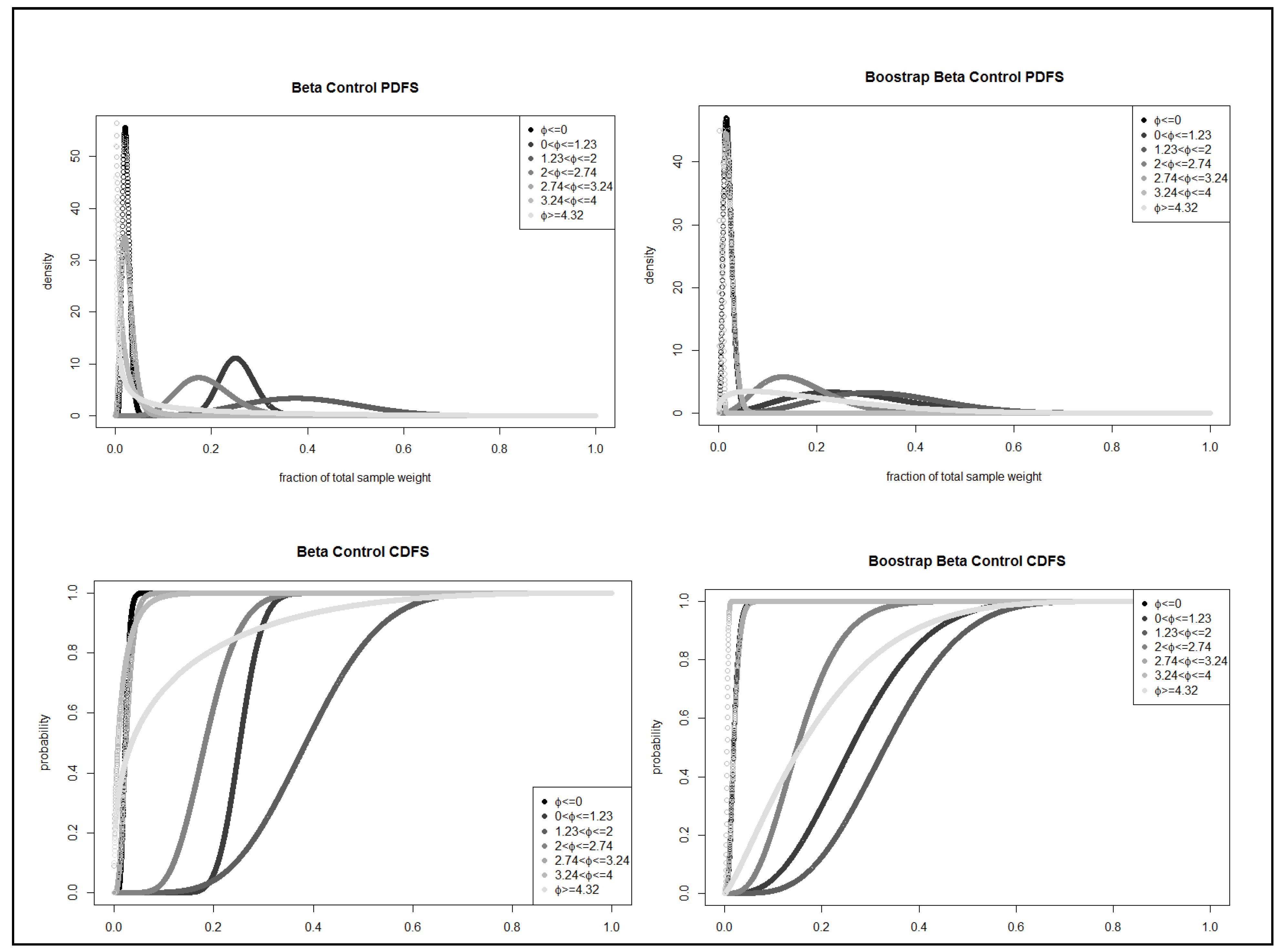
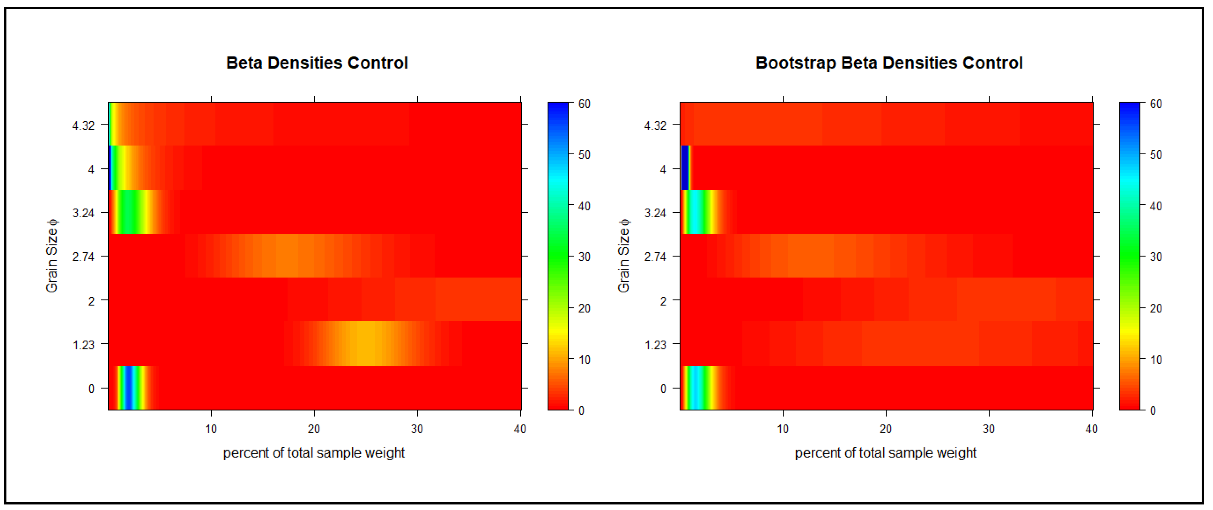
Figure 3 shows the PDF and CDF of the beta distribution for the original samples as well as the bootstrap sample of the control test. Heatmaps for the original samples as well as the bootstrap sample of the control test are depicted in
Figure 4. The fraction of the sample weight for small, relatively small, and very large grain sizes is almost zero (
Figure 3 and
Figure 4). The fraction of the sample weight for the very small and large grain size is up to 60%, while the fraction of the medium size and relatively large grain size is up to 30%. The fraction of the sample weight for the very small grain size is between 5% and 60%, for the medium size is between 10% and 30%, for the large size is between 20% and 60%, and for the relatively large size is between 20% and 30%. As demonstrated in
Figure 4, the medium, large, and relatively large sediment sizes made up more of the sample weight. Comparing this to the bootstrapped data, some similarities are observed. However, the densities of the data are less extreme, and the curves of the mid-range sediment sizes (medium, large, and relatively large) and the very small sediment size have stretched over a broader range. For example, the medium grain size was originally peaked somewhat steeply at around 25% of the total sample weight, while the tails of the curve asymptote to 0 at around 10–30%. However, comparing the same grain size of the bootstrapped data, the density peaks at around 15% of the total sample weight, while the tails span from 0% to around 35%. The PDFs for the same control test show that the very small or very large grain size will make up less of the sample, while the coarser size is more likely to make up a larger fraction of the sample. Similar results are interpreted from the bootstrap PDF. However, just as the bootstrap CDFs were stretched over the x-axis, the bootstrap PDFs are demonstrating a similar stretch over the x-axis. This shift means that of the bootstrapped data, the grain sizes are more likely to make up a larger range of the total sample. For example, the distribution of the original sample shows that the relatively large grain size has less than 10% probability of making up 20% of the total sample weight, while the bootstrap distribution data suggest a 30% chance of the relatively large grain size making up the same fraction of the sample (20% of the total sample weight).
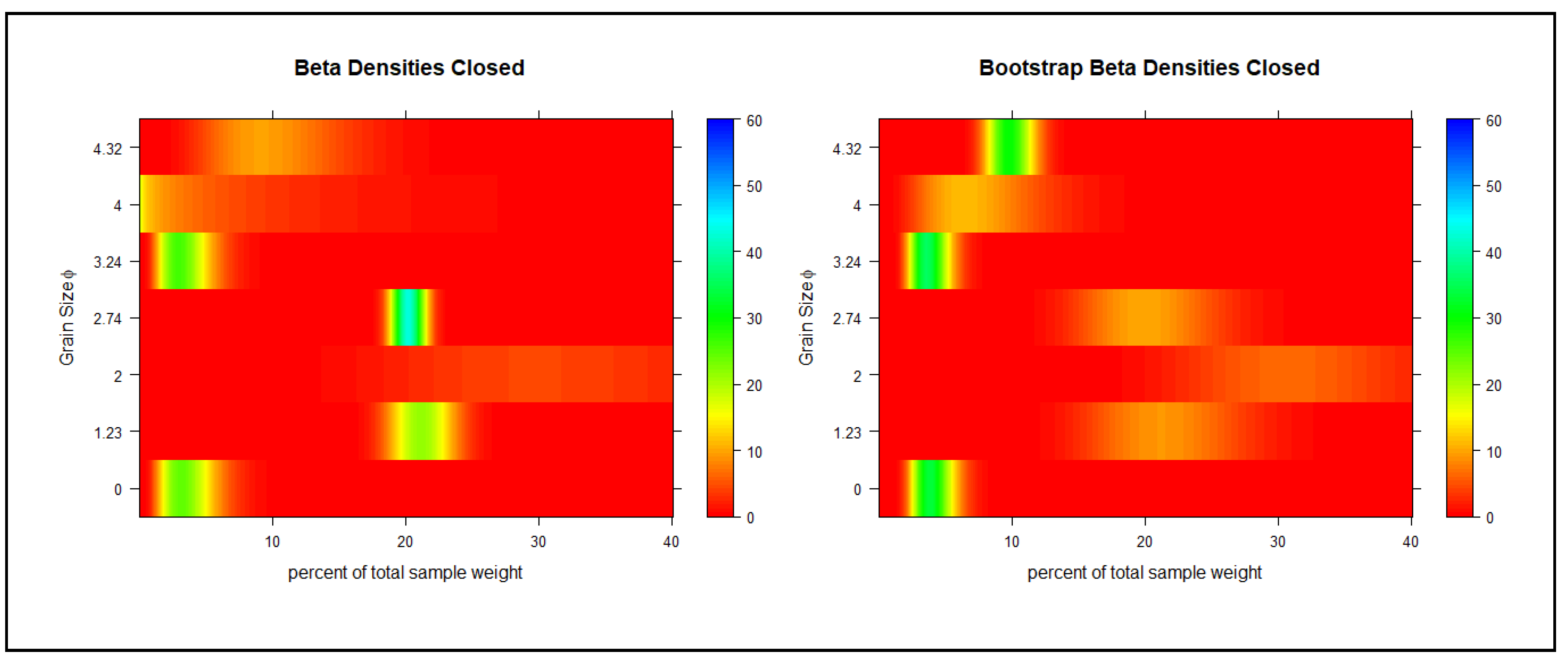
The results regarding the closed test exhibited much different results compared to the control group.
Figure 5 and
Figure 6 show the weight distribution for the closed setting. The distributions of the smaller grain sizes make up slightly more of the total sample weight in comparison with that of the control (close to zero). Similar to the control sample, the bootstrap distributions of the smaller gran sizes in the closed setting exhibited a spreading out along a larger fraction of the total sample weight. This can be seen more clearly in the comparison of the CDFs of the original sample and the bootstrapped one. For example, the distribution of the original sample shows that there is approximately a 20% chance that the relatively large grain size makes up 20% of the sample weight, while it is closer to 30% in the bootstrap distribution. Overall, looking at the distributions of the samples taken with the closed setting, the larger grain sizes were more likely to make up more of the sample weight. The smaller grain sizes also have a higher chance (although not likely) of making up slightly larger portions of the sample weights as compared to those of the control test. The results agree with the estimated log-normal distribution summarized in
Table 5, which shows that the closed test has a mean grain size much larger than that of the control test.
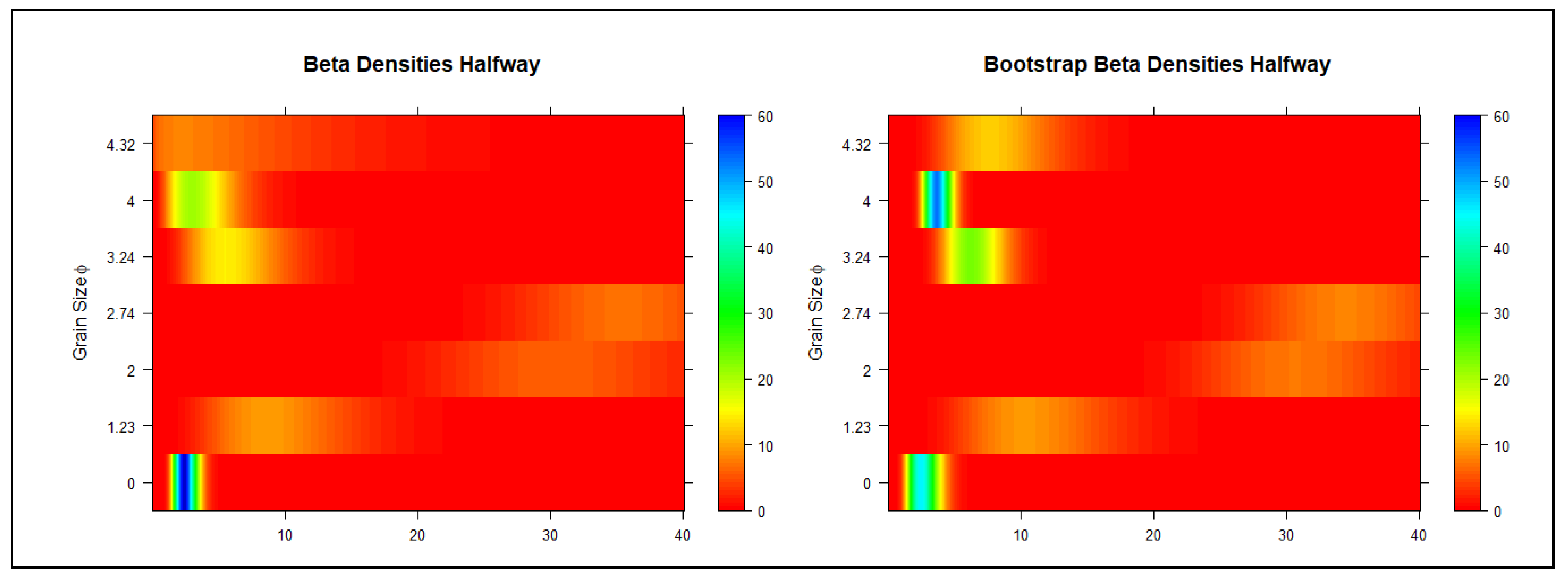
Moving on to the halfway test (
Figure 7 and
Figure 8), the differences in the distributions are more visible in comparison with both the control and closed settings. In the halfway setting, the distribution of the largest (very large) grain size shows that it is more likely (40%) not to pick up this grain size at all (1% of the sample weight) in comparison with the previous settings. This probability was closer to 30% and 20% for the closed and the control settings, respectively. As shown in the CDFs and heatmaps, the bootstrap distributions spread out more evenly over a longer range of sample weight. Moreover, there is a spike in the intensity for the largest grain size (
Figure 8, bottom row), which is indicated by the dark blue bar in the original sample and the light blue bar in the bootstrap sample.
Although the intensity of the bootstrap spike is reduced in comparison with the intensity of the original sample for the very large grain size, it has a slightly broader spread. In contrast, a bootstrap spike can be observed for the relatively small grain size, which does not appear in the heatmap of the original sample.
Finally, looking at the open setting,
Figure 9 and
Figure 10 show much different results compared to what was observed for the other test settings. The probability of not picking up the very large grain size (weight percentage close to zero) is about 50% in this setting, as there is a 50% chance (CDF in
Figure 9) that the very large grain size makes up just over 0% of the total sample weight. The bootstrap distributions are comparatively similar to the distributions of the original samples, but they spread out over a broader range of sample weight. The difference is substantial for the medium grain size depicted in
Figure 9 and
Figure 10. From the heatmap, it is noted that the medium grain size has a sharper intensity over a shorter length, while the bootstrap distribution has a dimmer intensity over a longer range. This difference for the medium grain size can be observed as a shift in the CDF from an impulse at about 40% of the total sample weight to a smoother increase between 30% and 45% of the sample weight in the bootstrap distribution. The differences between the distributions of the original and the bootstrap samples are more clearly illustrated in
Figure 10. For instance, the spike intensity peak for the very large grain size is shifted slightly to the right in the bootstrap, representing a larger fraction of the sample weight.
Reviewing the heat maps in
Figure 4,
Figure 6,
Figure 8, and
Figure 10 suggest that in almost all settings, the intensities of the smaller grain sizes, including small, relatively small, and very small (except for the very small grain size in the control test), become steeper. Moreover, the peak of the medium grain size is typically associated with a larger percentage of the total sample weight, and its bootstrap distribution is somewhat stretched in comparison with the distribution of the original samples in all settings except for the halfway test. In comparison with the distribution of the original samples, the bootstrap distribution of the large grain size is steepened except for in the control test. In comparison with the other grain sizes though, the distribution peak is substantially lower, and the distribution is spread across a broader range of sample weight. This demonstrates that there is more fluctuation on how much of the sample weight will be made up of a large grain size. Meanwhile, the bootstrap distribution of the relatively large grain size is flattened in all tests except for the open setting. Similarly, the bootstrap distribution of the very large grain size is flattened in all settings except for the open setting.
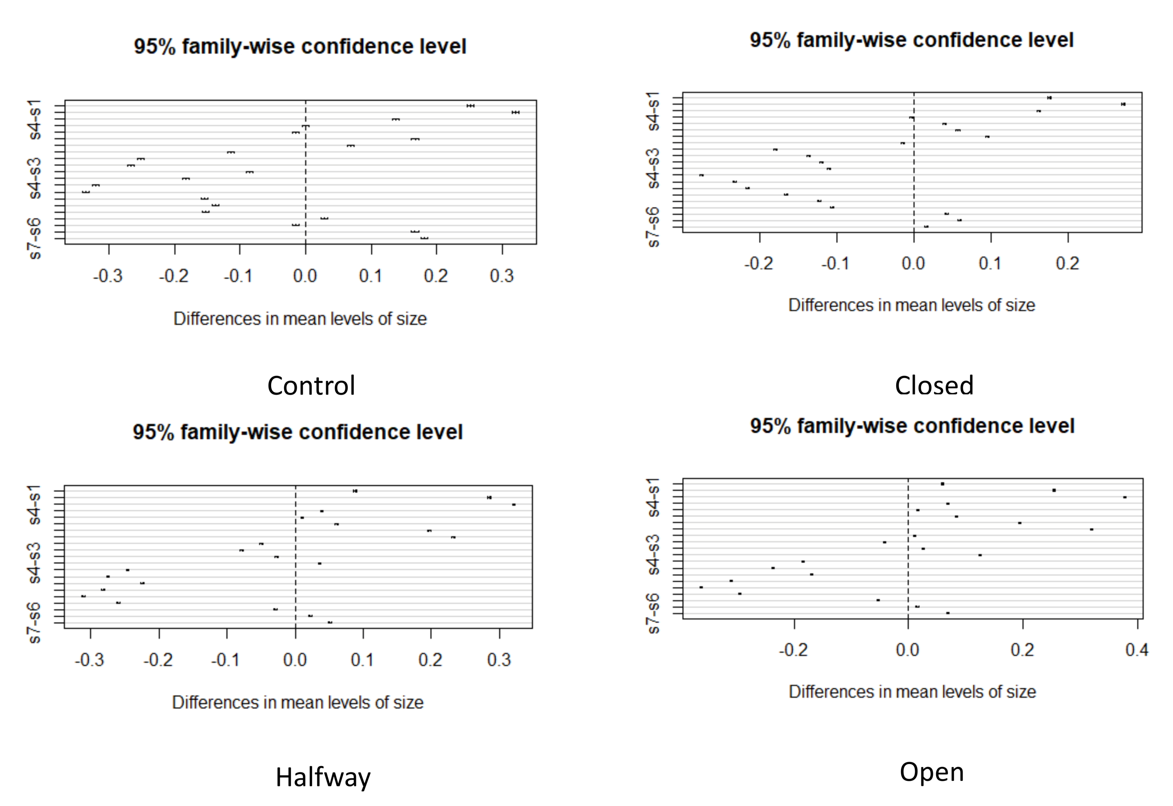
We also visualized the weight distribution for different grain sizes using the boxplot. Results are depicted in
Figure 11. By visual inspection, we can notice the difference in the mean weight for different grain sizes in all settings, including control, closed, halfway, and open. To investigate the statistical significance of mean weight differences for the different grain sizes, we used Tukey’s ‘Honest Significant Difference’ method. In this way, a set of confidence intervals were constructed for the differences between the means of different grain sizes with the specified family-wise probability of coverage where the intervals are based on the studentized range statistic. As we can observe in
Figure 12, no confidence interval contains zero, rejecting the null hypothesis that any given pair of grain sizes have the same mean weight. Lower bound, upper bound, and p-value for all confidence intervals for the different settings are reported in four tables in the
Supplementary Materials. Careful interpretation of the heatmaps and Tukey’s confidence intervals suggests significant differences in the weight proportion of each grain size. We must point out that while heat maps visualize the weight percentage of each grain size, Tukey’s confidence intervals demonstrate the difference in the mean weight percentages of the different grain sizes.


