Article

Improvements in Sub-Catchment Fractional Snowpack and Snowmelt Parameterizations and Hydrologic Modeling for Climate Change Assessments in the Western Himalayas

by
Vishal Singh
1 and
Francisco Muñoz-Arriola
2,3,*
1
Water Resources System Division, National Institute of Hydrology Roorkee, Roorkee 247667, India
2
Department of Biological Systems Engineering, University of Nebraska-Lincoln, Lincoln, NE 68583, USA
3
School of Natural Resources, University of Nebraska-Lincoln, Lincoln, NE 68583, USA
*
Author to whom correspondence should be addressed.
Hydrology 2021, 8(4), 179; https://doi.org/10.3390/hydrology8040179
Submission received: 5 November 2021 / Revised: 23 November 2021 / Accepted: 29 November 2021 / Published: 7 December 2021
(This article belongs to the Section Hydrology–Climate Interactions)

Abstract

:
The present work proposes to improve estimates of snowpack and snowmelt and their assessment in the steep Himalayan ranges at the sub-catchment scale. Temporal variability of streamflow and the associated distribution of accumulated snow in catchments with glacier presence in the Himalayas illustrates how changes in snowpack and snowmelt can affect the water supply for local water management. The primary objective of this study is to assess the role of elevation, temperature lapse rate (TLR), and precipitation lapse rate (PLR) in the computation of snowpack (or snowfall) and snowmelt in sub-catchments of the Satluj River basin. Modeling of snowpack and snowmelt was constructed using the Soil Water Assessment Tool (SWAT) in both historical (1991–2008) and near-time scenarios (2011–2030) by implementing real-time hydrometeorological, snow-hydrological parameters, and Global Circulation Model (GCM) datasets. The modeled snowmelt-induced streamflow showed a good agreement with the observed streamflow (~60%), calibrated and validated at three gauges. A Sequential Uncertainty Parameter Fitting (SUFI2) method (SUFI2) resulted that the curve number (CN2) was found to be significantly sensitive during calibration. The snowmelt hydrological parameters such as snowmelt factor maximum (SMFMX) and snow coverage (SNO50COV) significantly affected objective functions, such as R2 and NSE, during the model optimization. For the validation of snowpack and snowmelt, the results have been contrasted with previous studies and found comparable. The computed snowpack and snowmelt were found highly variable over the Himalayan sub-catchments, as also reported by previous researchers. The magnitude of snowpack change consistently decreases across all the sub-catchments of the Satluj river catchment (varying between 4% and 42%). The highest percentage of changes in the snowpack was observed over high-elevation sub-catchments.

1. Introduction

Perennial streamflow in river basins in India such as Ganga, Indus, and Brahmaputra originate from the Himalayan glaciers. Thousands of glaciers in the Himalayan Mountainous valleys formed by large snowpacks represent the major sources of fresh water and energy reserves in India [1,2]. Many studies reported that the hydroclimatology of the Himalayan basins is changing due to climate change. The permanent snowpack (or snowfall) and the glaciers are reducing their masses, which leads to more snowmelt water in the streams [1,3,4]. As per the Intergovernmental Panel on Climate Change (IPCC), temperature increase is the main cause of precipitation alteration in the Himalayan regions [1,5]. Some of these changes can be reflected in the spatial distribution and temporal variability of rainfall and snowfall, which at the same time can drive streamflow generation in large catchments in the Himalayas [6,7,8]. While snowpack and glaciers influence streamflow in high altitudes, rainfall is considered a predominant factor at low altitudes. As a main tributary of the Indus River, the Satluj river has its flow primarily generated by snowmelt during the spring. Thus, a higher measure of melting will result in an increase in runoff downstream before the monsoon season [9,10]. As in other regions around the world, the shift in runoff generation regimes may increase flood risk, affecting food, energy, and urban security downstream of the catchment areas [11,12,13,14].
Ref. [1,2] reported that the length of many Himalayan glaciers is shortening, and only 25% of glaciers are stable. Other areas of the world, such as the western United States of America, have experienced incremental increases at the altitude of snow accumulation reduction in the snowpack, and earlier snowmelt onsets due to climate change [8,15,16,17]. The glacier retreating and snowmelt variations due to climate change may influence water supply and storage and will affect the sustainability of human activities [18]; however, in the Satluj Sutlej River or Sutlej catchment, recent and projected changes in snowmelt and snowpack are inconclusive regarding about how glacial and perennial streamflow will be affected in a changing climate. As per the studies conducted by [8,19,20], the elevation-based fluctuations in temperature may affect the snowmelt process, especially over Himalayan regions. A few studies highlighted elevation-dependent changes in temperature and precipitation, especially in the high Himalayas [21,22]. Ref. [23] Elevation-dependent changes in air temperature over glaciers in Arctic regions revealed a significant variation in temperature lapse rate (TLR) and precipitation lapse rate (PLR). The variability in TLR and PLR can be the major cause of reduction in the snowpack at high elevations of the Himalayas [24,25,26]. The TLR and PLR are defined as the function of elevation [23], and thus the snowpack and snowmelt rate can be influenced significantly due to changes in TLR and PLR [19].
The ability of any hydrological model to simulate snowmelt runoff depends on how well the model performs for the snowmelt processes. The temperature index model and degree-day are factors widely assessed in snowmelt runoff diagnostics [9,20,27]. In the simulation of the temperature index, the decrease in snow water equivalent (SWE) or the amount of snowmelt is computed using a snowmelt factor and mean surface air temperature [27]. This snowmelt factor or degree-day factor drives the snow–glacier melt process since it is subject to changes in temperature. The temperature is dependent on the elevation affecting the degree-day significantly, as has been evidenced in Himalayan catchments by [20]. Previous researchers have used a constant degree-day factor for the whole domain of research, whereas the degree-day factor varies spatially as well as temporally. Thus, the role of elevation bands must be addressed in the computation of snowmelt and snowpack, which becomes relevant over catchments along with the Himalayan Mountain ranges.
The Global Circulation Models (GCMs) based studies revealed the impact of climate change on the variability of precipitation over the Himalayas [21,22,28]. Climate change is influencing TLRs and PLRs [21], particularly when catchments’ topography corresponds with moderate to very high elevations such as the Himalayas. Thus, snowpack and snowmelt amounts can be affected significantly in the high Himalayas. Further, the influences of a changing climate in the Himalayan region have evidenced long-term shifts in average air temperature, precipitation, and other land surface variables [9,29,30,31]; therefore, future changes, especially near-term changes, have made it increasingly important to be able to compute snowpack and snowmelt in sub-catchments to manage water resources.
The focus of this study is to assess the role of elevation bands coupled with SWAT based temperature index model [27] in the computation of snowpack and snowmelt over Himalayan catchments. Another objective of this study is to analyze the role of model parameters in snowmelt modeling to reduce parameter-related uncertainties, which would help construct more accurate snowmelt models at the sub-catchment scale. The sensitivity analysis of modeling parameters was performed to identify the behavior of snowmelt and other water balance parameters. Studies revealed the importance of sensitivity analysis in hydrological modeling [32,33,34]. The Nash–Sutcliffe Equation (NSE) and coefficient of determination (R2) [35] are used as the main objective functions. The third objective of this study is to highlight the snowmelt and snowpack changes and their comparisons with the previous studies in the historical and near-term time scenarios. No previous study accounted for a fractional variability assessment of snowpack and snowmelt at each sub-catchment scale over Himalayan catchments. In this study, the two most influencing climate factors, daily minimum–maximum temperature and daily precipitation, have been emphasized to highlight the changes in a glacial Himalayan catchment. The TLR, PLR, and other snowmelt parameters (e.g., seasonal degree-day factors) are optimized using a Sequential Uncertainty Parameter Fitting (SUFI2) utilizing observed snowmelt induced streamflow at three gauge locations. SWAT has already proven its capability in the computation of snowpack and snowmelt [27,33,36].

2. Materials and Methods

2.1. Study Area

For the present study, the Satluj river catchment (up to Kasol gauge station) was selected. The Satluj river flows through the western Himalayan region and is a part of the Indus River basin. The Indus River has many major tributaries, such as the Satluj, Beas, Jhelum, Chenab, Ravi, and minor tributaries. The main outlet station of the selected study area, such as Kasol, consists of an area of about 51,055 km2, which is located at the head of the Bhakra dam of India. The geographical extent of the study area lies between 77°00′ to 82°39′ E longitudes and 30°8′ to 33°00′ N latitudes (Figure 1). The Satluj river is the longest river among the five major rivers that flow through northern India and Pakistan. It is north of the Vindhya Range, south of the Hindu Kush segment of the Himalayas, and east of the Central Sulaiman Range in Pakistan. The Satluj catchment is mainly covered by snow and glaciers, which cover around 61% of the total catchment area as classified in the land use/land cover (LULC) map. The Satluj river catchment corresponded to around 10.21% of the total Indian Himalayan region [9]. The Satluj river catchment elevation varies from moderate (526 m) to very high elevations (7429 m). The majority of the Satluj river catchment is fed by snowmelt (up to the Rampur gauge station) and rainfall during the summer and by groundwater flow during the winter.

2.2. Meteorological and Thematic Data

For the research work, we used the observed gridded (at 1° × 1° scale) daily precipitation and daily minimum and maximum temperatures (1989–2008) obtained from the Indian Meteorological Department (IMD) and Indian Institute of Tropical Meteorology (IITM). A total of 8 grids covering the catchment area were selected (Figure 1). These datasets were generated using more than 1800 observed precipitation and temperature gauges distributed across India. These gridded precipitation and temperature datasets were increasingly used in studies on the Indian and Himalayan continents [21]. Additionally, the measured gauge-based daily precipitation datasets for the same year 1989 to 2008 were available at the three gauges at Rampur, Suni, and Kasol, which were utilized for the analysis. The historical simulation (1991–2008) of snowpack, snowmelt, and other water balance components was generated using these gridded hydrometeorological datasets. The initial two years (1989–1990) are taken as the warmup period. For the historical model simulation (1991–2008), the observed temperature and precipitation gridded datasets were spatially adjusted at each sub-catchment scale utilizing the TLR and PLR [21]. The whole basin was categorized into 16 sub-catchments based on the default threshold area [33,37].
Each grid point has been spatially adjusted at the centroid of each sub-catchment, and accordingly, the precipitation and temperature have been adjusted. For the adjustment of the meteorological variables, the average TLR and PLR have been computed to highlight the effect of elevation variations across the sub-catchments [21,33]. The spatial adjustment of each grid point at the centroid location of the sub-catchments enhances the local climatological effect in the snowmelt computation [21]. The methodology of TLR and PLR is explained in Section 2.5.1. Snow and glaciers mainly cover the upper part of the catchment that has a very low TLR, while the lower part of the catchment has a reduced presence of glacier areas with large settlements and high temperatures. These topographical variations brought high variability in TLR and PLR over the Satluj river catchment, and thus, snow cover could be sensitive to the temperature variations [21]; therefore, ten elevation bands were computed at each catchment scale to account for the effect of temperature in the snowpack.
The Shuttle Radar Topographic Mission (SRTM) digital elevation model (DEM) with 90 m spatial resolution [38] was used to delineate the catchment boundaries, stream channels, flow paths, fractional slopes, and elevation bands. The SRTM DEM was downloaded freely from NASA’s earth explorer portal (https://earthexplorer.usgs.gov/ 12 June 2021). The thematic data layer such as land use/land cover (LULC) map prepared at 1:50,000 topographical scale using Indian Remote Sensing satellite (IRSP6) Linear Imaging Spectral Scanner (LISS) III satellite images (https://bhuvan-app3.nrsc.gov.in/data/download/index.php 12 June 2021). The LULC maps were reclassified based on the SWAT manual [37]. The soil map of the study area was downloaded from SWAT’s portal (http://swat.tamu.edu/data/india-dataset/ 12 June 2021) [39]. The description of soil categories was provided in the FAO’s world harmonic soil database [39] (Figure 1). The LULC and soil categories for the Satluj catchment are shown in Figure S1. The Satluj river catchment was discretized into 16 sub-catchments. Each sub-catchment includes a main channel and multiple Hydrological Response Units (HRUs), which consist of geospatial representations of homogeneous land use, soil type, and management practices.

2.3. GCM Datasets and Projection Scenarios

For the assessment of near-term (2011 to 2030) snowpack, snowmelt, and snowmelt induced water yield, the daily precipitation and temperature datasets were downloaded from the Intergovernmental Panel on Climate Change (IPCC) climate data portal. In this study, the Coupled Global Climate Model (CGCM3.1)/T63 atmospheric and sea-ice model output—namely, the SRES B2 model experiment [40,41]—was used to generate near-time scenarios. SRES GCM scenarios find significant changes for the near-term prediction and projection of watershed variables using temperature and precipitation datasets [40,41,42]. CMIP3 SRES B2 experiment-based daily temperature and precipitation datasets at 128 × 64 Gaussian grid (approximately 2.5° latitudes × 2.5° longitudes) are then downloaded. Four GCM data points, which are falling inside/near the current study area and highlight the spatial variations of the present study, are considered (Figure 1) without downscaling [43]. These four GCM grids have been spatially interpolated at each sub-catchment scale using the Inverse Distance Weighting (IDW) method [44,45]. For the GCM datasets, the statistical bias correction was performed with reference to the observed daily temperature and precipitation datasets [22,46]. This study did not perform the GCM data uncertainty. However, to preserve the local scale effect of GCM variables (e.g., temperature and precipitation), the mean bias was computed at each sub-catchment scale, and accordingly, the GCM variables were corrected.
The SRES B2 scenario emphasizes local rather than global solutions to economic, social, and environmental stability and thus was found to be more reliable for the near-term assessment [41,47]. The SRES B2 experiment was referred to by various researchers in various climate change studies around the world [40,41,44,46,47] and hence was used in this study. The SRES B2 model experiment was finally selected for the near-term assessment based on the comparison of IPCC’s SRES B1, SRES A2, 20C3M, COMMIT, and B2 historical simulations and observed precipitation and temperature [47]. Finally, the bias-corrected GCM variables, such as daily temperature and daily precipitation, were then incorporated into SWAT to generate the near-term scenarios. During the computation of near-term scenarios, the GCM-based temperature and precipitation datasets were taken as the variable parameters and other parameters were kept constant. The optimized coefficients and parameter values were again incorporated into SWAT and then the near-term scenarios of snowpack and snowmelt were generated. It is noteworthy to mention that the use of CMIP-based scenarios represents a viable alternative to test the proposed methodology and, at the same time, provided a diagnosis of the impacts of climate change on snowpack simulation and scenarios.

2.4. Modeling Approach

The SWAT model is fully capable of computing the long-term water balance components in a semi-distributed manner using hydrological response units (HRUs) (Arnold et al. 1998). The Satluj river catchment was divided into 16 sub-catchments and 358 HRUs based on the unique combination of soil, LULC, and slope. The water balance components were computed at each HRU scale, and then their aggregation was determined at each sub-catchment scale [27,32,48]. The rationale for discretizing the catchment is to simulate streamflow, snowfall, and snowmelt at the sub-catchment scale. The representation of snowpack and snowmelt at each sub-catchment by the function of multiple elevation bands could be useful to highlight their variabilities in an efficient manner, especially in the case of topographically variable catchments. In this study, the Soil Conservation Services (SCS)-based curve number (CN) method was used for the water balance computation. The CN is a function of LULC, various soil conditions, and antecedent moisture conditions (AMCs), which includes around 150 different parameters, including snowmelt parameters [37,48]. The Satluj river catchment corresponded to steep slopes and has a very complex topography; therefore, to account for the effect of steep slopes in the overall water balance computation, we employed a slope-adjusted modified CN method for the computation of water balance components [37]. The CNs were modified as per the fractional slopes computed at each HRU scale, which enhanced the accuracy of the simulated streamflow [37].
The main hydrological processes included interception, infiltration, runoff, evapotranspiration, lateral flow, and percolation. The details about the physical and hydrological principles and parameters of SWAT are fully described in the SWAT user manual [37]. In this study, the linear reservoir approach was applied for the computation of snowpack and snowmelt by the fractional computation of snowpack and snowmelt [28]. The aggregated snowpack and snowmelt amount with respect to multiple elevation bands accounted for at each sub-catchment scale [37]. For each sub-catchment, a maximum 10 elevation bands are constructed. The five basic snowmelt parameters such as degree day melt factor maximum (4.5 mm/d/°C), degree-day melt factor minimum (2.5 mm/°C/d), snowfall temperature (0.0 °C), snowmelt temperature (0.5 °C), and snow water content for 100% snow cover (100 mm) were incorporated in SWAT with their standard global values during default simulation [37]. Since very limited studies were performed with respect to snowmelt and glacier hydrology over the western Himalayan regions, thus, the regional/global values were adopted as per their availability for model simulation [28,37]. In this study, the snowmelt parameters are considered as the model calibration parameters.

2.5. Elevation Band Approach for Snowpack and Snowmelt Measurement

In this study, the temperature index model was constructed to compute the snowpack and snowmelt (Fontaine et al., 2002). The seasonal degree-day melt factors (e.g., maximum and minimum) with their global coefficient values obtained from the literature survey are employed in the model for the computation of snowmelt [20,27,28,49]. In the Himalayan region, the degree-day melt factor varies from 1.5 mm/°C/d to 4.7 mm/°C/d [20,27]. Initially, [28] developed the methodology for the snowmelt module and showed that the elevation band-wise characterization of snowpack and snowmelt significantly enhanced. Thus, each sub-catchment was categorized into a maximum of 10 elevation bands to improve the simulation of snowpack and snowmelt. The elevation bands were defined based on their mean elevation and the proportion of the sub-catchment area they encompass. To incorporate the temperature and precipitation variations across the sub-catchments, the TLR and PLR were computed and adjusted with respect to the altitude of the corresponding sub-catchment [37]. The sequence of methodological steps are as follows:

2.5.1. TLR and PLR Computation and Their Adjustments at Each Elevation Band

For each sub-catchment, lapse rates for precipitation plaps (mm/km) and temperature tlaps (°C/km) were computed as Equations (1) and (2), respectively:
P B = P + ( Z B Z ) p l a p s days p c p , y r × 1000
T B = T + (   Z B Z ) t l a p s 1000
where P (mm), T (°C), and Z (m) were the sub-catchment precipitation, temperature, and recording gauge elevation, respectively, while PB, TB, and ZB were the adjusted precipitation, temperature, and mean elevation for each elevation band. The variable daypcp,yr represented the mean annual number of days with precipitation. The TLR could be computed using mean annual temperature. In accordance with the delineation approach used with sub-catchments, temperatures were adjusted within each elevation band by comparing the elevation bands’ midpoint elevation (ZB) within the station elevation (Z). The elevation difference was multiplied by the lapse rate to calculate a temperature difference between the station elevation and the elevation band. An updated elevation band mean temperature (TB) was calculated by adding or subtracting the temperature difference to or from the temperature measured at the station elevation (T) as in Equation (3):
T B = T + ( Z B Z ) dT dZ
where dT dZ is the mean local lapse rate ( t l a p s ) (°C/km) calculated at all sub-catchments. A lapse rate for annual precipitation was represented by the changes of the mean annual precipitation with respect to the station elevation. Adjusted precipitation in each elevation band (PB) was based on the difference between the elevations of the sub-catchment meteorological station (Z), and each elevation band (ZB) multiplied by the lapse rate of (mm/km) per event (P). If the meteorological station was unavailable in a particular sub-catchment, then the next nearest meteorological station was considered for lapse rate calculations. The equation was defined as Equation (4):
P B = P + ( Z B Z ) dP dZ
where d P d Z was the mean local lapse rate   ( p l a p s ) calculated for all sub-catchments.

2.5.2. Snow Accumulation

SWAT differentiates snowpack (solid precipitation) and rainfall (liquid precipitation) based on near-surface daily air temperature. The snowpack (depth) was represented in SWAT by the snow water equivalent (the mass of liquid water in the snowpack) SWE (mm), which balanced snowfall SF (mm) and snowmelt SM (mm) or sublimation ES (mm) (Equation (5)):
SWE d a y = SWE ( d a y 1 ) + SF SM E s
In SWAT, SM is controlled by the air and snowpack temperatures, the melting rate, and the areal coverage of snow. When the daily mean air temperature is less than a snowfall temperature, as specified by the SWAT variable SFTMP (Table 1), the precipitation within an HRU is classified as snow, and the liquid water equivalent is added to the already-present snowpack. The snowpack temperature is a function of the mean daily temperature during the preceding days and varies as a dampened function of air temperature [49]. The influence of the previous day’s snowpack temperature on the current day’s snowpack temperature was controlled by a lagging factor, (TIMP), which intrinsically accounts for snowpack density, snowpack depth, exposure, and other factors known to affect snowpack temperature (Equation (6)):
T s n o w p a c k ( d a y ) = T s n o w p a c k ( d a y 1 ) × ( 1 TIMP ) + T a v TIMP
where Tsnowpack (day) and Tsnowpack (day−1) are the snowpack temperature (°C) on a given day and on the day preceding it, respectively, and Tav (°C) is the mean air temperature for the same given day. The fraction of area covered by snow SNOcov can be computed as Equation (7):
snow c o v = SNO SNO 100 ( SNO SNO 100 + exp ( cov 1 cov 2 SNO SNO 100 ) ) 1
where SNO is the water content of the snowpack on a given day (mm), SNO100 is the threshold depth of snow at 100% coverage (mm), and cov1 and cov2 are coefficients that define the shape of the curve. Snow depth over an elevation band is assumed to be constant when the SWE exceeds SNO100; i.e., the areal depletion curve affects snowmelt only when the snowpack water content is between zero and SNO100. The SNO100 (e.g., the initial snow coverage) was computed using LISS3 satellite datasets. The values of cov1 and cov2 were adopted from the study carried out by [50].

2.5.3. Snowmelt and Glacier Melt

In the SWAT model, the snowmelt rate is controlled by snowpack temperature and air temperature. A snowpack cannot begin to melt and release water before the entire pack has reached 0 °C [27]. SWAT model provides melt water at each sub-catchment scale which includes the contribution of melt water from both snow and glaciers [37]. To incorporate the melt effect from the glacier area, the percentage of glacier area (20%) within the Satluj river has been incorporated [9]. The standard global coefficient related to glacier melting (e.g., glacier temperature) has been incorporated to account for melt release from glaciers, similarly applied by [51]. The melt rate from a snowpack/glacier varies in response to snowpack conditions [28]. In SWAT modeling, the snowmelt and glacier melt were set up together as a linear function of the differences between the average of the snowpack and glacier temperature (Tsnowpack), and the maximum air temperature (Tmax) on a given day and the base, or threshold temperature, for the snowmelt (Equation (8)); however, the SWAT model does not differentiate the melt water from glacier and non-glacier areas. The snowmelt (SM) can be computed as:
SM = b m l t × sno c o v [ T s n o w p a c k + T m e l t 2 TMLT ]
where bmlt (mmH2O/day-°C) in Equation (9) is the melt factor for a day:
b m l t = SMFMN + SMFMX 2 + SMFMN SMFMX 2 sin ( 2 π 365 ( d n 81 ) )
Equation (9) has been adapted for application in the Northern Hemisphere, where SMFMN is the melt factor for 21st June, SMFMX is the melt factor for 21st December, and dn represents the day of the year [37].

2.6. Model Calibration and Validation

The main aim of the calibration of snowmelt-induced streamflow is to produce more accurate water balance components; therefore, the observed snowmelt induced streamflow time-series datasets (1989 to 2008) at the three-gauge locations, such as Rampur, Suni, and Kasol (outlet point), obtained from the Central Water Commission (CWC) India, were used for the calibration and validation of modeled snowmelt induced streamflows. The accuracy and reliability of the modeled snowpack and streamflow depend on the overall water balance parameters and their optimized coefficient values. The model strength was evaluated using objective functions, such as coefficient of determination (R2) and Nash–Sutcliffe Equation (NSE) index [52]; however, we assume that the reasonable NSE and R2 results are not fully sufficient to judge the snowmelt modeling strength of a model that indicates how accurate (%) our model is for the computation of snowpack and snowmelt; therefore, the modeled outcomes, such as snowpack and snowmelt, are also validated/compared with the previous studies performed over the Satluj river catchment [9,20,53].
A deterministic-approach-based hydrological model such as SWAT is unable to explore the stochastic behavior of meteorological variables such as precipitation in the streamflow simulation [32,52]; thus, SWAT Calibration and Uncertainty Program (SWATCUP)-based Sequential Uncertainty Parameter Fitting method (SUFI2), an optimization algorithm, [52] was used to analyze the different model calibration parameters and uncertainty analysis. The model was calibrated and validated at both daily and monthly time scales. The main aim of the calibration is to reduce the model uncertainties, mainly through parameterization, to compute a more accurate estimation of water balance components at a smaller scale. The model calibration was performed based on the concept of aggregate parameter selection [54]. An ‘aggregate parameter’ was obtained by adding terms such as v, a, and r to the front of the original parameter to create an absolute increase and a relative change in the initial parameter values, respectively [55].

2.7. Parameter Uncertainty and Sensitivity Analysis

The main goal of the parameterization and sensitivity analysis is to improve the model simulation in historical and near-term projection scenarios, especially through GCMs. Thus, in near-term scenarios, the optimized parameters and coefficients have been used. The optimal values of model calibration parameters improve the overall model performance, and thus, more accurate water balance components can be generated. Model parameterization and sensitivity analysis using observed hydro-observation datasets always lead to non-identifiable parametric uncertainties, which may be expected with hydrological processes and datasets, especially in the case of the snow-glacier induced catchment [52,54].
SUFI2 accounts mostly for parameter uncertainty through a Latin hypercube sampling (LHS) method, which constructs a “stratified-random” sampling method unlikely to Monte Carlo simulation [52,56]. The resultant simulated variables and state variables are contrasted to the equivalent observations through the application of an objective function (e.g., NSE/R2) [32,56]. The SUFI2 algorithm assumes a large parameter uncertainty (or physically meaningful range) occurring in response to data inputs to ensure the observed data fall into the 95% prediction uncertainty (95PPU) band during the first iteration [57]. During this iterative procedure, uncertainty progressive decrease is monitored through the changes of the p-factor and r-factor [32,52,56]. In each progressive iteration, the uncertainty band reduces, and we obtain a more concise parameter value. The p-factor determines the percentage of simulated data falling into the observed-data range, and the r-factor contributes to determining the uncertainty of the simulated variables and state variables when compared with observed datasets [56]. The value of the p-factor ranges between 0 and 100%, and the r-factor ranges between 0 and infinity. A value of p-factor = 1 and r-factor = 0 represents a perfect match between simulated and observed data.
In the SUFI2 algorithm, the old coefficient parameters (e.g., default parameter values) iteratively change and are updated into a new array of coefficients during calibration to ultimately achieve the final set of parameters. In this way, it improves the parameter coefficient values and reduces the parameter uncertainty. In this study, each iteration contained around 600 simulations to analyze the uncertain effect of model parameters. In this study, we ran four iterations to obtain the best-fitted coefficients and parameter values during both daily and monthly calibrations. Correspondingly, we performed the sensitivity analysis to identify the most model influencing parameter. It helps to identify the significance of a particular parameter to the calibration process, whether the process is influenced by the parameter values or nature of the forcing. In this study, we performed a global sensitivity analysis (GSA) through multiple regressions.
In sensitivity analysis, the statistical significance tests such as p-value and t-stat are employed to rank parameters from highly sensitive to non-sensitive. The p-values closer to zero will enable the use of trend analyses of the simulated variables and state variables [56]. The parameter value towards zero will be more significant. The GSA was evaluated based on the significance level alpha (α = 0.05). The alpha value 0.05 was chosen as the local significance level [56]. Based on this significance level, values larger than +1.96 indicate a significant (p < 0.05) positive sensitivity of the parameter, and values lower than −1.96 indicate a significant negative sensitivity. The model simulation details are given in Table 1 and parameter details are given in Table S1.

3. Results

The thematic components, such as topography, LULC, and soil classes, are parameterized in SWAT [37]. For example, more than 30 different soil parameters associated with each soil category, such as soil texture, available water content, hydraulic conductivity, bulk density, and organic carbon content, were used to setup SWAT simulation. These parameters in SWAT were defined for each soil subtype for different layers (between two and three layers). The average curve number (CN) (average of all HRUs) has been computed around 80 in the catchment, though it varied from lower sub-catchment to upstream sub-catchment as per the unique combination of LULC, slope, and soil. SWAT information on model implementation, including the temporal context for the simulated water balance components, is described in Table 1. The model calibration, parameterization, and sensitivity results were a product of 20 different hydrological parameters (Table S1) on both daily and monthly time steps. In Table S1, the parameters that were relevant to snowmelt-induced streamflows are selected for model parameter selection and calibration, and sensitivity analysis. The description of parameters and their coefficients are given in Table S1. The optimized best-fitted parameter values and their statistics of sensitivity on both a daily and monthly basis are shown in Table S2. Further, Table S2 shows the aggregate parameter ranges that result from the final iteration number optimized through the Latin Hypercube Sampling (LHS) method [56].
Table 2 and Figure 2 show the daily and monthly results for streamflow calibration (1991 to 2000) and validation (2001 to 2008) at all three outlet locations, Rampur, Suni, and Kasol. Figure 3 shows the sub-catchment-wise snowpack and snowmelt with reference to precipitation. Figure 2 shows the regression plots between the observed and calibrated/validated streamflows at all three gauges. The plotted regression lines showed an optimal correlation between observed and calibrated/validated snowmelt-induced discharge. Table 2 shows the goodness-of-fit between the calibrated/validated and measured streamflows with the R2 and NSE at all three gauges, such as Rampur, Suni, and Kasol (outlet) gauges. The computed R2 and NSE are found reasonably acceptable for daily and monthly observations (Table 2 and Figure 2). Regarding goodness-of-fit aspects, monthly and daily calibration correlations were similar. Among all the three outlet gauges, Kasol and Rampur show slightly better calibration and validation statistics than the Suni station. Yet, the consistency of the efficiency statistics also indicates consistency in the performance of the model. Before the initialization of the model calibration, we took 5% as a bias to ignore the extreme ambiguities from the calibration. The overall R2 and NSE between the computed and observed snowmelt induced discharge are computed ~0.7 and ~0.6, respectively.
The calibration process includes surface, groundwater, and snowmelt hydrology parameters. The focus was to calibrate snow hydrology parameters. Among twenty calibration parameters, five parameters such as R_CN2.mgt, R_SMFMX.bsn, V_CH_K2.rte, TLAPS.sub, and V_GW_DELAY were found significantly sensitive for daily calibration, while four parameters such as SNO50COV.bsn, CN2.mgt, GW_DELAY.gw, and SOL_K.sol were found significantly sensitive for a monthly calibration. For example, the TLAPS.sub parameter shows variation in the daily temperature at each sub-catchment scale. The parameter range for TLAPS.sub (or TLR) fluctuated from −7.0 °C/km to 2.5 °C/km and the best-fitted value was computed as −4.1 °C/km. This highlights the sensitivity of temperature variations across the Satluj river sub-catchments. For TLAPS.sub, the p-value is recorded as 0.01, and its t-stat value is recorded as −2.2, which is found to be significantly sensitive for the model calibration. The TLR is defined as the function of elevation. It clarifies the existed variations in snowpack and snowmelt amount across the elevation bands and catchments.
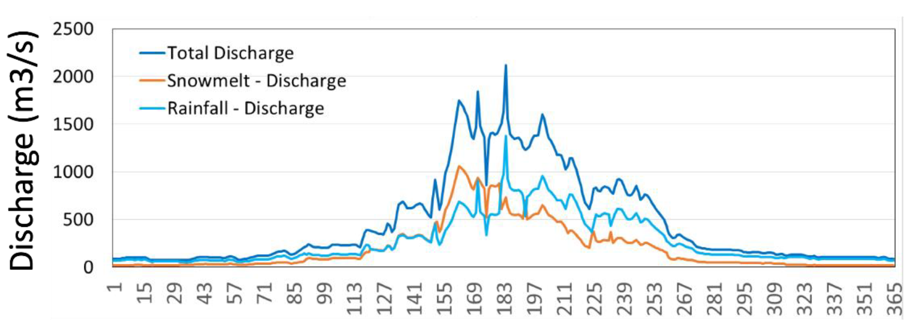
For the validation of snowmelt and snowpack modeled from the temperature index model by the aggregation of elevation bands, we referred to previous studies in the similar study area of Satluj River [9,20,53]. Figure 3 shows the daily averaged discrimination of snowmelt-induced streamflow and rainfall-induced streamflow. As per Figure 3, the snowmelt is maximally accounted for during May and June (~60% of total flow), while in July, it shows less than rainfall-induced streamflow due to the monsoon effect. The validation/comparative statistics of snowpack and snowmelt between modeled and reference values are shown in Table 3. Table 3 highlights a good agreement between the modeled data and referenced data from previous studies. The majority of the studies reported snowmelt contribution to the annual runoff is around 60%. The overall outcomes of this study are comparable to previous studies [9,20,53].
The sensitivity of TLR (TLAPS.sub) variations clearly shows that the elevation differences significantly affected the distribution of snowpack and snowmelt across the whole catchment. The Satluj river catchment is dominated by temporary/permanent snow covers, glaciers, permanent ice sheets, and seasonal well-packed snow. They are typical features of the catchment, which, at the same time, are identified in the sensitivity of parameters. The parameters such as SNOCOVMX.bsn and SNO50COV.bsn (parameters that represent the fraction of snowpack and the elevation bands) have been found to be significantly sensitive (Table S2). They computed t-stat values less than −2.2 or greater than +2.2, and their estimated p-values were close to zero. These parameters show that the snow depletion curve has a significant influence on the snowmelt process. Thus, the seasonal variations in the snowmelt factor could be sensitive for snowmelt and glacier melt rates. As in other latitudes, soil properties also evidence the regulatory role of infiltration in the subsurface [57]. For example, the V_GW_DELAY.gw parameter of aquifer recharge at the catchment was found to be significantly sensitive for both daily and monthly time steps (Table S2). In unconfined and shallow aquifers, this factor could influence the temporal variability and spatial distribution of different components of the water balance, highlighting the contributions of surface water and groundwater interactions. Further, at the catchment scale, A_ALFA_BF.gw, whose p-value was recorded as 0.2 daily and 0.4 monthly, were found insignificant for the model calibration. This evidence indicates that the model grapples with capturing possible surface water–groundwater interactions and the associated discharge–recharge rates, which can also be seen in data-driven models [58].
Other model parameters associated with different types of LULC and soil categories were not considered sensitive for the model calibration and validation process. These model parameters included GWQMN.gw, HRU_SLP.hru, SOL_BD.sol, PLAPS.sub, CH_N2.rte, SOL_AWC.sol, and GW_REVAP. The snowmelt temperature-related parameters, such as R_SMTMP.bsn, R_SFTMP.bsn, and R_SMTMP.bsn, were recorded as non-significant during model calibration, as shown in Table S2. These properties are relevant to the temperatures that allow the formation or accumulation of snow, rather than the melting of snow already packed (which coincides with the sensitivity of the SMFMX parameter described above). They were not recognized as significantly sensitive because their computation was less uncertain. The curve number coefficient (R_CN2) was found most to be the significantly sensitive parameter in the model calibration process. The CN varies for each HRU; therefore, the CNs were modified based on the fractional HRU slopes and calibrated at each HRU scale. The LULC and soil physical properties vary at the HRU scale. This makes the snowmelt-induced streamflow calibration more effective at smaller scales. The groundwater delays and baseflow, together with management practices, soil physical properties, and snow properties, influence the generation of return flows, which aligns with the purpose of this work in the Satluj river catchment.
Each parameter transports several uncertainties in the calibration process; therefore, the stochastic calibration process using SUFI2 was found helpful to minimize the uncertain effects of the parameters listed above. The uncertainty results were computed using two objective functions, such as p-factor and r-factor (Table 2). The results provide insights into the precision and accuracy of model calibration and their simulations. Further, they refer to the final uncertainty levels of the calibration-validation approach. The p-factor values were recorded as 0.46, 0.57, and 0.52 on a daily time step and 0.41, 0.57, and 0.49 on a monthly time step during model calibration for Rampur, Kasol, and Suni stations (1991–2000) (Table 2). During model validation, the p-factor values were recorded as 0.43, 0.52, and 0.53 on a daily time step and 0.45, 0.60, and 0.58 on the monthly time step, respectively. The p-factor values indicated that more than 50% of the simulated snowmelt-induced flows were encompassed within the uncertainty bonds for Kasol station on both daily and monthly calibration and validation, respectively. In contrast, simulated flows for Rampur showed p-factors below 50%, contrasting with their performance on the SWAT model for Kasol and Suni stations during daily simulations and for model validation, both downstream of Rampur.
On the other hand, the r-factor values were recorded as 1.89, 1.50, and 1.60 on a daily time step and 1.90, 1.57, and 1.43 on the monthly time step for Rampur, Kasol, and Suni. During model validation, the r-factor values were calculated as 1.89, 1.67, and 1.72 on the daily time step and 1.92, 1.62, and 1.52 on the monthly time step for Rampur, Kasol, and Suni, respectively. Resultant r-factor values indicated the SWAT’s ability to reproduce snowmelt induced flow values; however, values above 1.43 indicated that other sources of error besides model physics could contribute to the values of the r-factor. The experiments described here are unable to identify the contribution of such sources of error. Kasol, Suni, and Rampur were the only stations with observed data, and all were in the lowest drainage area in the Sutlej River catchment. The small differences among model performance metrics illustrate the local contributions of Suni and Rampur’s downstream drainage areas to the total streamflow generated at Kasol. Kasol averages over and under estimations of snowmelt-induced streamflows generated upstream, so lower r-factor values are expected, representing higher precision. Furthermore, the values of p-factor in Kasol in a daily time step (0.57) also indicate an average accuracy (~60%) of the model in replicating observed streamflows within the uncertainty bands. These results are acceptable as compared to previous studies, especially in the case of high uncertain snowmelt induced in the Himalayan catchment.
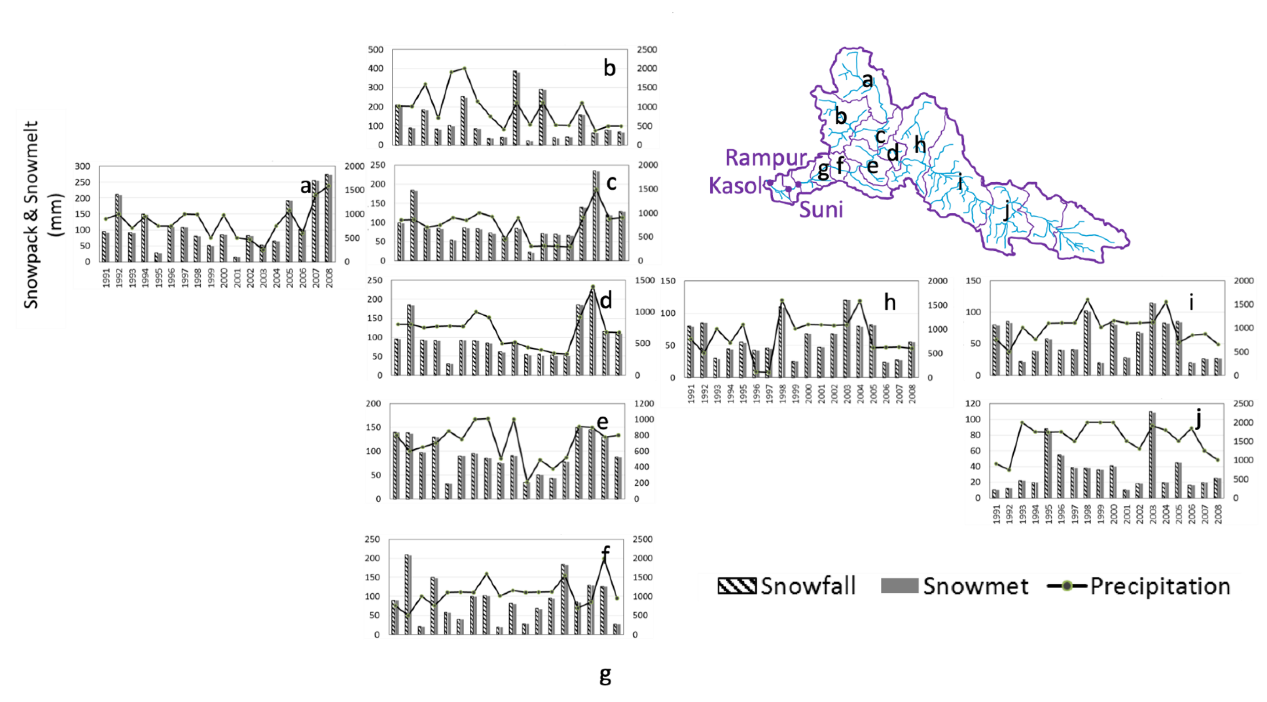
Considering that most of the drainage areas of this catchment are snowmelt-dependent and are upstream of Rampur station, a deeper assessment of snowfall and snowmelt along with streamflow generation is required at high altitudes given the lack of high-altitude station data. The temporal variability and spatial distribution of the hydrological components such as precipitation, snowpack, snowmelt, water yield (contributed by rainfall only), and total water yield (contributed by both snowmelt and rainfall) were computed and analyzed. Figure 4 illustrates the aggregation of simulated snowpack and snowmelt compared with precipitation from 1991 to 2008 in sub-catchments. Here, it is evident that the maximum snowpack contribution occurs at the sub-catchments, which correspond with high elevations. The sub-catchments such as SB1, SB2, SB3, SB4, SB15, and SB16 have varied their snowpack and snowmelt amount from ~10 to ~380 mm in a single year. Figure 3 shows that sub-catchments, such as SB10, SB11, SB12, and SB13, located in the lowest drainage areas, poorly contribute by snowpack, and consequently, the corresponding snowmelt is also poorly recorded. For these sub-catchments, the annual snowpack and corresponding melt amount were below 150 mm. Inter-annual changes in snowpack and the precipitation amount show local to large-scale influences in snow melt as well as snowpack. For example, SB1 shows that the proportion of snowmelt/snowpack with respect to precipitation was larger in 2000 and 2002, which contrasts with those proportions between 1995 and 1996. In the easternmost portion of the catchment, this proportion is consistent during all recorded years, which contrasts with the catchment’s lower drainage areas. Sorting the temperatures by the altitude, Figure 5 shows the possible influence of elevation differences along the catchment and through the year, which may respond to local-to-long-scale influences of climate patterns. Further analysis is required to identify causality in precipitation and temperature gradients in response to El Niño Southern Oscillation or inter-annual changes in monsoon intensity and inter-annual accumulation of snow.
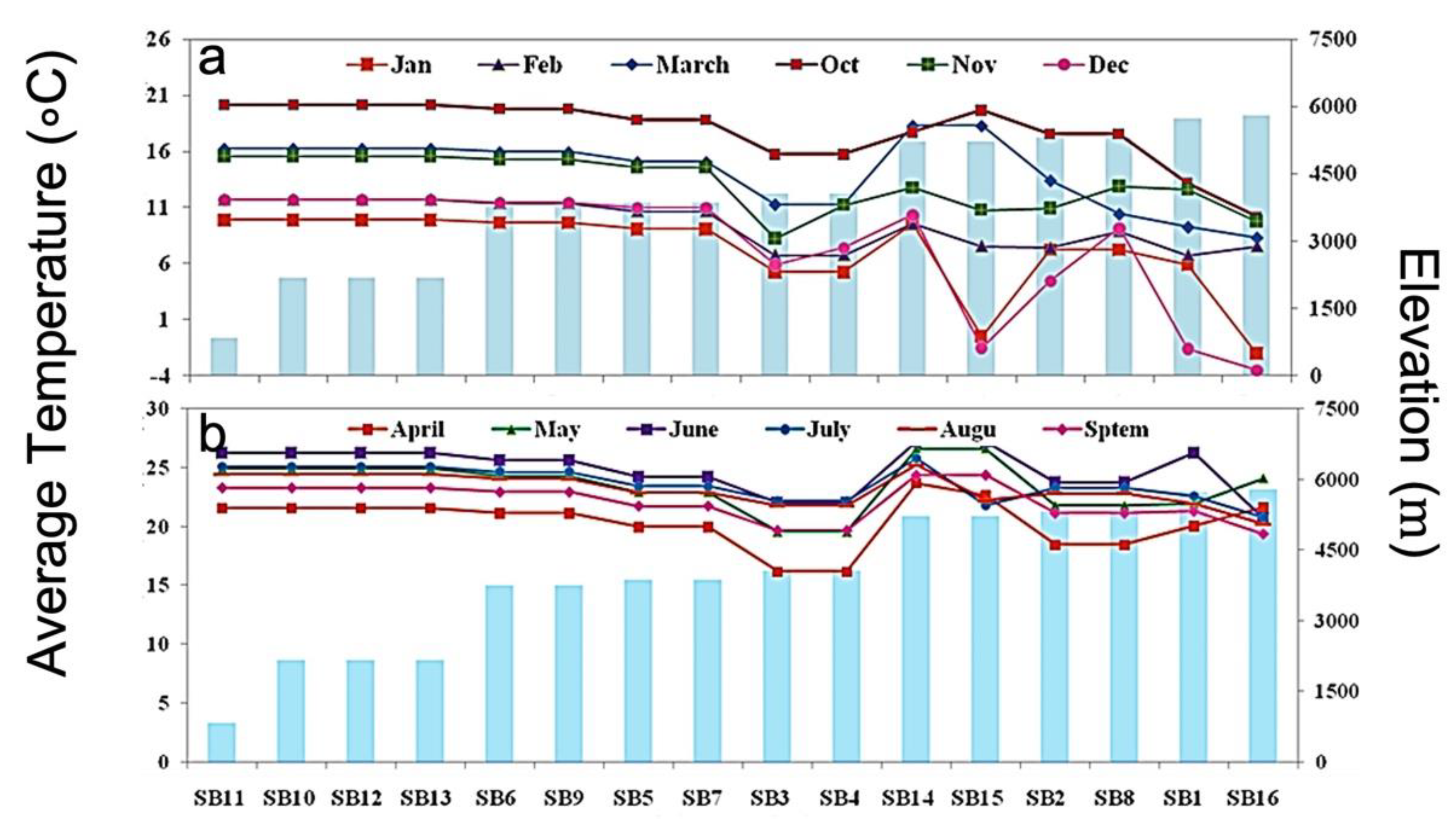
Spatiotemporal variations of temperature and precipitation along topographic gradients in the Himalayas, could drive the emergence or shift in hydrologic regimes [14]. During the near-term projection (2011–2030), the input parameters such as DEM, LULC, and soil map were kept constant to simulate and isolate possible effects of temperature and precipitation, which could emerge in places with highly variable elevations and large elevation gradients. The optimized parameter coefficient values are again incorporated in SWAT for the historical and near-term scenarios. The average annual TLR and PLR were estimated by elevation bands, as shown in Figure 5, and are incorporated in SWAT. The TLR and PLR are given as input to set up the SWAT model for sub-catchment calculations of snowfall and snowmelt, as well as parameters in calibration. Figure 5a,b illustrate the TLR or inverse changes in temperature with altitude [23]. Figure 5b also shows the winter and summer months temperature variations in relation to elevation differences, as well as the inherent variation due to seasonal cycles at each sub-catchment. While winter temperatures in low-altitude portions of the catchment vary between 9 °C and 21 °C, summer temperatures range between 22 °C and 27 °C. At high altitudes, the largest temperature span (21 °C) occurs during the winter months, whereas the summer months’ temperature span (5 °C) remains the same along the catchment. Parameter sensitivity in daily and monthly analyses (described in Table S2) evidenced SWAT’s ability to simulate flows in response to snowmelt rather than changes in temperatures. Figure 5b shows such sensitivity since the temperature between April and September remains within a 5 °C temperature span.
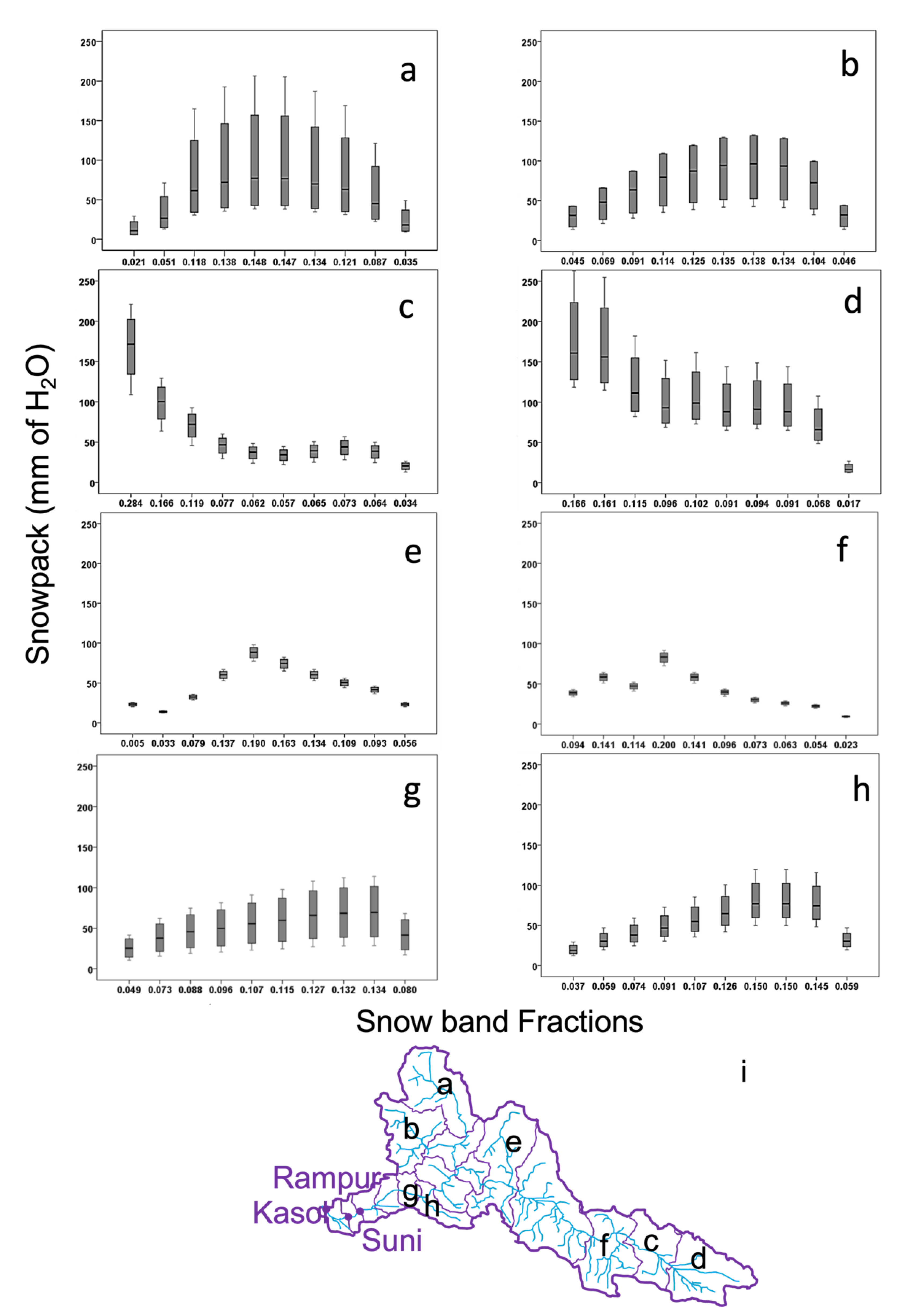
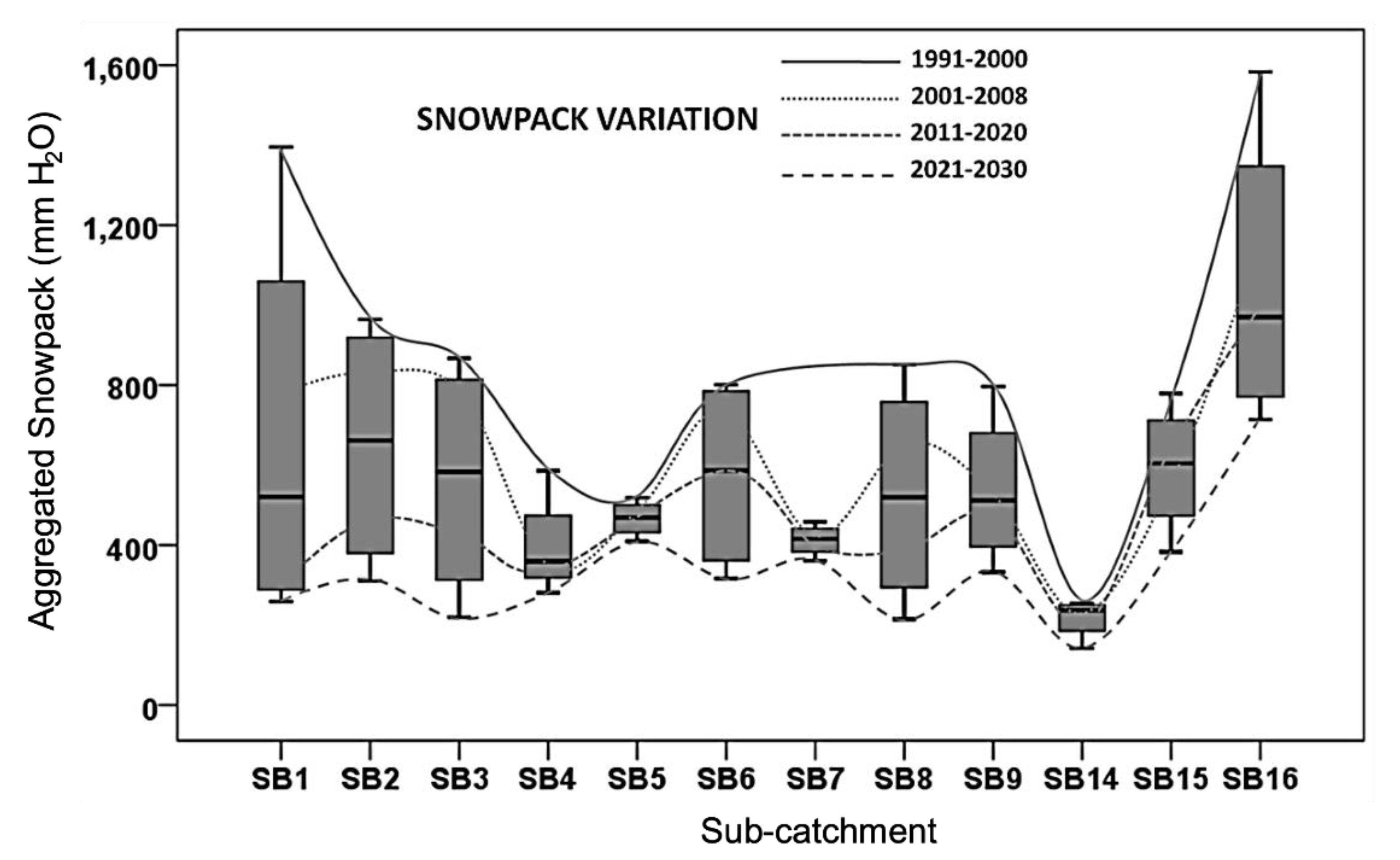
Changes in snowpack and variations in elevation bands are critical elements of modeling changes in snow accumulation. The variability of snow accumulation by snow band and altitude reflects the nonlinearity and high dimensionality of processes captured by the model parameterizations presented here. Figure 6 shows annual averages of snowpack variations by elevation band (10 Fractions) computed at each sub-catchment for the 1991–2030 period. These variations are expressed in the fractional snowpack at each sub-catchment, which at the same time define the variations in TLRs and PLRs. The distribution of the fractional snowpack varied throughout the catchment from upstream to downstream sub-catchments. Figure 6a–d are examples of high-altitude drainage areas characterized by high and variable snowpack. In contrast, low-land variations upstream of Rampur station (Figure 6e,f) evidenced small variability and low values of accumulated snow. Downstream of Rampur (Figure 6g,h) illustrate slightly larger variations in snow accumulation with average values below 50 mm/year. Figure 7 is consistent with the fractional variations in snowpack expressed above, expanding such variations into multi-decade contributions (1991–2000, 2001–2008, 2011–2020, and 2021–2030). In this figure, snowpack variation is highlighted at each catchment on a cumulative annual average. Figure 7 shows that sub-catchments at high elevations, such as SB1, SB2, SB3, SB8, SB15, and SB16, receive the highest amounts of snowpack. When compared intra-annually, the scenarios computed between 1991–2000 and 2001–2008 showed higher snowpack amounts than those calculated between 2011–2020 and 2021–2030. This difference in snowpack amount mainly occurred due to the variations in fractional snow covers.
Figure S1 shows the spatial distribution of multi-decadal averages of precipitation, snowpack, snowmelt, rainfall-runoff, and total water yields (contributed by both snowmelt runoff and rainfall runoff) for the period 1991–2008 and their differences with respect to the near-term period 2011–2030. Figure S2a shows that the lower portion of the catchment (i.e., SB10, SB11, SB12, and SB13) and the highest elevated part of the catchment (i.e., SB14, SB15, and SB16) had the largest precipitation (1991–2030); however, when compared with split time-series sets, such as the 1991–2008 and 2011–2030 time-series sets, precipitation decreases in the high elevation sub-catchments and increases in the lower elevation areas. The snowpack and snowmelt plots show similar trends in their time series. A decrease in the snowpack amounts can be observed in Figure S1b,c. Figure S2d also shows that the contribution of runoff (due to rainfall) has increased during the time 2011–2030. Figure S2e shows an increase in total water yield in sub-catchments at low elevations. The portions of the watershed most vulnerable to hydrologic changes, specifically, responses to variations in snow melting and snow accumulation, are the mid- to low-altitude portions of the catchment upstream of Rampur station.
Figure 8 illustrates the magnitude of change (shown as “% of change”) in snowpack amount as a function of the fraction of elevation bands. At each sub-catchment, the snowpack differences have been computed and analyzed by comparing historical and near-term scenarios. The results showed a significant decrease in snowpack amount across all the snowpack-induced sub-catchments. A 5% (minimum) to 42% (maximum) decrease in snowpack has been accounted for across all the sub-catchments. This shows the severity of temperature in snow cover and glaciers melting over Himalayan catchments. The sub-catchments SB1, SB2, SB3, SB8, and SB16 correspond with the utmost decrease in snowpack amount (20% to 42%); whereas the sub-catchments SB5, SB7, SB14, SB15, and SB16 showed a small to moderate decrease in snowpack amount (4% to 20%). It has been noticed that the SBs that are situated at a high elevation portion showed a higher amount of change or decrease in snowpack than the SBs, which are corresponded to moderate elevation ranges. This clearly illustrates a higher warming trend at high elevation portions than the moderate and low elevation ranges. The overall water balance components showed significant variations in the water yield, snowpack, and snowmelt over the Satluj river catchment.

4. Discussion

In this study, the role of elevations in snowpack and snowmelt computation are explored at sub-catchment-scale in the western Himalayas. Previous studies along the Himalayas have observed changes in snow accumulation and melting within the historical record [6,8,51,59]; however, it is unclear if snow parameterizations in hydrologic modeling can capture the nonlinearities of the snowpack formation and melt along complex topographic features. Ref. [60] explored the snowmelt runoff computational difficulties in a large complex terrain catchment. The strong variability in the degree-day factors from January to December has been reported by [20]. At the same time, such variation in the Satluj River Basin is evidenced by the maximum numbers of elevation bands (10 fractions) and maximum–minimum melt factors, which are incorporated at each sub-catchment scale, leading to improvements in the computation of snowmelt rate. The sub-catchment-wide distribution of elevation ranges increased the computation efficiency of the temperature index model, which complements earlier studies [9,20].
The fractional snowpack and snowmelt were computed at each elevation band and then their aggregation occurred at each sub-catchment outlet. The elevation bands contributed to identifying the reduction in the snowpack amount in response to elevation-dependent variations and (Figure 6 and Figure 8). SWAT-based inbuilt TLR and PLR parameters were formulated at each catchment scale by utilizing multiple elevation bands. The PLR and TLR were taken as calibration parameters, and after calibration, their optimized coefficient values significantly improved the model efficiency. Initially, Jain et al. (2008) used measured land surface temperature (LST) datasets to identify the role of TLR in the snowmelt process over the Satluj basin and reported that the TLR significantly affects the snowmelt over the Satluj basin. In this study, we also recognized the TLR as a significant sensitive parameter at each sub-catchment. The literature values suggested by [9] are used during calibration in the first iteration process.
Figure 2 shows a very good correlation at all gauges, even on the daily scale calibration in a very complex high hilly terrain Himalayan catchments (Table 2). As per [9,56], the R2 and NSE greater than 0.6 could be a reasonable agreement between the observed and simulated values, especially in the case of the Himalayan catchment (Table 2). Ref. [60] stated that the uncertainty estimation is an integral part of modeling studies, considering sources of uncertainty beyond the model to allow a realistic assessment of the degree of confidence that decision makers can have about potential outcomes. This study presented a rigorous approach to modeling calibration with uncertainty assessment. The present approach incorporated around 20 different hydrological calibration parameters relevant to surface water hydrology, groundwater hydrology, and snowmelt hydrology (Table S1).
The calibration was performed on both a monthly and daily basis, which significantly improved the accuracy of the simulated and projected snowmelt and snowpack (Table S2). The calibration of snow hydrological parameters significantly improved the modeling accuracy of snowmelt in the streamflow. The literature values related to snowmelt calibration parameters are helpful for the optimization process [9,15,20,50]. This study added multiple calibration parameters and performed a detailed sensitivity analysis to identify the most influencing model calibration parameters (Tables S1 and S2). The best-fit value of the most influencing parameter reduces the model uncertainty [32,56].
Ref. [61] worked on the Hindu-Kush-Karakoram Himalayan catchments and found that the satellite snow cover-based assessment of snowpack and snowmelt runoff is difficult in Himalayan catchments due to cloud covers and unavailability of field measurement datasets such as snow density and snow depths. Several authors found that the physical models, such as SWAT, which is based on real-time datasets, are fully able to compute the snowmelt and snowpack in the absence of satellite datasets over a large area catchment [28,49,51]; however, for small-scale study, incorporation of calibration parameters could be useful to improve the model accuracy [28,51,56]. The satellite-derived snow-cover-based computation of snow water equivalent (SWE) and snowmelt studies conducted by [15,20] were found comparable to the modeled snowmelt, as shown in Table 3. All studies reported that around a 60% snowmelt amount contributed to total runoff during summer, as observed in Figure 4. This justifies the overall accuracy of the present snowmelt modeling approach utilizing elevation bands; however, the fractional assessment of snowmelt and snowpack makes this study more reliable than previous studies [9,15,19,20,50], especially over the Himalayan catchment.
Many climate change studies revealed significant warming over Himalayan terrains and reported a significant reduction in snowpack and a higher melting rate of snow and glaciers [1,2,25]; therefore, in this study, GCM variables such as daily temperature and daily precipitation were used to project the near-term scenarios and our results revealed the same conclusion (Figure 8). The high elevation-based sub-catchments of the Satluj river basin show a significant reduction in snowpack amount and have been reported in previous studies [8,50,62]. In this study, we reported around 4% to 20% reduction in snowpack from the historical datasets and a maximum of up to 40% for the near-term scenarios at different elevation bands (or zones). The higher reduction in the snowpack has been observed at high elevation zones/catchments, similarly, reported by [62]. Ref. [53] also reported the earlier snow melting in case of higher warming and concluded that the snowpack would reduce around 4% to 18% with 2 °C increments in surface temperature. Similar observations were computed in the present study.

5. Conclusions

This study analyzed the snowpack and snowmelt computations in high elevations of the Satluj river Himalayan catchment. In this study, the snowpack and snowmelt were evaluated at multiple elevation bands, illustrating spatial variations in their amount at each sub-catchment. For the computation of snowpack and snowmelt, both measured and GCM datasets were used to highlight the intra-annual changes in snowmelt and snowpack. This study showed an enormous spatial and temporal variability in snowpack and snowmelt amount at each sub-catchment scale. The average TLR and PLR were successfully used to compute the more accurate estimation of snowpack and snowmelt. Various model calibration parameters were considered, and then sensitivity was analyzed. Based on the sensitivity analysis, significant sensitive and non-sensitive parameters were identified, which helped to improve the accuracy of the computation of snowpack and snowmelt. The other water balance components such as precipitation, water yield due to rainfall, and water yield due to snowmelt were spatial studies. The long-term spatial comparison of these water balance components showed noticeable spatial variability from upstream sub-catchments to downstream sub-catchments. The percentage of change analysis clearly showed that snowpack is highly variable over the Satluj catchment, and it could be more variable in the near-term period. Improvements in snowmelt runoff modeling capability using temperature index model and degree-day factors, the daily/diurnal variations in snowmelt rate will be incorporated by analyzing the effect of radiation factor, in which the rate and quantity of snowmelt depend on the surface as well as radiation factors. This work is underway. Furthermore, the relevance of this work worldwide may contribute to improving the diagnostics of winter floods and infrastructure resilience in places where snow storage and melting are critical to managing water resources [63,64].

Supplementary Materials

The following are available online at https://www.mdpi.com/article/10.3390/hydrology8040179/s1, Figure S1: (a) Soil and (b) Land use/Land cover maps of the Satluj river catchment, India; sub-catchment boundaries up to Kasol gauge. Figure S2: Changes and inter-annual comparisons in average annual (a) precipitation, (b) snowpack/snowfall, (c) snowmelt, (d) water yield (due to snow), and (e) total water yield (snowmelt and rainfall runoff) over the study area in different temporal climate domains (1991–2030), Table S1: Description of model calibration parameters, Table S2: Aggregate parameters values, their ranges, and global sensitivity results.

Author Contributions

Conceptualization, V.S. and F.M.-A.; methodology, V.S.; software, V.S.; validation, V.S.; formal analysis, V.S.; investigation, V.S. and F.M.-A.; resources, V.S. and F.M-A.; data curation, V.S.; writing—original draft preparation, V.S.; writing—review and editing, V.S. and F.M.-A.; visualization, V.S. and F.M.-A.; supervision, V.S. and F.M.-A.; project administration, V.S.; funding acquisition, V.S. and F.M.-A. All authors have read and agreed to the published version of the manuscript.

Funding

This research received no external funding.

Institutional Review Board Statement

Not applicable.

Informed Consent Statement

Not applicable.

Data Availability Statement

We just cited the multiple sources of data used and reported in the paper as results emerged from the proposed hypothesis testing.

Acknowledgments

We sincerely thank the India-WRIS project (RRSC-W, Indian Space Research Organization, India) and Central Water Commission (New Delhi, India) for providing the necessary data to successfully complete this research. We also thank the Intergovernmental Panel on Climate Change (IPCC) for providing the necessary GCM datasets for analysis. Some of the ideas were made possible through the Department of Science and Technology (DST), Govt. of India, the University of Nebraska-Lincoln (UNL), the Daugherty Water for Food Global Institute at the University of Nebraska (DWFI), and the Indo-U.S. Science and Technology Forum (IUSSTF). These institutions have partnered to nurture cooperation between students and scientists from India and the US through the Water Advanced Research and Innovation (WARI) Fellowship Program.

Conflicts of Interest

The authors declare no conflict of interest. The funders had no role in the design of the study; in the collection, analyses, or interpretation of data; in the writing of the manuscript, or in the decision to publish the results.

References

  1. Bolch, T.; Kulkarni, A.; Kääb, A.; Huggel, C.; Paul, F.; Cogley, J.G.; Frey, H.; Kargel, J.S.; Fujita, K.; Scheel, M.; et al. The state and fate of Himalayan glaciers. Science 2012, 336, 310–314. [Google Scholar] [CrossRef] [Green Version]
  2. Singh, V.; Jain, S.K.; Shukla, S. Glacier change and glacier runoff variation in the Himalayan Baspa River basin. J. Hydrol. 2021, 593, 125918. [Google Scholar] [CrossRef]
  3. Bhambri, R.; Bolch, T. Glacier mapping: A review with special reference to the Indian Himalayas. Prog. Phys. Geogr. 2009, 33, 672–704. [Google Scholar] [CrossRef] [Green Version]
  4. Xu, Y.; Ramanathan, V.; Washington, W.M. Observed high-altitude warming and snow cover retreat over Tibet and the Himalayas enhanced by black carbon aerosols. Atmos. Chem. Phys. 2016, 16, 1303–1315. [Google Scholar] [CrossRef] [Green Version]
  5. IPCC. Contribution of Working Group I to the Fifth Assessment Report of the Intergovernmental Panel on Climate Change. Climate Change 2013—The Physical Science Basis; Stocker, T.F., Qin, D., Plattner, G.K., Tignor, M., Allen, S.K., Boschungm, J., Nauels, A., Xia, Y., Bex, V., Midgley, P.M., Eds.; Cambridge University Press: Cambridge, UK; New York, NY, USA, 2013; p. 1535. [Google Scholar] [CrossRef] [Green Version]
  6. Singh, P.; Umesh, K.H.; Kumar, N. Modelling and estimation of different components of streamflow for Gangotri Glacier basin, Himalayas. Hydrol. Sci. J. 2008, 53, 309–322. [Google Scholar] [CrossRef]
  7. Siemens, K.; Dibike, Y.; Shrestha, R.R.; Prowse, T. Runoff Projection from an Alpine Watershed in Western Canada: Application of a Snowmelt Runoff Model. Water 2021, 13, 1199. [Google Scholar] [CrossRef]
  8. Shukla, S.; Jain, S.K.; Kansal, M.L. Hydrological modelling of a snow/glacier-fed western Himalayan basin to simulate the current and future streamflows under changing climate scenarios. Sci. Total Environ. 2021, 795, 148871. [Google Scholar] [CrossRef]
  9. Jain, S.K.; Tyagi, J.; Singh, V. Simulation of runoff and sediment yield for a Himalayan watershed using SWAT. J. Water Resour. Protect. 2010, 2, 267–281. [Google Scholar] [CrossRef]
  10. Zhang, Y.; Xu, C.Y.; Hao, Z.; Zhang, L.; Ju, Q.; Lai, X. Variation of Melt Water and Rainfall Runoff and Their Impacts on Streamflow Changes during Recent Decades in Two Tibetan Plateau Basins. Water 2020, 12, 3112. [Google Scholar] [CrossRef]
  11. Munoz-Arriola, F.; Lettenmaier, D.P.; Zhu, C.; Avissar, R. Water resources sensitivity of the Rio Yaqui Basin, México to agriculture extensification under multi-scale climate conditions. Water Resour. Res. 2009, 45, W00A20. [Google Scholar] [CrossRef]
  12. Muñoz Arriola, F.; Salgado Rabadán, J.H.; Rocchiccioli, H.M.; Shukla, S.; Güitrón De los Reyes, A.; Sánchez, L.R. Surface Hydrology in the Grijalva River Basin: Calibration of the Variable Infiltration Capacity Model. Aqua-LAC 2011, 3, 68–79. [Google Scholar] [CrossRef]
  13. Frans, C.; Istanbulluoglu, E.; Vimal, M.; Munoz-Arriola, F.; Lettenmaier, D.P. On runoff trends in the Upper Mississippi River Basin: Influences of climate and land use. Geophys. Res. Lett. 2013, 40, 1104–1110. [Google Scholar] [CrossRef]
  14. Khan, M.; Munoz-Arriola, F.; Shaik, R.; Greer, P. Spatial heterogeneity of temporal shifts in extreme precipitation across India. J. Clim. Chang. 2019, 5, 19–31. [Google Scholar] [CrossRef]
  15. Singh, P.; Jain, S.K. Snow and glacier melt in the Satluj River at Bhakra Dam in the western Himalayan region. Hydrol. Sci. J. 2002, 47, 93–106. [Google Scholar] [CrossRef]
  16. Mote, P.W.; Hamlet, A.F.; Lettenmaier, D.P. Variability and trends in mountain snowpack in western North America. In Proceedings of the Western Snow Conference, Richmond, BC, Canada, 19–22 April 2004; pp. 15–22. [Google Scholar]
  17. Mote, P.W. Climate-driven variability and trends in mountain snowpack in western North America. J. Clim. 2006, 19, 6209–6220. [Google Scholar] [CrossRef]
  18. Frans, C.; Istanbulluoglu, E.; Lettenmaier, D.P.; Naz, B.; Clarke, G.; Condom, T.; Burns, P.; Nolin, A. Predicting glacio-hydrologic change in the headwaters of the Zongo River, Cordillera Real, Bolivia. Water Resour. Res. 2015, 51, 9029–9052. [Google Scholar] [CrossRef]
  19. Jain, S.K.; Goswami, A.; Saraf, A.K. Accuracy assessment of MODIS, NOAA and IRS data in snow cover mapping under Himalayan conditions. Int. J. Remote Sens. 2008, 29, 5863–5878. [Google Scholar] [CrossRef]
  20. Tiwari, S.; Kar, S.C.; Bhatla, R. Examination of snowmelt over Western Himalayas using remote sensing data. Theor. Appl. Climatol. 2016, 125, 227–239. [Google Scholar] [CrossRef]
  21. Singh, V.; Goyal, M.K. Analysis and trends of precipitation lapse rate and extreme indices over north Sikkim eastern Himalayas under CMIP5ESM-2M RCPs experiments. Atmos. Res. 2016, 167, 34–60. [Google Scholar] [CrossRef]
  22. Singh, V.; Goyal, M.K. Changes in climate extremes by the use of CMIP5 coupled climate models over eastern Himalayas. Environ. Earth Sci. 2016, 75, 1–27. [Google Scholar] [CrossRef]
  23. Gardner, A.S.; Sharp, M.J.; Koerner, R.M.; Labine, C.; Boon, S.; Marshall, S.J.; Lewis, D. Near-surface temperature lapse rates over Arctic glaciers and their implications for temperature downscaling. J. Clim. 2009, 22, 4281–4298. [Google Scholar] [CrossRef]
  24. Gascoin, S. Snowmelt and Snow Sublimation in the Indus Basin. Water 2021, 13, 2621. [Google Scholar] [CrossRef]
  25. Change, I.C.; Working Group I Contribution to the Fifth Assessment. Climate Change 2013: The Physical Science Basis. Report of the Intergovernmental Panel on Climate Change; IPCC: Cambridge, UK; New York, NY, USA, 2013. [Google Scholar]
  26. Shrestha, B.; Babel, M.S.; Maskey, S.; van Griensven, A.; Uhlenbrook, S.; Green, A.; Akkharath, I. Impact of climate change on sediment yield in the Mekong River Catchment: A case study of the Nam Ou Catchment, Lao PDR. Hydrol. Earth Syst. Sci. 2013, 17, 1–20. [Google Scholar] [CrossRef] [Green Version]
  27. Fontaine, T.A.; Cruickshank, T.S.; Arnold, J.G. Development of a snowfall-snowmelt routine for mountainous terrain for the soil water assessment tool (SWAT). J. Hydrol. 2002, 262, 209–223. [Google Scholar] [CrossRef]
  28. Goyal, M.K.; Sarma, A.K. Analysis of the change in temperature trends in Subansiri River basin for RCP scenarios using CMIP5 datasets. Theor. Appl Climatol. 2017, 129, 1175–1187. [Google Scholar]
  29. Narsimlu, B.; Gosain, A.K.; Chahar, B.R. Assessment of future climate change impacts on water resources of Upper Sind River Catchment, India, using SWAT Model. Water Resour. Manag. 2013, 27, 3647–3662. [Google Scholar] [CrossRef]
  30. Beniston, M. Is snow in the Alps receding or disappearing? Wiley Interdiscip. Rev. Clim. Chang. 2012, 3, 349–358. [Google Scholar] [CrossRef] [Green Version]
  31. Sridhar, V.; Nayak, A. Implications of climate-driven variability and trends for the hydrologic assessment of the Reynolds Creek Experimental Watershed Idaho. J. Hydrol. 2010, 385, 183–202. [Google Scholar] [CrossRef] [Green Version]
  32. Singh, V.; Bankar, N.; Salunkhe, S.S.; Bera, A.K.; Sharma, J.R. Hydrological streamflow modeling on Tungabhadra catchment: Parameterization and uncertainty analysis using SWAT CUP. Curr. Sci. 2013, 104, 1187–1199. [Google Scholar]
  33. Ficklin, D.L.; Barnhart, B.L. SWAT hydrologic model parameter uncertainty and its implications for hydroclimatic projections in snowmelt-dependent watersheds. J. Hydrol. 2014, 27, R713–R715. [Google Scholar] [CrossRef] [Green Version]
  34. Amaranto, A.; Pianosi, F.; Solomatine, D.; Corzo-Perez, G.; Munoz-Arriola, F. Sensitivity Analysis of Hydroclimatic Controls of Data-driven Groundwater Forecast in Irrigated Croplands. J. Hydrol. 2020, 587, 124957. [Google Scholar] [CrossRef]
  35. Singh, S.; Kumar, R.; Bhardwaj, A.; Sam, L.; Shekhar, M.; Singh, A.; Kumar, R.; Gupta, A. Changing climate and glacio-hydrology in Indian Himalayan Region: A review. Wiley Interdiscip. Rev. Clim. Chang. 2016, 7, 393–410. [Google Scholar] [CrossRef] [Green Version]
  36. Neupane, R.P.; Yao, J.; White, J.D. Estimating the effects of climate change on the intensification of monsoonal-driven stream discharge in a Himalayan watershed. Hydrol Process. 2013, 28, 6236–6250. [Google Scholar] [CrossRef]
  37. Neitsch, S.L.; Arnold, J.G.; Kiniri, J.R.; Williams, J.R. Soil Water Assessment Tool Theoretical Documentation Version 9; Technical Report No. 406 for Texas Water Resources Institute; Texas A & M University: College Station, TX, USA, 2011. [Google Scholar]
  38. GLCF. Shuttle Radar Topography Mission (SRTM) Technical Guide; University of Maryland: College Park, MD, USA, 2005; Available online: https://cgiarcsi.community/data/srtm-90m-digital-elevation-database-v4-1/ (accessed on 2 December 2021).
  39. FAO. The Digitized Soil Map of the World and Derived Soil Properties (Version 3.6); FAO Land and Water Digital Media Series 1; FAO: Rome, Italy, 2007. [Google Scholar]
  40. Taylor, K.E.; Stouffer, R.J.; Meehl, G.A. An overview of CMIP5 and the experiment design. Bull. Am. Meteorol. Soc. 2012, 93, 485–498. [Google Scholar] [CrossRef] [Green Version]
  41. Qiao, L.; Pan, Z.; Herrmann, R.; Hong, Y. Hydrological variability and uncertainty of lower Missouri River Catchment under changing climate. J. Am. Water Resour. Assoc. (JAWRA) 2013, 50, 246–260. [Google Scholar] [CrossRef]
  42. Chen, D.; Zhang, P.; Seftigen, K.; Ou, T.; Giese, M.; Barthel, R. Hydroclimate changes over Sweden in the twentieth and twenty-first centuries: A millennium perspective. Geogr. Ann. Ser. A Phys. Geogr. 2021, 103, 103–131. [Google Scholar] [CrossRef]
  43. Apurv, T.; Mehrotra, R.; Sharma, A.; Goyal, M.K.; Dutta, S. Impact of climate change on floods in the Brahmaputra basin using CMIP5 decadal predictions. J. Hydrol. 2015, 527, 281–291. [Google Scholar] [CrossRef]
  44. Lu, G.Y.; Wong, D.W. An adaptive inverse-distance weighting spatial interpolation technique. Comput. Geosci. 2008, 34, 1044–1055. [Google Scholar] [CrossRef]
  45. Snell, S.E.; Gopal, S.; Kaufmann, R.K. Spatial interpolation of surface air temperatures using artificial neural networks: Evaluating their use for downscaling GCMs. J. Clim. 2000, 13, 886–895. [Google Scholar] [CrossRef]
  46. Thornton, P.K.; Van de Steeg, J.; Notenbaert, A.; Herrero, M. The impacts of climate change on livestock and livestock systems in developing countries: A review of what we know and what we need to know. Agric. Syst. 2009, 101, 113–127. [Google Scholar] [CrossRef]
  47. Mahmood, R.; Babel, M.S. Evaluation of SDSM developed by annual and monthly sub-models for downscaling temperature and precipitation in the Jhelum Catchment, Pakistan and India. Theor. Appl. Climatol. 2012, 113, 27–44. [Google Scholar] [CrossRef]
  48. Arnold, J.G.; Srinivasan, R.; Muttiah, R.S.; Williams, J.R. Large area hydrologic modeling and assessment—Part I: Model development. J. Am. Water Resour. Assoc. 1998, 34, 73–89. [Google Scholar] [CrossRef]
  49. Anderson, E.A. A Point Energy and Mass Balance Model of a Snow Cover; NOAA Technical Report NWS 19; NOAA: Silver Spring, MD, USA, 1976; p. 150. [Google Scholar]
  50. Jain, S.K.; Goswami, A.; Saraf, A.K. Determination of land surface temperature and its lapse rate in the Satluj River basin using NOAA data. Int. J. Remote Sens. 2008, 29, 3091–3103. [Google Scholar] [CrossRef]
  51. Grusson, Y.; Sun, X.; Gascoin, S.; Sauvage, S.; Raghavan, S.; Anctil, F.; Sáchez-Pérez, J.M. Assessing the capability of the SWAT model to simulate snow, snow melt and streamflow dynamics over an alpine watershed. J. Hydrol. 2015, 531, 574–588. [Google Scholar] [CrossRef]
  52. Abbaspour, K.C.; Yang, J.; Maximov, I.; Siber, R.; Bogner, K.; Mieleitner, J.; Zobrist, J.; Srinivasan, R. Modelling hydrology and water quality in the pre-alpine/alpine Thur watershed using SWAT. J. Hydrol. 2007, 333, 413–430. [Google Scholar] [CrossRef]
  53. Singh, P.; Kumar, N. Impact assessment of climate change on the hydrological response of a snow and glacier melt runoff dominated Himalayan River. J. Hydrol. 1997, 193, 316–350. [Google Scholar] [CrossRef]
  54. Yang, J.; Reichert, P.; Abbaspour, K.C.; Yang, H. Hydrological modelling of the Chaohe Catchment in China: Statistical model formulation and Bayesian inference. J. Hydrol. 2007, 340, 167–182. [Google Scholar] [CrossRef]
  55. Zhou, J.; Liu, Y.; Guo, H.; He, D. Combining the SWAT model with sequential uncertainty fitting algorithm for streamflow prediction and uncertainty analysis for the Lake Dianchi Catchment, China. Hydrol. Process. 2014, 28, 521–533. [Google Scholar] [CrossRef]
  56. Abbaspour, K.C. SWAT-CUP4: SWAT Calibration and Uncertainty Programs—A User Manual; Swiss Federal Institute of Aquatic Science and Technology (Eawag): Dübendorf, Switzerland, 2011. [Google Scholar]
  57. Tang, Q.; Vivoni, E.; Munoz-Arriola, F.; Lettenmaier, D.P. Predictability of evapotranspiration patterns using remotely-sensed vegetation dynamics during the North American monsoon. J. Hydrometeorol. 2012, 13, 103–121. [Google Scholar] [CrossRef]
  58. Amaranto, A.; Munoz-Arriola, F.; Corzo-Perez, G.; Solomatine, D. A Spatially enhanced data-driven multi-model to improve semi-seasonal groundwater forecasts in the High Plains aquifer, USA. Water Resour. Res. 2019, 55, 5941–5961. [Google Scholar] [CrossRef] [Green Version]
  59. Legates, D.R.; McCabe, G.J., Jr. Evaluating the use of “goodness-of-fit” measures in hydrologic and hydroclimatic model validation. Water Resour. Res. 1999, 35, 233–241. [Google Scholar] [CrossRef]
  60. Johnston, R.; Smakhtin, V. Hydrological modeling of large river basins: How much is enough? Water Resour. Manag. 2014, 28, 2695–2730. [Google Scholar] [CrossRef] [Green Version]
  61. Pellicciotti, F.; Buergi, C.; Immerzeel, W.W.; Konz, M.; Shrestha, A.B. Challenges and uncertainties in hydrological modeling of remote Hindu Kush–Karakoram–Himalayan (HKH) basins: Suggestions for calibration strategies. Mt. Res. Dev. 2012, 32, 39–50. [Google Scholar] [CrossRef]
  62. Shukla, S.; Kansal, M.L.; Jain, S.K. Snow cover area variability assessment in the upper part of the Satluj river basin in India. Geocarto Int. 2017, 32, 1285–1306. [Google Scholar] [CrossRef]
  63. Sarzaeim, P.; Ou, W.; de Oliveira, L.A.; Munoz-Arriola, F. Flood-Risk Analytics for Climate-Resilient Agriculture Using Remote Sensing in the Northern High Plains. Geo-Extreme 2021, 2021, 234–244. [Google Scholar] [CrossRef]
  64. Wilson, A.; Cifelli, R.; Munoz-Arriola, F.; Giovannettone, J.; Vano, J.; Parzybok, T.; Dufour, A.; Jasperse, J.; Mahoney, K.; McCormick, B. Efforts to Build Infrastructure Resiliency to Future Hydroclimate Extremes. Geo-Extreme 2020, 2020, 222–233. [Google Scholar] [CrossRef]
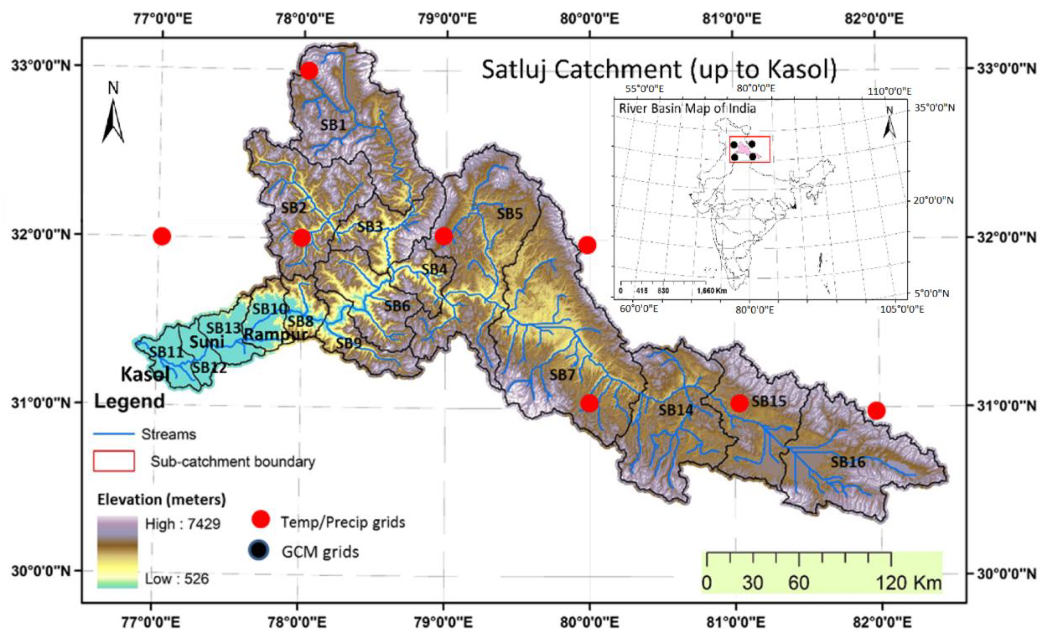
Figure 1. Topographic map and location of the Satluj river catchment, India; sub-catchment boundaries up to Kasol gauge.
Hydrology 08 00179 g001
Figure 2. Daily calibration (1991–2000) and validation (2001–2008) vs. observations at three outlets: (a) Rampur calibration; (b) Rampur validation; (c) Suni calibration; (d) Suni validation; (e) Kasol calibration; (f) Kasol validation.
Hydrology 08 00179 g002
Figure 3. Annual variability of snowpack and snowmelt and precipitation at sub-catchment scale for the year 1991 to 2008. Following drainage areas in Figure 1b, the stations above drain from left to right: (a) SB1: from top to bottom; (b) SB2; (c) SB3; (d) SB4; (e) SB6; (f) SB8: from (j) SB14 to (i) SB7: from right to left (i) SB7 to (h) SB5; and (g) SB13.
Hydrology 08 00179 g003
Figure 4. Averaged modeled daily discharge (1991–2008) at Kasol showing snowmelt-induced discharge and rainfall-induced discharge.
Hydrology 08 00179 g004
Figure 5. Changes of average temperatures along multiple sub-watersheds. The bar indicates the elevation of the centroid for (a) winter months and (b) summer months.
Hydrology 08 00179 g005
Figure 6. Sub-catchment snowpack changes computed as per elevation bands during whole time series (1991–2030): (a) SB1; (b) SB2; (c) SB15; (d) SB16; (e) SB5; (f) SB7; (g) SB8; (h) SB9; (i) sub-catchment location of the stations above. Selected sub-catchment respond to for distinct patterns across the Satluj River Basin.
Hydrology 08 00179 g006
Figure 7. Changes in aggregated snowpack by decade (lines) at each sub-basin. The lines just evidence the difference of aggregated snowpack between decades (there is no physical process that connects sub-basins in the order observed in the x-axis).
Hydrology 08 00179 g007
Figure 8. Percentage of change in snowpack amount (average annual) over different sub-catchments of Satluj river.
Hydrology 08 00179 g008
Table 1. SWAT model simulated water balance components details.
Model Simulation Details
General details Satluj catchment
Simulation period (years)16
Warm up (years)2
Hydrological response units (HRUs)358
Sub-basins16
Output time stepDaily, Monthly
Watershed area (km2)51,055
Water Balance Ratios
Streamflow/precipitation0.63
Baseflow/total flow0.25
Surface runoff/total flow0.45
Percolation/precipitation0.26
Deep recharge/precipitation0.01
ET/precipitation0.36
Water Balance Components (mm)
ET382.0
Precipitation1073.5
Surface runoff304.8
Lateral flow113.0
Return Flow259.0
Percolation to shallow aquifer283.4
Revaporation from shallow aquifer10.2
Recharge to deep aquifer14.2
Table 2. Model calibration and validation results as per SUFI method on the daily and monthly basis analysis.
Calibration (19912000)
Outlet StationDailyMonthly
p-Factorr-FactorR2NSEp-Factorr-FactorR2NSE
Rampur0.461.890.750.610.411.900.710.64
Kasol0.571.500.760.630.571.570.780.67
Suni0.521.600.720.590.491.430.730.60
Validation (2001–2008)
Outlet StationDailyMonthly
p-Factorr-FactorR2NSEp-Factorr-FactorR2NSE
Rampur0.431.890.620.540.451.920.650.55
Kasol0.521.670.710.590.601.620.730.61
Suni0.521.720.650.580.581.520.710.60
Table 3. Validation of modeled snowpack and snowmelt with respect to referenced datasets.
Variables SWATJain et al.,
2010
Singh and Kumar, 1997Tiwari et al., 2016Singh and Jain,
2002
Snowpack61% (Winter)65% (Winter)53% (summer)–64% (Winter)75% (Winter)59% (summer)–72% (Winter)
Snowmelt at Satluj 58%
(maximum)
59% (maximum)64%
(maximum)
63% (maximum)59% (maximum)
Publisher’s Note: MDPI stays neutral with regard to jurisdictional claims in published maps and institutional affiliations.