Article

Streamflow Reconstructions Using Tree-Ring Based Paleo Proxies for the Upper Adige River Basin (Italy)

1
Department of Civil, Environmental and Mechanical Engineering, Università degli Studi di Trento (UNITN), 77-38123 Trento, Italy
2
Department of Civil, Construction and Environmental Engineering, The University of Alabama (UA), Tuscaloosa, AL 35487, USA
3
Institute for Alpine Environment, Eurac Research, 39100 Bolzano, Italy
*
Author to whom correspondence should be addressed.
Hydrology 2022, 9(1), 8; https://doi.org/10.3390/hydrology9010008
Submission received: 1 December 2021 / Revised: 25 December 2021 / Accepted: 27 December 2021 / Published: 30 December 2021

Abstract

:
The Adige River Basin (ARB) provides a vital water supply source for varying demands including agriculture (wine production), energy (hydropower) and municipal water supply. Given the importance of this river system, information about past (paleo) drought and pluvial (wet) periods would quantity risk to water managers and planners. Annual streamflow data were obtained for four gauges that were spatially located within the upper ARB. The Old World Drought Atlas (OWDA) provides an annual June–July–August (JJA) self-calibrating Palmer Drought Severity Index (scPDSI) derived from 106 tree-ring chronologies for 5414 grid points across Europe from 0 to 2012 AD. In lieu of tree-ring chronologies, the OWDA dataset was used as a proxy to reconstruct both individual gauge and ARB regional streamflow from 0 to 2012. Principal component analysis (PCA) was applied to the four ARB streamflow gauges to generate one representative vector of regional streamflow. This regional streamflow vector was highly correlated with the four individual gauges, as coefficient of determination (R2) values ranged from 85% to 96%. Prescreening methods included correlating annual streamflow and scPDSI cells (within a 450 km radius) in which significant (p ≤ 0.01 or 99% significance) scPDSI cells were identified. The significant scPDSI cells were then evaluated for temporal stability to ensure practical and reliable reconstructions. Statistically significant and temporally stable scPDSI cells were used as predictors (independent variables) to reconstruct streamflow (predictand or dependent variable) for both individual gauges and at the regional scale. This resulted in highly skillful reconstructions of upper ARB streamflow from 0 to 2012 AD. Multiple drought and pluvial periods were identified in the paleo record that exceed those observed in the recent, historic record. Moreover, this study concurred with streamflow reconstructions in nearby European watersheds.

1. Introduction

Understanding the hydrological cycle in alpine regions is receiving more and more attention from the scientific community, especially in the context of climatic change, glacial evolution, extreme flood and droughts events, agriculture, and energy production [1,2,3,4]. The Alps are identified as the water towers of Europe, being the main source of fresh water for downstream areas, especially in the summer period [1,5]. Quantifying the drivers and the effects of hydrological extremes on water availability for water management and optimal allocation is an ongoing challenge, especially in snow-dominated environments [3,6]. The upper Adige River Basin (ARB) (Figure 1) is in the northeast region of the Italian Alps. The ARB has a drainage area of around 12,100 km2 and river length of around 410 km which is the third largest catchment and the second longest river in Italy [3,4,7]. The ARB covers two Italian regions (Trentino Alto-Adige and Veneto) and the upper part (Bolzano Province) accounts for around 62% of the entire catchment area [8,9,10]. The mean annual precipitation is highly variable across the basin [4], ranging between around 500 mm (in the northwest region of the basin) up to 1600 mm (in the southern region of the basin). The ARB is an example of a typical Alpine catchment, presenting: (i) strong elevation gradients and steep slopes, which in turn influence the spatial distribution of precipitation [11] and (ii) discharges with a minimum in the winter due to the snow accumulation and a maxima in late spring and autumn, due to snow melting and convective storms, respectively [3,4]. The ARB is one of the most important Italian rivers for: (i) biological and ecological richness, hosting several protected areas such as the Stelvio National Park and a large variety of habitats and natural species [12], and (ii) hydroelectric production, providing water for around 34 large hydropower plants with an average nominal capacity larger than 3 MW [13,14].
There are very few published studies of streamflow reconstructions using paleo proxies and, those studies that are published are in nearby regions including recent work by [15] focusing on the Rhine River Basin and Po River Basin. Ref. [15] observed mixed results in obtaining good reconstruction skill in the Rhine River Basin and poor reconstruction skill in the Po River Basin. That study attributed the poor Po River Basin reconstruction skill to the influences of Alpine runoff [15]. Ref. [16] reconstructed streamflow in fourteen European watersheds (basins) from 1500 to 2000 (note, the ARB was not included in the fourteen basins studied). Ref. [16] identified three years (1540, 1669 and 1921) as extreme drought years for these watersheds.
While traditional reconstructions of streamflow rely on tree-ring proxies, [17,18] developed a novel approach at both the basin scale (i.e., Missouri River Basin, U.S.) and the continental scale (i.e., Continental U.S. or CONUS), in which tree-ring based reconstructions of summer Palmer Drought Severity Index (PDSI) were used as reconstruction proxies. The PDSI data were obtained from the Living Blended Drought Atlas (LBDA) [19], an updated version of the North American Drought Atlas [20]. The LBDA has a spatial resolution of 0.5 degrees by 0.5 degrees across the CONUS. Ref. [17] selected a search radius of 450 km from the streamflow gauge of interest and considered all LBDA PDSI cells within this radius when developing reconstruction models. In Europe, the Old World Drought Atlas (OWDA) provides an annual June–July–August (JJA) self-calibrating Palmer Drought Severity Index (scPDSI) derived from 106 tree-ring chronologies for 5414 grid points across Europe from 0 to 2012 AD [21]. Similar to [15,16], this study used the OWDA scPDSI as reconstruction proxies for streamflow. Per [17], OWDA scPDSI cells within a 450 km radius of the centroid of the upper ARB were evaluated (pre-screened) for use in reconstruction models.
Perhaps the biggest challenge [17] was identified when utilizing the LBDA as a reconstruction proxy was the high spatial correlation of the LBDA grids cells, which could lead to multi-collinearity challenges with reconstruction model development. Various statistical techniques exist to determine the relationship between two, spatial-temporal fields including regularized canonical correlation analysis (rCCA), as selected by [17], and principal component analysis (PCA), as selected by [15], which are both very appropriate. This study selected PCA to generate a single, time-series vector that represents the variability of streamflow for the multiple gauges identified in the upper ARB (i.e., dependent variable) and, thus, a regional reconstruction of upper ARB streamflow could be performed. Moreover, [17] noted that, “A single reconstruction model would be advantageous in its ability to consider all streamflow stations at once rather than fitting 55 individual models.” Thus, the use of PCA will address a desire of [17] to generate a regional reconstruction instead of individual gauge reconstruction(s). A rigorous set of statistics was used to evaluate the regression models developed to test for over-fitting and multi-collinearity per [17].
Thus, the objective of this study is to (a) develop skillful reconstructions of annual streamflow in the upper ARB; (b) evaluate and quantity (rank) droughts for various periods (length of record); (c) compare the results of the upper ARB to recent research efforts in central Europe.

2. Materials and Methods

The methodology for developing the streamflow reconstructions begins with the collection of streamflow and scPDSI datasets. Streamflow data (annual average flowrate—m3/s) was the dependent variable in the forward-backwards stepwise linear regression model. Reconstructed scPDSI data was then collected and was the independent variable in the regression model. Prescreening (correlation and stability) was performed prior to inputting the scPDSI data into the regression model. Regression models were then developed and model fit (skill) was evaluated with an emphasis on evaluating the models for multi-collinearity and over-fitting.

2.1. Streamflow

Streamflow data was collected in the framework of the Alpine Drought Observatory project (https://edp-portal.eurac.edu/cdb_doc/ado/, accessed on 1 November 2021) and consists of the average annual flowrate (m3/s) for four gauges within the upper ARB (Figure 1, Table 1). Streamflow data consists of gauged data from both impaired and unimpaired watersheds to increase the spatial coverage within the upper ARB. A total of 59 gauges were evaluated and the use of annual streamflow (in lieu of daily, monthly, or seasonal streamflow) reduces the impacts of any impairments which are generally associated with small hydropower facilities. The use of this streamflow data was justified based on intercorrelations between the four gauges for the 1980 to 2012 period of record (33 years) exceeding 99% significance for all combinations. Principal component analysis (PCA) was applied to the four gauges to generate a single vector to represent regional upper ARB streamflow.

2.2. OWDA scPDSI Data

The Old World Drought Atlas (OWDA) provides an annual June–July–August (JJA) self-calibrating Palmer Drought Severity Index (scPDSI) for 5414 grid points across Europe from 0 to 2012 AD [21]. Similar to [17], this research utilizes the OWDA scPDSI as a proxy for upper ARB streamflow reconstructions and will include 252 scPDSI cells within a 450 km search radius of the centroid of the upper ARB.

2.3. Predictor Prescreening Methods

Two prescreening methods were used to identify the most suitable scPDSI data for use as predictors for the reconstruction models. First, we inspected correlation coefficients between annual streamflow for the four gauges (and the PCA generated regional annual streamflow vector) and scPDSI cells to identify significant (p ≤ 0.01 or 99% significance) scPDSI cells. The next pre-screening method involved temporal stability analysis by performing an 11-year moving correlation window, similar to [22], between annual streamflow for the four gauges (and the PCA generated regional annual streamflow vector) and scPDSI cells and, scPDSI cells containing negative 11-year correlation values were considered unstable and removed from analysis. This stability analysis increased the likelihood that reliable and practical streamflow reconstructions were generated.

2.4. Reconstruction Methodology

Statistical fitness of the scPDSI to estimate annual regional streamflow in the upper ARB was tested using a forward and backward (standard) stepwise linear regression (SLR) model. The model adds and removes predictors until all variables not in the model have p-values that are greater than the specified alpha-to-enter value and when all variables in the model have p-values that are less than or equal to the specified alpha-to-remove value. Following the procedure of [23,24,25], the F-level for a predictor chronology had to have a maximum p-value of 0.05 for entry and 0.10 for retention in our stepwise regression model. Standard statistical measures were used to establish the statistical skill of each streamflow reconstruction. The R2 value quantified the amount of variance in each model. The R2-predicted was calculated using leave-one-out-cross-validation, in which a single year or observation is removed when fitting the model. The leave-one-out-cross-validation was considered a more rigorous evaluation when compared to the split sample approach. As a result, the prediction errors are independent of the predicted value at the removed observation [26]. The variation inflation factor (VIF) indicates the extent to which multicollinearity is present in a regression analysis. Generally, a VIF value close to 1.0 indicates low correlation between predictors and is ideal for a regression model [27]. The Durbin–Watson (D–W) statistic was used to analyze the autocorrelation structure of model residuals [28]. The sign test [23,24], a nonparametric procedure to count the number of agreements and disagreements between instrumental and reconstructed flow, was used for additional model validation.

3. Results

Excellent overall model skill (i.e., performance) was obtained for the reconstruction of the four gauges (Table 1). Each of the statistics used to evaluate model skill (performance), multi-collinearity, and over-fitting (e.g., R2 > ~0.50; R2-predicted > ~0.40; VIF < 10 and prefer = ~1.0; Durbin–Watson > ~1.5 and <~2.5; Sign Test) exceeded established thresholds (Figure 2). The four gauges were consistent in identifying 2001 as a pluvial (wet) year and 2005 as a drought year (Figure 2). Each of these events (the 2001 pluvial year and the 2005 drought year) were ranked while including reconstructed streamflow. The 2001 year ranked #3, #1, #1, and #1 while the 2005 year ranked #58, #30, #43 and #30 for the Adige/Etsch (Toll), Adige/Etsch (Sigmundskron), Adige/Etsch (Branzoll) and Rienz (Vintl)—respectively. Thus, 2001 was perhaps the wettest year in the past ~2000 years, while 2005 was one of the most extreme driest (drought) years. The reconstructed streamflow (m3/s) for annual and various filters (5-year, 10-year, 20-year and 30-year) are provided (Figure 3, Figure 4, Figure 5 and Figure 6).
Per [17], a regional streamflow reconstruction is preferred, as it will provide a representation of streamflow for the entire watershed in lieu of a “gauge by gauge” analysis. Thus, we will focus on the results from the regional reconstruction (Table 1 and Table 2; Figure 7, Figure 8 and Figure 9). PCA was performed on the four upper ARB streamflow gauges using annual flow (m3/s) from 1980 to 2012 to generate one vector to represent regional upper ARB streamflow. The first component of the eigenvalue analysis of the correlation matrix accounted for 91% of the variance. This was further verified when correlating the PCA-generated regional streamflow vector with each individual gauge as R2 values ranged from 85% to 96% (Table 1). Thus, the regional streamflow vector generated by PCA was very effective in capturing annual streamflow variability for the upper ARB. The 450 km search radius per Ho et al. (2016) identified 252 scPDSI cells to be considered in the regional streamflow reconstruction. The first step in the pre-screening process was to correlate each of scPDSI cell with the PCA generated regional streamflow vector and retain only those scPDSI cells that achieve a minimum 99% significance (p ≤ 0.01). This resulted in 40 of the 252 scPDSI cells being considered (Figure 7). The second step in the pre-screening process was to perform stability analysis in which an 11-year moving-window correlation of the 40 scPDSI cell with the PCA generated regional streamflow vector was performed which resulted in 13 of the 40 scPDSI cells being considered (Figure 7).
These 13 scPDSI cells were next considered in the SLR regression model and the results provided a statistically strong reconstruction (Table 1). Each of the statistics used to evaluate model skill, multi-collinearity, and over-fitting (e.g., R2 > ~0.50; R2-predicted > ~0.40; VIF < 10 and prefer = ~1.0; Durbin–Watson > ~1.5 and <~2.5; sign test) exceeded established thresholds. Three of the 13 scPDSI cells were retained in the SLR model as identified in the regression equation (Table 1) and Figure 7. As displayed in Figure 8, the SLR model generally captures the variability of the PCA generated regional streamflow vector with the only “misses” being ~1990 and ~1996 when the SLR model over-estimates annual streamflow (Figure 8).
The reconstructed (per the SLR regression model) regional annual streamflow was standardized (e.g., mean = 0 and standard-deviation = 1) and various filters (e.g., 5-year, 10-year, 20-year and 30-year end-year) were applied (Figure 9). Table 2 provides the ranking (1 to 5) for the various filters (e.g., annual, 5-year, 10-year, 20-year and 30-year end-year) for the lowest flows (i.e., drought periods). As displayed in Figure 9 and Table 2, the majority of ranked drought events occurred in the paleo (pre-instrumental) timeframe. An extreme drought period was observed near the end of the 12th century that resulted in 5-year, 10-year, 20-year and 30-year end-year droughts being ranked. Two prolonged (e.g., 30-year) droughts were observed in the 15th century. Similar to the 12th century, the early-mid 19th century displayed a period of extreme drought. Perhaps of equal interest was the lack of extreme drought during the first ~1000 years of the reconstructed record. The period for 0 to ~1000 AD appears to display pluvial periods of streamflow although a drought period was identified in the early 4th century and early 6th century (Figure 9c–e) that was just outside the one to five ranking.

4. Discussion

This study developed statistically skillful reconstructions of upper ARB annual streamflow for four streamflow gauges and a regional reconstruction, incorporating the novel approaches of [15,16,17,18]. Ref. [15] developed annual streamflow reconstructions for twenty-seven streamflow sites with varying locations within the nearby Po River Basin, using data from the Global Flood Awareness System (GloFAS) [29]. The overall average R2 value for the twenty-seven streamflow sites was 0.36. The reconstruction skill (R2 value) in this study for the individual streamflow gauges ranged from 0.58 to 0.74 with an average R2 value of 0.65, while the regional reconstruction resulted in an R2 value of 0.73. Several factors likely attributed to the increased skill in this study:
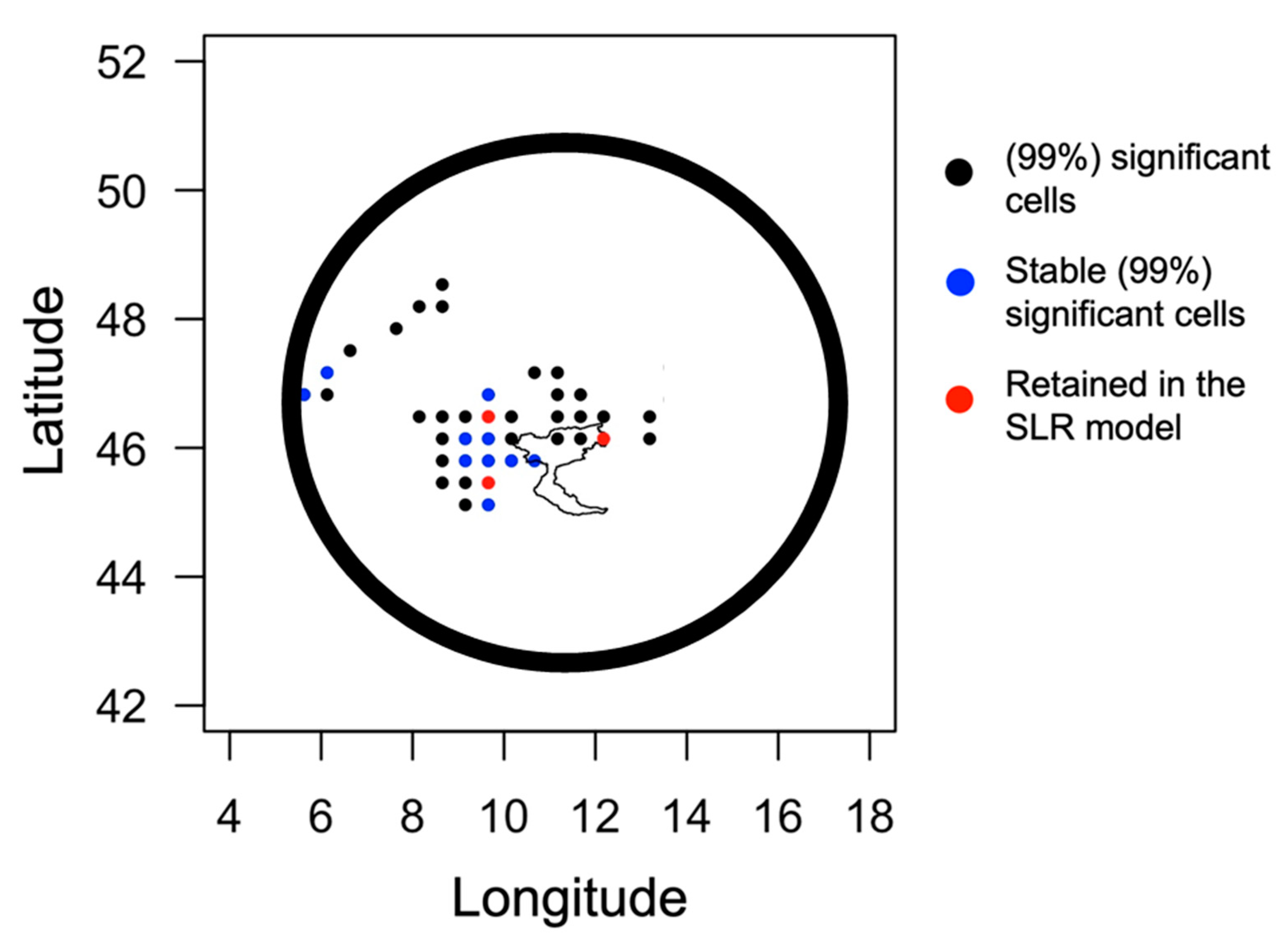
  • Adopted the recommendations of [17] in that a 450 km search radius was applicable to capture the regional climate signal when using scPDSI as proxies for streamflow reconstruction. Ref. [15] limited scPDSI cell to those (only) within the Po River Basin watershed. This limitation of scPDSI cells likely contributed to the lower Po River Basin reconstruction skill when compared to the upper ARB reconstruction skill obtained in this study. As displayed in Figure 6, the majority of scPDSI cells available for use in the SLR model are outside the ARB. Additionally, this pattern of scPDSI cells was consistently for the four individual ARB gauge locations (figures not provided). The regional climate signal appears to show scPDSI cells that are generally located west and north of the ARB. Physically, this confirms the generally pattern of moisture in this region (e.g., northern hemisphere) in which storms typically track from west to east. Thus, it is reasonable that the scPDSI cells identified as being “tele-connected” with ARB streamflow would be in the locations identified.
  • Obtained gauged streamflow data, while [15] utilized GloFAS-modeled streamflow data. The authors hypothesize the use of gauge data improved the skill of the streamflow reconstruction given that it represents an in-situ, measured data source and, thus, is likely to have fewer uncertainties when compared to GloFAS-modeled streamflow data. While the authors acknowledged that the gauge sites selected in the upper ARB likely have impairments, as stated, the use of this streamflow data was justified based on intercorrelations between the four gauges for the 1980 to 2012 period of record (33 years) exceeding 99% significance for all combinations. Thus, at an annual timescale, the gauges behave similarly and any impairments, primarily associated with small hydropower sites, appear minimal.
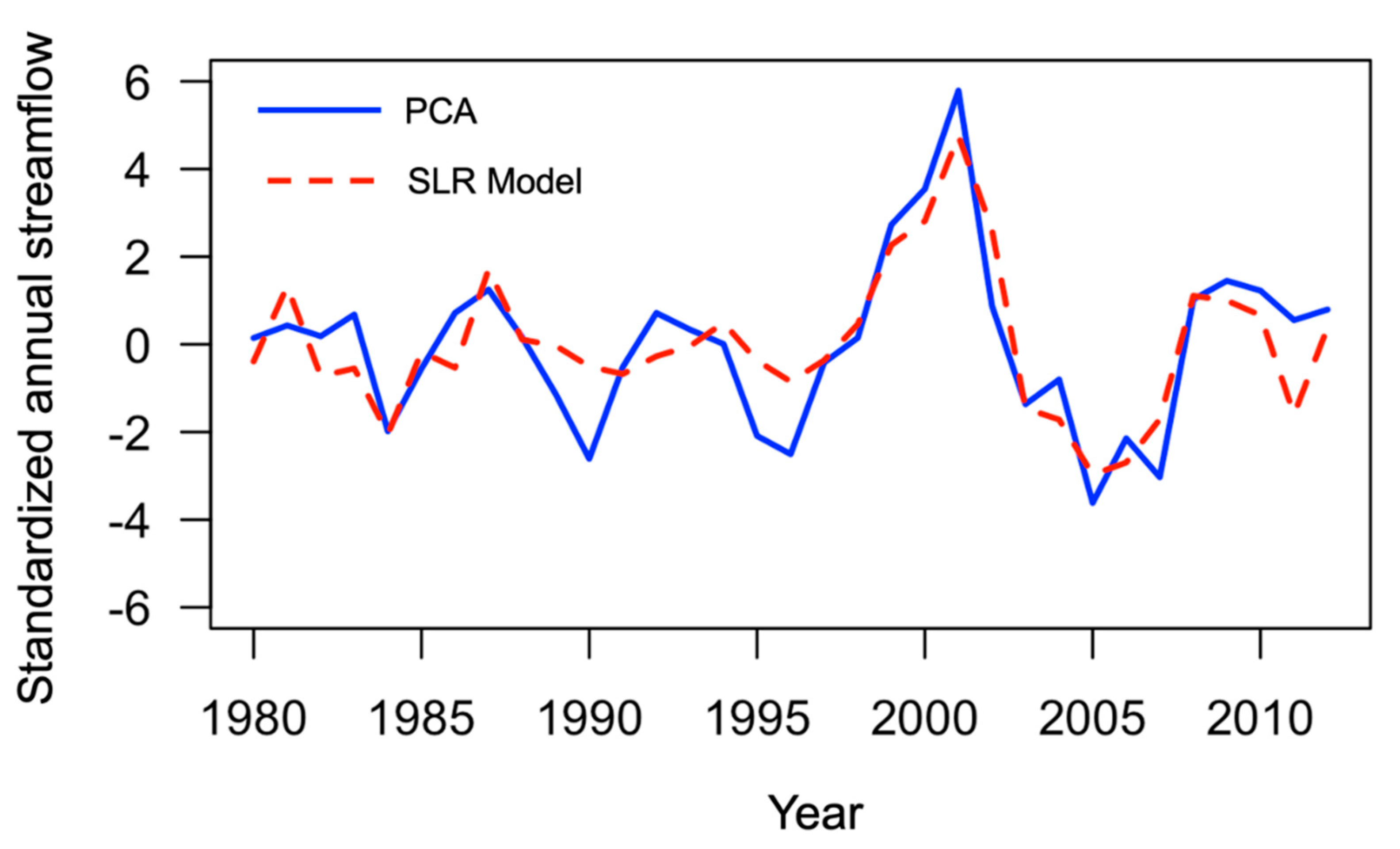
  • Developed a regional reconstruction in addition to the gauge reconstructions, which was recommended by [17]. We suspect that a regional representation of upper ARB streamflow will better capture a regional climate signal and, thus, provide increased statistical skill. The regional reconstruction resulted in an R2 value of 0.73 which was higher than three of the four individual gauges. The Adige/Etsch (Branzoll) streamflow reconstruction was the only gauge reconstruction to exceed the R2 value of the regional reconstruction and it exceeded it by only 0.01 (e.g., Adige/Etsch—Branzoll R2 value of 0.74).
  • We have high confidence in the regional reconstruction of annual upper ARB streamflow given rigorous statistical tests were performed to address concerns of multi-collinearity and over-fitting when using the highly intercorrelated scPDSI proxies.

5. Conclusions

The confidence in the current upper ARB reconstructions was further validated when compared to the recent European streamflow reconstructions using the OWDA scPDSI [16]. As previously stated, [16] identified drought years in the fourteen European watersheds (basins) in which streamflow reconstructions were generated from 1500 to 2000 (as noted, the upper ARB was not included in the fourteen basins). Ref. [16] identified three years (1540, 1669 and 1921) as extreme drought years. This study ranked individual drought years for 0 to 2012 AD, thus, increasing the period by ~1500 years when compared to [16] (Table 2). For the 2013-year period-of-record, the 1921 drought ranked #5, the 1540 drought #11 and the 1669 drought #100. Referring again to Table 2, when evaluating drought years from 1500 to 2012, which generally matches the period used by [16], the 1921 drought ranked #1, the 1540 drought #2 and the 1669 drought #21 (please note the “*” in the Table 2 rankings). Thus, this study confirmed in the upper ARB the extreme drought (specific years) that [16] identified in many watersheds across Europe. The upper ARB provides a vital water source for various and competing demands ranging from agriculture (e.g., grape and wine production) to energy (e.g., hydropower). This study provides important insight into the past variability of annual streamflow in the upper ARB, which, in turn, may be useful in future water allocations and planning.
Future research may explore extending the streamflow reconstructions into the middle ARB and lower ARB. Additionally, the paleo reconstructions should be compared to the recently released Intergovernmental Panel on Climate Change (IPCC) projections [30], such that a paleo perspective of future streamflow, based on various climate change scenarios, can be evaluated.

Author Contributions

Conceptualization, G.F. and G.T.; software, G.F.; validation, G.T.; formal analysis, G.T. and G.F.; investigation, G.T.; resources, G.T. and G.B.; data curation, G.F. and G.B.; writing—original draft preparation, G.T.; writing—review and editing, G.F., G.B. and G.T.; visualization, G.T. and G.F.; supervision, G.T.; project administration, G.T.; funding acquisition, G.T. All authors have read and agreed to the published version of the manuscript.

Funding

This research is supported by the National Science Foundation (NSF), Paleo Perspectives on Climate Change (P2C2) program award #18059590; the US—Italy J. William Fulbright Scholar program; Università di Trento; and The University of Alabama, Alabama Water Institute.

Institutional Review Board Statement

Not applicable.

Informed Consent Statement

Not applicable.

Data Availability Statement

Data for this study was accessed and available at the Alpine Drought Observatory project (https://edp-portal.eurac.edu/cdb_doc/ado/, accessed on 1 November 2021).

Acknowledgments

Tootle acknowledges the kind support and use of resources of the Alabama Water Institute of The University of Alabama and wishes to thank the members of the J. William Fulbright Scholarship Board; Julianne Cabour of the Institute of International Education; Barbara Pizzella and Chiara Petrilli of The U.S.—Italy Fulbright Commission; and Virna Eccli of the Università degli Studi di Trento for their support. The authors thank Doctor Eng. Daniela Quintero for providing the streamflow data which were collected by the Hydrographic Office of the Autonomous Province of Bolzano/Südtirol.

Conflicts of Interest

The authors declare no conflict of interest. The funders had no role in the design of the study; in the collection, analyses, or interpretation of data; in the writing of the manuscript, or in the decision to publish the results.

References

  1. Mastrotheodoros, T.; Pappas, C.; Molnar, P.; Burlando, P.; Manoli, G.; Parajka, J.; Fatichi, S. More green and less blue water in the Alps during warmer summers. Nat. Clim. Chang. 2020, 10, 155–161. [Google Scholar] [CrossRef]
  2. Puspitarini, H.D.; François, B.; Zaramella, M.; Brown, C.; Borga, M. The impact of glacier shrinkage on energy production from hydropower-solar complementarity in alpine river basins. Sci. Total Environ. 2020, 719, 137488. [Google Scholar] [CrossRef]
  3. Mallucci, S.; Majone, B.; Bellin, A. Detection and attribution of hydrological changes in a large Alpine river basin. J. Hydrol. 2019, 575, 1214–1229. [Google Scholar] [CrossRef]
  4. Galletti, A.; Avesani, D.; Bellin, A.; Majone, B. Detailed simulation of storage hydropower systems in large Alpine watersheds. J. Hydrol. 2021, 603, 127125. [Google Scholar] [CrossRef]
  5. Viviroli, D.; Dürr, H.H.; Messerli, B.; Meybeck, M.; Weingartner, R. Mountains of the world, water towers for humanity: Typology, mapping, and global significance. Water Resour. Res. 2007, 43. [Google Scholar] [CrossRef] [Green Version]
  6. Bocchiola, D. Long term (1921–2011) hydrological regime of Alpine catchments in Northern Italy. Adv. Water Resour. 2014, 70, 51–64. [Google Scholar] [CrossRef]
  7. Tuo, Y.; Marcolini, G.; Disse, M.; Chiogna, G. Calibration of snow parameters in SWAT: Comparison of three approaches in the Upper Adige River basin (Italy). Hydrol. Sci. J. 2018, 63, 657–678. [Google Scholar] [CrossRef]
  8. Gaglio, M.; Aschonitis, V.; Castaldelli, G.; Fano, E.A. Land use intensification rather than land cover change affects regulating services in the mountainous Adige river basin (Italy). Ecosyst. Serv. 2020, 45, 101158. [Google Scholar] [CrossRef]
  9. Tuo, Y.; Zheng, D.; Disse, M.; Chiogna, G. Evaluation of precipitation input for SWAT modeling in Alpine catchment: A case study in the Adige river basin (Italy). Sci. Total Environ. 2016, 573, 66–82. [Google Scholar] [CrossRef] [Green Version]
  10. Callegari, M.; Mazzoli, P.; De Gregorio, L.; Notarnicola, C.; Pasolli, L.; Petitta, M.; Pistocchi, A. Seasonal river discharge forecasting using support vector regression: A case study in the Italian Alps. Water 2015, 7, 2494–2515. [Google Scholar] [CrossRef] [Green Version]
  11. Formetta, G.; Marra, F.; Dallan, E.; Zaramella, M.; Borga, M. Differential orographic impact on sub-hourly, hourly, and daily extreme precipitation. Adv. Water Resour. 2021, 159, 104085. [Google Scholar] [CrossRef]
  12. Nagy, L.; Grabherr, G.; Körner, C.; Thompson, D.B. (Eds.) Alpine Biodiversity in Europe, 2003rd ed.; Springer Science Business Media: Berlin, Germany, 2012; Volume 167, Softcover reprint (512 pages) of the original 1st ed. [Google Scholar]
  13. Autorità di bacino del Fiume Adige, A.D.B. Quaderno Sul Bilancio Idrico Superficiale di Primo Livello; Bacino Idrografico Del Fiume Adige: Trento, Italy, 2008. [Google Scholar]
  14. Chiogna, G.; Majone, B.; Paoli, K.C.; Diamantini, E.; Stella, E.; Mallucci, S.; Bellin, A. A review of hydrological and chemical stressors in the Adige catchment and its ecological status. Sci. Total Environ. 2016, 540, 429–443. [Google Scholar] [CrossRef] [PubMed] [Green Version]
  15. Obertelli, M. A Data-Driven Approach to Streamflow Reconstruction Using Dendrochronological Data. Politecnico Milano Master Thesis by Marco Obertilli Matr. 2020, p. 899999. Available online: https://www.politesi.polimi.it/handle/10589/154385 (accessed on 1 November 2021).
  16. Nasreen, S.; Součková, M.; Vargas Godoy, M.R.; Singh, U.; Markonis, Y.; Kumar, R.; Hanel, M. A 500-year runoff reconstruction for European catchments. Earth Syst. Sci. Data Discuss. 2021, 1–29. [Google Scholar] [CrossRef]
  17. Ho, M.; Lall, U.; Cook, E.R. Can a paleodrought record be used to reconstruct streamflow?: A case study for the Missouri River Basin. Water Resour. Res. 2016, 52, 5195–5212. [Google Scholar] [CrossRef] [Green Version]
  18. Ho, M.; Lall, U.; Sun, X.; Cook, E.R. Multiscale temporal variability and regional patterns in 555 years of conterminous U.S. streamflow. Water Resour. Res. 2017, 53, 3047–3066. [Google Scholar] [CrossRef]
  19. Cook, E.R.; Seager, R.; Heim, R.R.; Vose, R.S.; Herweijer, C.; Woodhouse, C. Megadroughts in North America: Placing IPCC projections of hydroclimatic change in a long-term paleoclimate context. J. Quat. Sci. 2010, 25, 48–61. [Google Scholar] [CrossRef] [Green Version]
  20. Cook, E.R.; Krusic, P.J. The North American Drought Atlas, Lamont-Doherty Earth Observatory and National Science Foundation, N. Y. 2004. Available online: https://iridl.ldeo.columbia.edu/SOURCES/.LDEO/.TRL/.NADA2004/pdsiatlashtml/pdsireadme.html (accessed on 1 November 2021).
  21. Cook, E.R.; Seager, R.; Kushnir, Y.; Briffa, K.R.; Büntgen, U.; Frank, D.; Krusic, P.J.; Tegel, W.; Van Der Schrier, G.; Andreu-Hayles, L.; et al. Old World megadroughts and pluvials during the Common Era. Sci. Adv. 2015, 1, e1500561. [Google Scholar] [CrossRef] [PubMed] [Green Version]
  22. Biondi, F.; Waikul, K. DENDROCLIM2002: A C++ program for statistical calibration of climate signals in tree-ring chronologies. Comput. Geosci. 2004, 30, 303–311. [Google Scholar] [CrossRef]
  23. Vines, M.; Tootle, G.; Terry, L.; Elliott, E.; Corbin, J.; Harley, G.L.; Therrell, M. A Paleo Perspective of Alabama and Florida (USA) Interstate Streamflow. Water 2021, 13, 657. [Google Scholar] [CrossRef]
  24. Anderson, S.; Ogle, R.; Tootle, G.; Oubeidillah, A. Tree-ring reconstructions of streamflow for the Tennessee Valley. Hydrology 2019, 6, 34. [Google Scholar] [CrossRef] [Green Version]
  25. Woodhouse, C.A. A 431-Yr reconstruction of Western Colorado snowpack from tree rings. J. Clim. 2003, 16, 1551–1561. [Google Scholar] [CrossRef]
  26. Garen, D.C. Improved techniques in regression-based streamflow volume forecasting. J. Water Resour. Plan. Manag. 1992, 118, 654–670. [Google Scholar] [CrossRef]
  27. O’Brien, R.M. A caution regarding rules of thumb for variance inflation factors. Qual. Quant. 2007, 41, 673–690. [Google Scholar] [CrossRef]
  28. Draper, N.R.; Smith, H. Applied Regression Analysis, 2nd ed.; John Wiley: New York, NY, USA, 1981; p. 736. [Google Scholar]
  29. Harrigan, S.; Zsoter, E.; Alfieri, L.; Prudhomme, C.; Salamon, P.; Wetterhall, F.; Pappenberger, F. GloFAS-ERA5 operational global river discharge reanalysis 1979—Present. Earth Syst. Sci. Data 2020, 12, 2043–2060. [Google Scholar] [CrossRef]
  30. Intergovernmental Panel on Climate Change (IPCC) Climate Change 2021, They Physical Basis, Chapter 8 Water Cycle Changes. Available online: https://www.ipcc.ch/report/ar6/wg1/downloads/report/IPCC_AR6_WGI_Chapter_08.pdf (accessed on 1 November 2021).
Figure 1. Location map showing the four upper ARB streamflow stations and ARB watershed.
Hydrology 09 00008 g001
Figure 2. Observed (solid line) and SLR modeled (dashed line) annual flowrate (m3/s) from 1980 to 2012 for (a) Adige/Etsch (Toll), (b) Adige/Etsch (Sigmundskron), (c) Adige/Etsch (Branzoll), and (d) Rienz (Vintl). Coefficient of Determination (R2) is provided.
Hydrology 09 00008 g002
Figure 3. Reconstructed Adige/Etsch (Toll)—Year versus Flowrate (m3/s) from 0 to 2012 AD for (a) Annual, (b) 5-year, (c) 10-year, (d) 20-year and (e) 30-year end-year filters.
Hydrology 09 00008 g003
Figure 4. Reconstructed Adige/Etsch (Sigmundskron)—Year versus Flowrate (m3/s) from 0 to 2012 AD for (a) Annual, (b) 5-year, (c) 10-year, (d) 20-year and (e) 30-year end-year filters.
Hydrology 09 00008 g004
Figure 5. Reconstructed Adige/Etsch (Branzoll)—Year versus Flowrate (m3/s) from 0 to 2012 AD for (a) Annual, (b) 5-year, (c) 10-year, (d) 20-year and (e) 30-year end-year filters.
Hydrology 09 00008 g005
Figure 6. Reconstructed Rienz (Vintl)—Year versus Flowrate (m3/s) from 0 to 2012 AD for (a) Annual, (b) 5-year, (c) 10-year, (d) 20-year and (e) 30-year end-year filters.
Hydrology 09 00008 g006
Figure 7. The circular black line represents the 450 km search radius while the Adige River Basin watershed is provided. The three red circles represent scPDSI cells retained in the SLR model; the ten blue circles represent scPDSI stable cells that were not retained in the SLR model; and the twenty-seven black circles represent significant (99%) cells that were not stable.
Hydrology 09 00008 g007
Figure 8. Reconstructed annual standardized streamflow and PCA generated regional annual streamflow vector for overlapping (1980 to 2012) period.
Hydrology 09 00008 g008
Figure 9. Reconstructed regional streamflow standardized from 0 to 2012 AD for (a) Annual, (b) 5-year, (c) 10-year, (d) 20-year and (e) 30-year end-year filters.
Hydrology 09 00008 g009
Table 1. Streamflow stations, Latitude, Longitude, R2, R2—predicted, Variation Inflation Factor (VIF), Durbin-Watson, R2 (individual gauge versus PCA generated regional annual streamflow vector) and Regression Equation for Regression Model (scPDSI cell number in parenthesis).
StationLat, LonR2R2—PredictedVIFDurbin-WatsonSign TestR2Regression Equation
Adige/Etsch—Toll46.6764° N,
11.0835° E
0.580.491.1 (pass)1.95 (pass)18/15 (pass)85%Q = 32.958 + 1.644(70) + 1.060(98)
Adige/Etsch—Sigmundskron46.4856° N,
11.2988° E
0.640.581.1 (pass)1.42 (pass)17/16 (pass)93%Q = 53.8 + 2.26(81) + 2.19(154)
Adige/Etsch—Branzoll46.4040° N,
11.3206° E
0.740.691.1 (pass)1.70 (pass)17/16 (pass)96%Q = 139.55 + 4.7(81) + 6.9(154)
Rienz—Vintl46.8167° N,
11.7230° E
0.650.591.4 (pass)1.64 (pass)18/15 (pass)88%Q = 42.628 + 0.972(70) + 1.568(154)
Regional—PCAN/A0.730.661.1 (pass)1.69 (pass)14/19 (pass)N/AQ = −0.191 + 0.326(81) + 0.252(84) + 0.5288(154)
Table 2. Drought periods for the upper ARB regional reconstruction from 0 to 2012 AD. The number in the parenthesis represents the drought period ranking from 0 to 2012 AD while the number in the parenthesis with the “*” represents the drought period ranking from 1500 to 2012 AD.
Period1-Year5-Year10-Year20-Year30-Year
0 to 100
100 to 101
201 to 300
301 to 400375 (2)
401 to 500 485 (3)
501 to 600
601 to 700619 (4)
701 to 800
801 to 900
901 to 1000 988–969 (5)
1001 to 1100 1078–1069 (5)1079–1060 (2)1087–1058 (2)
1101 to 12001102 (1)1106–1102 (3)
1167–1163 (1)
1170–1161 (1)
1108–1099 (4)
1179–1160 (3)1185–1156 (5)
1201 to 1300
1301 to 1400 1397–1393 (2)1397–1388 (2)
1401 to 1500 1505–1501 (5) 1419–1390 (3)
1474–1445 (4)
1501 to 16001540 (11) (* 2)
1601 to 17001669 (100) (* 21)
1701 to 1800
1801 to 1900 1836–1832 (4)1844–1835 (3)1821–1802 (4)
1851–1832 (1)
1861–1832 (1)
1901 to 20121921 (5) (* 1)
Publisher’s Note: MDPI stays neutral with regard to jurisdictional claims in published maps and institutional affiliations.

