Article

Comparison of Regionalisation Techniques for Peak Streamflow Estimation in Small Catchments in the Pilbara, Australia

1
School of Geography Earth and Atmospheric Sciences, University of Melbourne, Parkville, VIC 3010, Australia
2
Alluvium Consulting, Level 1, 105-115 Dover Street, Cremorne, VIC 3121, Australia
*
Author to whom correspondence should be addressed.
Hydrology 2022, 9(10), 165; https://doi.org/10.3390/hydrology9100165
Submission received: 25 August 2022 / Revised: 13 September 2022 / Accepted: 22 September 2022 / Published: 24 September 2022

Abstract

:
Arid and semi-arid regions typically lack high-resolution river gauging data causing difficulties in understanding rainfall-runoff patterns. A common predictive method for discharge estimation within ungauged catchments is regional flood frequency estimation (RFFE), deriving peak discharge estimates from similar, gauged catchments and applying them to the catchment of interest. The majority of RFFE equations are developed for larger catchments where flow events may be larger and of greater interest. We test a series of RFFE methods derived for the Pilbara region, applying them to new ungauged small catchments under 10 km2. Rainfall values are derived from a guideline Australian design rainfall database, Australian Rainfall and Runoff 2019 (ARR2019) which was recently updated with an additional 30 years of rainfall data. RFFE equations are compared to a direct rainfall model to evaluate their performance within small catchments, identifying key limitations and considerations when modelling small headwater catchments.

1. Introduction

Flood frequency analysis is commonly undertaken to identify and estimate flood quantiles corresponding to a given return period using the available streamflow observations in a catchment [1]. Where streamflow records are absent, or catchments are widely ungauged, prediction of streamflow involves applying regional flood frequency estimation (RFFE) methods, which are data-driven empirical procedures that attempt to compensate for a lack of temporal data at a given location with spatial data, obtained from other locations within a homogenous region [2]. RFFE approaches are frequently used throughout Australia for the prediction of flood events. Accurately predicting the magnitude of flood events is essential for the planning of water resource systems [3] in addition to adhering to the design standards of engineered structures designed to convey a certain flow [4,5]. A lack of long-term rainfall and streamflow data within arid and semi-arid regions is a major issue for run-off modelling [6] and this challenge is highlighted here within the Pilbara region in Western Australia.
Western Australia accounts for 39% of the global supply of iron ore [7] but has a notable lack of rainfall and streamflow data owing to (a) the high spatial and temporal variability of streamflow, (b) the high cost of establishing dense hydrologic gauging sites (c) the likelihood of gauging sites being destroyed by flash flooding events and (d) the disproportionate interest of flow events in larger river channels resulting in a scarcity of data smaller catchments. This data scarcity results in a fewer opportunities for validation of hydrological models used and therefore there are limited opportunities to demonstrate that a given-site specific model is capable of making accurate predictions for periods outside a calibration period [8]. Nevertheless, increasing engineering modifications are carried out in small catchments in the Pilbara, such as culvert installation for roads and railways or mining river diversions—such as those found in our study region. River diversions are expensive engineering structures and their design and performance rely on adequately estimating both frequent and rare flow events [9]. There is also increased recognition of the importance to estimate and subsequently preserve natural hydrologic flow conditions resulting in an interest in estimating frequent flow events (e.g., 1EY, 0.5EY and 0.2EY where EY stands for the average number of exceedances per year) particularly in these semi-arid areas where flow is sparse and poorly understood.
Current practices for the design and prediction of peak discharges for river relocation designs are based on several estimation methods such as regionalisation methods, numerical and hydrologic modelling. The outcome of these methodological provides wide-ranging, typically heuristic results. However, the improvement of two-dimensional hydrodynamic models is changing how peak discharges are being estimated. Direct rainfall modelling (or rain-on-grid) has increasingly become a standard approach for predicting design flood behaviour [10,11]. The application of rainfall directly onto a 2D domain allows for the simulation of catchment runoff by applying it directly to the modelling grid [12,13]. Catchment runoff within direct rainfall models is dependent on the grid or mesh cell area, the rainfall depth, grid cell roughness, rainfall losses (IL/CL) and the slope between neighbouring cells. This distributed rainfall approach directly onto the 2D domain can give considerably more detail, particularly in the upper parts of sub-catchments [14] and has been found to provide a better representation of minor overland flowpaths than conventional modelling methods [12]. In the absence of stream gauges, this paper examines the suitability of direct rainfall modelling to test the suitability of RFFE approaches on small ungauged catchments within the Pilbara. The tested RFFE approaches were previously designed for the semi-arid Pilbara region and have previously been validated using gauged flow data within medium to large catchments [15,16,17,18]. Most direct-rainfall models are used as a means of indirect calibration or comparison with traditional hydrological predictive methods and can be used to elucidate discrepancies in other models [19]. Direct rainfall models are useful in the modelling of design flood simulations providing appropriate checks and quality assurance procedures are implemented [13]. There are many sources of uncertainty that can have a strong influence on flood mapping and flow hydrographs, including synthetic rainfall estimation with IDF curves [20], initial soil moisture conditions [21,22] the basin response model, modelling grid sizes [23] and the difference between storm return time and the correspondent flood return time [24] to name a few.
This paper tests the suitability of these RFFE approaches within smaller headwater catchments in the Pilbara and evaluates them through a comparison of peak discharge values derived from a 2D hydrodynamic direct rainfall model. This paper provides the first comparative study of RFFE approaches for the Pilbara using updated ARR (2019) [25] values to validate their use within smaller catchments in the same region. To achieve this, we firstly (a) select existing RFFE techniques previously applied and validated in larger catchments, (b) simulate direct rainfall events within a series of smaller catchments (c) use the resulting discharge values to quasi-validate their application within small headwater catchments to provide a range of likely predicted peak discharges for a range of annual exceedance probabilities.

2. Study Area

The Pilbara region of Western Australia is a large arid to semi-arid region with a wide expanse of ungauged catchments with limited streamflow records within its catchments [26,27]. The region in a transitional location between the Eyrean (central desert) and the southern Torresian (tropical) bioclimatic regions [28]. The Pilbara region is classified as either Arid, desert hot (Bwh) and Arid steppe hot (Bsh) by the updated Köppen–Geiger climate classification [29]. Temperatures exceed 30 °C for most of the year, and rarely dip below 10 °C. Because of its positioning, tropical depressions and recurrent cyclonic events comprise most the regions’ total rainfall [30,31]. The Pilbara has a low total rainfall averaging between 250–300 mm annually [26,32,33] but the majority of flow events are concentrated in short duration floods of high magnitude [34]. The region is characterized by extreme hydroclimatic conditions, in which the rainfall is highly sporadic [31], driven by infrequent tropical cyclones (Figure 1) and thunderstorms occurring mainly within the summer months between January to March [26,35]. Winter rainfall is typically from low pressure trough systems [26]. For smaller streams, such as those within headwater channels, flow events typically last around 5 days of the year.
Rainfall is very localised, causing issues for the correlation of rainfall and runoff. In addition, the Pilbara has very high evaporative losses, the annual potential evaporation is also 10 times higher than the annual rainfall [37]. Runoff is also highly variable, and only 2–13% of mean annual rainfall becomes runoff in the Pilbara [38]. Higher percentages of rainfall almost certainly run off in small headwater catchments, with a lot of runoff infiltrating into streambeds and therefore failing to reach downstream gauging stations [38]. Most gauging sites are located within larger catchments, however most of these initial stream gauges were not operational until 1967 [33,39].
The Pilbara region is also rich in iron ore and open-cut mines resulting in a wide array of engineering structures built to service mine sites, in addition to many watercourse modifications such as culverts, drains and river diversion channels constructed both within large and smaller channels. River diversion channels for mining in the Pilbara region are designed conservatively to convey rare flow events driven by large cyclonic events or infrequent 100 and 1000-year ARI floods (or the 1 to 0.1AEP (%)) [9]. Many river diversions are constructed within smaller catchments that lack gauged rainfall or streamflow data resulting in a poor understanding of the peak flood discharges and more frequent events experienced within these catchments.

3. Materials and Methods

3.1. General Approach

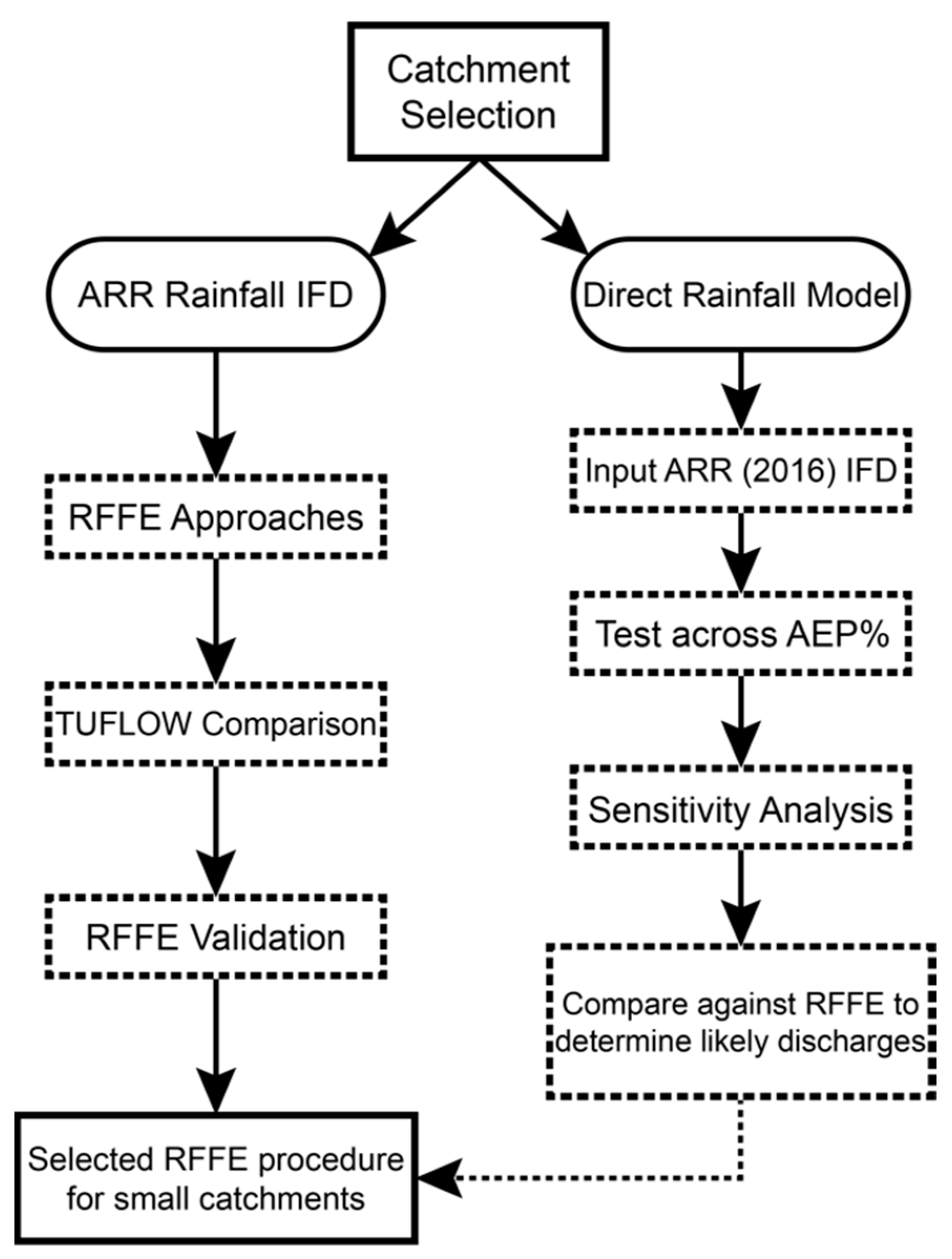
This research tests a series of RFFE methods to calculate predicted peak discharge (Qpeak) previously used within the Pilbara and applies them specifically to smaller sized catchments using updated ARR2019 IFD rainfall values. The selected RFFE methods were chosen based on their satisfactory performance when applied in larger catchments in the Pilbara. The methods tested include a QRT and PRT method from Taylor et al., 2011 [15], QRT and PRT methods from Rahman et al., 2012 [2], a Regional Flood Frequency Procedure (RFFP2000) from Flavell., 2012 [17], a IFM method from Davies and Yip, 2014 [18] and the ARR 2016 RFFE (Table 1). Further details on the RFFE approaches and their prior performance is provided in Table S1 of the Supplementary Material. Next, the RFFE methods are quasi-validated against a TUFLOW direct rainfall model, acting as the observation of rainfall within the catchments lacking gauging infrastructure. The results yield a range of peak discharge estimates for each AEP. The direct rainfall model (and associated sensitivity analysis) is used to provide validation for the most appropriate RFFE for small catchments. Figure 2 shows the full sequence of steps. Similar approaches have been undertaken to assess the performance of ARR 2016 RFFE using RORB modelling [40] or to incorporate it into a direct rainfall model of complex urban catchments [41]. However, few studies have used direct rainfall modelling approaches to benchmark RFFE methods within small semi-arid headwater channels.

3.2. Regionalisation Approaches

Regionalisation refers to the process of transferring hydrological information from one catchment to another. RFFE approaches assume a statistical relationship between observable catchment properties and flood discharge characteristics, allowing the construction of flood hydrographs by applying relationships developed for gauged catchments with similar properties [42]. Regionalization approaches are commonly based either on spatial proximity or similar catchment attributes [43]. Within regionalization methods, model parameters are used as an instrument to transfer hydrological information from gauged to ungauged basins [44]. In general, a regional model can be stated in a simplified form defined by Wagener and Wheater (2006) as:
  θ ^ L = H R θ R ϕ + v R  
where   θ ^ L is the estimated hydrological variable of interest at the ungauged site (it can be an estimated model parameter, probability or cumulative distribution function parameter, or hydrological response such as streamflow or flow events), H R   is a functional relation for   θ ^ L using a set of catchment attributes—physiographic or meteorological attributes ϕ , θ R   is a set of regional hydrological variables of interests and v R is an error term [45]. Regionalisation approaches may be satisfactory if the catchments are similar in some sense, but error prone if they are not [46]. Razavi and Coulibaly (2013) provide a review of methodology for streamflow prediction in ungauged basin using regionalization methods, concluding that most model-dependent methods in arid to warm-temperate climates (e.g., Australia) indicate that physical similarity and spatial proximity appear to be the best approach to estimating streamflow. However, the most regionalisation methods are highly site-specific, and therefore, a comparative study between suitable approaches is suggested before selecting the regionalisation method for a given site or region.

3.3. Regional Flood Frequency Estimation (RFFE)

Regional flood frequency estimation (RFFE) is widely used to estimate flood quartiles in ungauged catchments. RFFE approaches provide an alternative method to flood frequency analysis (FFA) where a lack of temporal data is substituted with spatial data to make more accurate flood estimates at ungauged sites [15]. Common RFFE techniques include Probabilistic Rational Method (PRM), Quantile Regression Techniques (QRT) the Index Flood Method (IFM) and a Parameter Regression Technique (PRT). Regression based RFFE methods are more commonly applied to recent studies within Australia. The following section details selected regression based RFFE methods, which are developed from a longer record of data and are considered to give a more reliable estimation of design flows.

3.3.1. Quartile Regression Technique

The quartile regression technique (QRT) is used frequently within ungauged catchments. The method estimates flood quartiles through a multiple regression between recorded streamflow data and a set of climatic and catchment characteristics within a region [47]. The QRT regression technique is expressed as:
Q T = a B b C C D d
where B, C and D are catchment and climatic characteristics variables (predictors); a, b, c, d are the regression coefficients and Q T is the flood magnitude with T-year ARI (flood quantile) [48].

3.3.2. Parameter Regression Technique

The parameter regression technique (PRT) is similar to the QRT. However, instead of quartiles, the first three moments of the log-Pearson type 3 (LP3) distribution are taken as dependent variables in regression analysis against catchment characteristics [15]. Let Q be the annual maximum flood series at a site and X = ln(Q), then the mean (M), standard deviation (S) and skew (g) of the X series are taken as dependent variables:
ln Q T = M + K T S
where Q T is a flood quantile of T years ARI and K T is the standardized LP3 frequency factor (which is a function of skew) and can be obtained from ARR or can be approximated [15].

3.3.3. Index Flood Method

The index flood method (IFM) assumes that the exceedance probability distribution of annual peak discharge is identical, except for a site-specific scaling factor called the index flood (average likely flood) [49]. The IFM method is expressed as:
Q T = q T μ i
where Q T is the flood quantile, μ i is the function basin area, slope and q T is a regional growth factor (a dimensionless frequency distribution quantity common to all sites within each homogeneous region).

3.4. Australian Rainfall and Runoff (ARR) RFFE

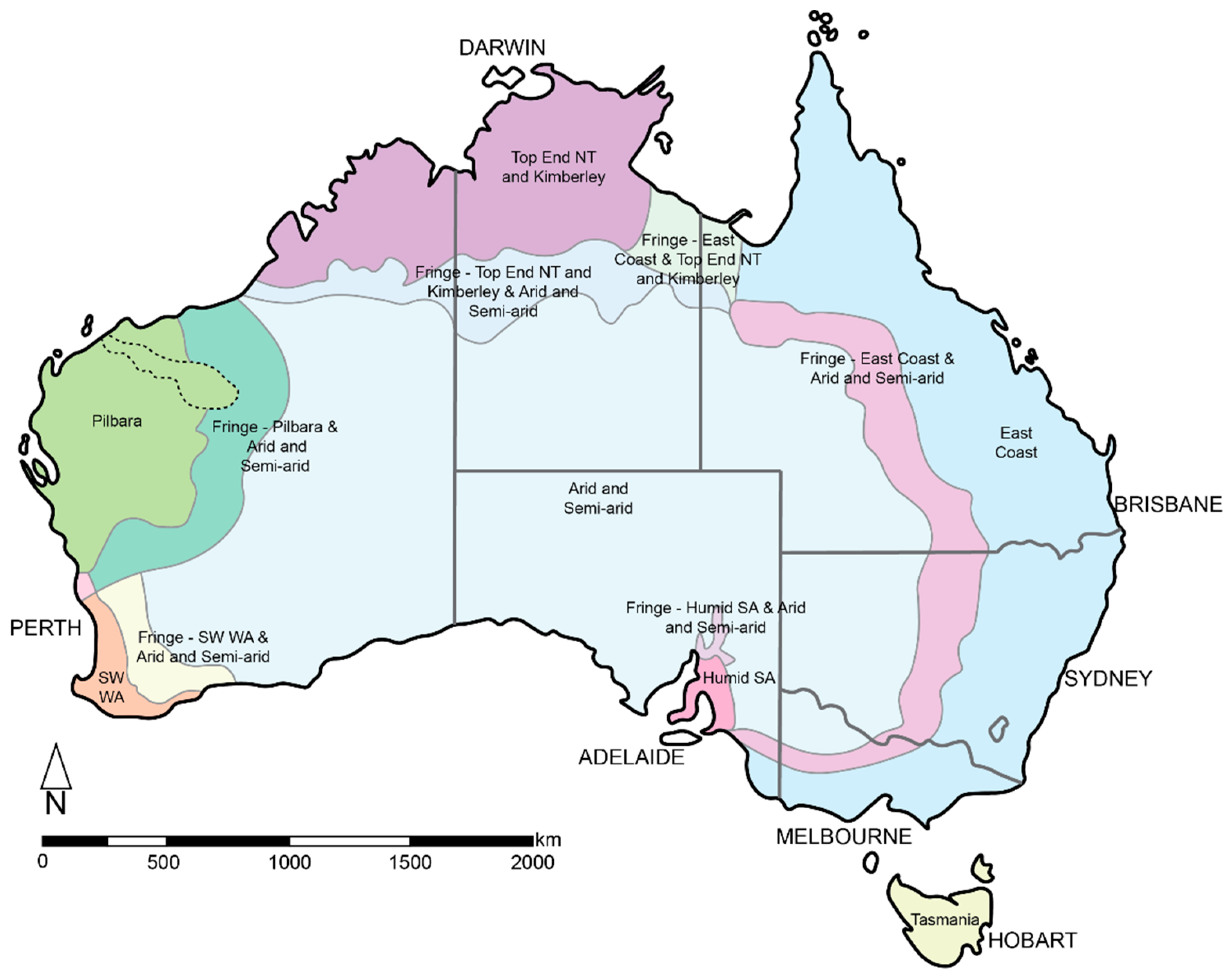
The Australian Rainfall and Runoff (ARR) guidelines offer predicted estimates of rainfall intensity, frequency, and duration (IFD) values for Australia. Additionally, ARR also has a regional flood frequency estimation model which is widely used and recommended for design flood estimation [11,50]. The ARR guidelines were updated in 2016 and again in 2019. Five predictor values were adopted for the RFFE technique [51,52]. These predictor values are: catchment area (in km2); design rainfall intensity at catchment centroid (in mm/h) for the 6 h duration and 50% AEP (50% I6h); design rainfall intensity at catchment centroid (in mm/h) for the 6 h duration and 2% AEP (2% I6h); ratio of design rainfall intensities of AEPs of 2% and 50% for duration of 6 h (2% I6h/50% I6h); and catchment shape factor (Sf), which is defined as the shortest distance between catchment outlet and centroid divided by the square root of catchment area. The RFFE technique used in ARR is adapted for different regions throughout Australia (Figure 3).
Each region is determined based on a Region of Interest (ROI) approach based on geographical proximity of gauging stations, with fringe zones between regions defined by the 500 mm and 400 mm isohyet to delineate between humid and arid/semi-arid regions [53]. The Pilbara region was characterized as an alternative sub-region distinct from the other arid and semi-arid regions of Australia [51]. This was due to (a) concentrations of stream gauging stations in three parts of Western Australia which are separated by long distances (e.g., Kimberley region, Pilbara region and South-West WA) and (b) notable differences in region hydrologic conditions [2]. The approach used for the Pilbara region was modified to an IFM as suggested by Farquharson et al., (1992) [54]. This recommended approach is an IFM with Q10 as an index variable and a dimensionless growth factor (GF) for X% AEP (GFx):
Q x = Q 10 × G F x
A prediction equation was developed for Q10 as a function of catchment characteristics, and regional growth factors were developed based on the estimated at-site flood quartile. A Bayesian parameter estimation procedure with LP3 distribution was used to estimate flood quantiles for each gauged site for AEPs of 50%, 20%, 10%, 5%, 2% and 1%. Rahman et al., (2019) provide further information surrounding this process [52]. The adopted predictive equation for the index variable Q10 has the form:
l o g 10 Q 10 = b 0 + b 1 l o g 10 a r e a + b 2 l o g 10 I 6 ,   50
where b0, b1 and b2 are regression coefficients, estimated using OLS regression, area is the catchment area (in km2) and I6,50 is the design rainfall intensity at catchment centroid for a 6 h duration and 50% AEP. The values of b0, b1 and b2 and the regional growth factors (GFx) are embedded into the RFFE Model 2015.

3.5. Direct Rainfall Modelling

Direct Rainfall Modelling (also known as rain-on-grid) was undertaken in TUFLOW HPC, a 2D fixed-grid, adaptive time-step, hydrodynamic solver that uses an explicit finite volume solution [55]. TUFLOW HPC reduces the run time of models. The direct-rainfall approach applied the rainfall hyetograph (mm versus time) uniformly to active cells within the defined grid of the catchment of interest. Each hyetograph value represents the rainfall that fell per increment. The double precision version of TUFLOW Classic was used in initial model set-up to minimize initial model errors (such as deficient or erroneous data) before running greater numbers of simulations in the GPU for faster run-times after model establishment. TUFLOW Classic uses a fixed time step and will highlight any initial errors with the model runs. Instabilities in the model highlight bad data or poor model set up [56]. TUFLOW HPC can hide poor model set up through its adaptive time-stepping to ensure the model remains stable. Model simulation parameters (grid size, time-step) were established to optimise the accuracy, run-time, and stability of the model. To effectively resolve flow events within the channel it is recommended to provide at least 5 grid/mesh elements laterally across the river channel [57].
The time-step for the model runs was maintained at 1/5 of the selected model grid size in meters (a time-step appropriate for TUFLOW classic) [55] with a cell wet/dry depth of 0.0002 m to account for the high proportion of shallow flow with a direct rainfall model. Due to the small catchment size, rainfall values are small and the reported IL/CL values for larger Pilbara river channels are scaled to these larger catchment hydrological inputs. Simply, the observed losses in larger catchments are larger than the grid-averaged rainfall inputs in small headwater channels. Therefore, IL/CL values were not applied during the final modelled scenarios. Hall (2015) provides a description of the advantages and disadvantages of direct rainfall modelling through model construction, calibration validation and sensitivity analysis [13].

3.5.1. Inputs

Catchment DEMs

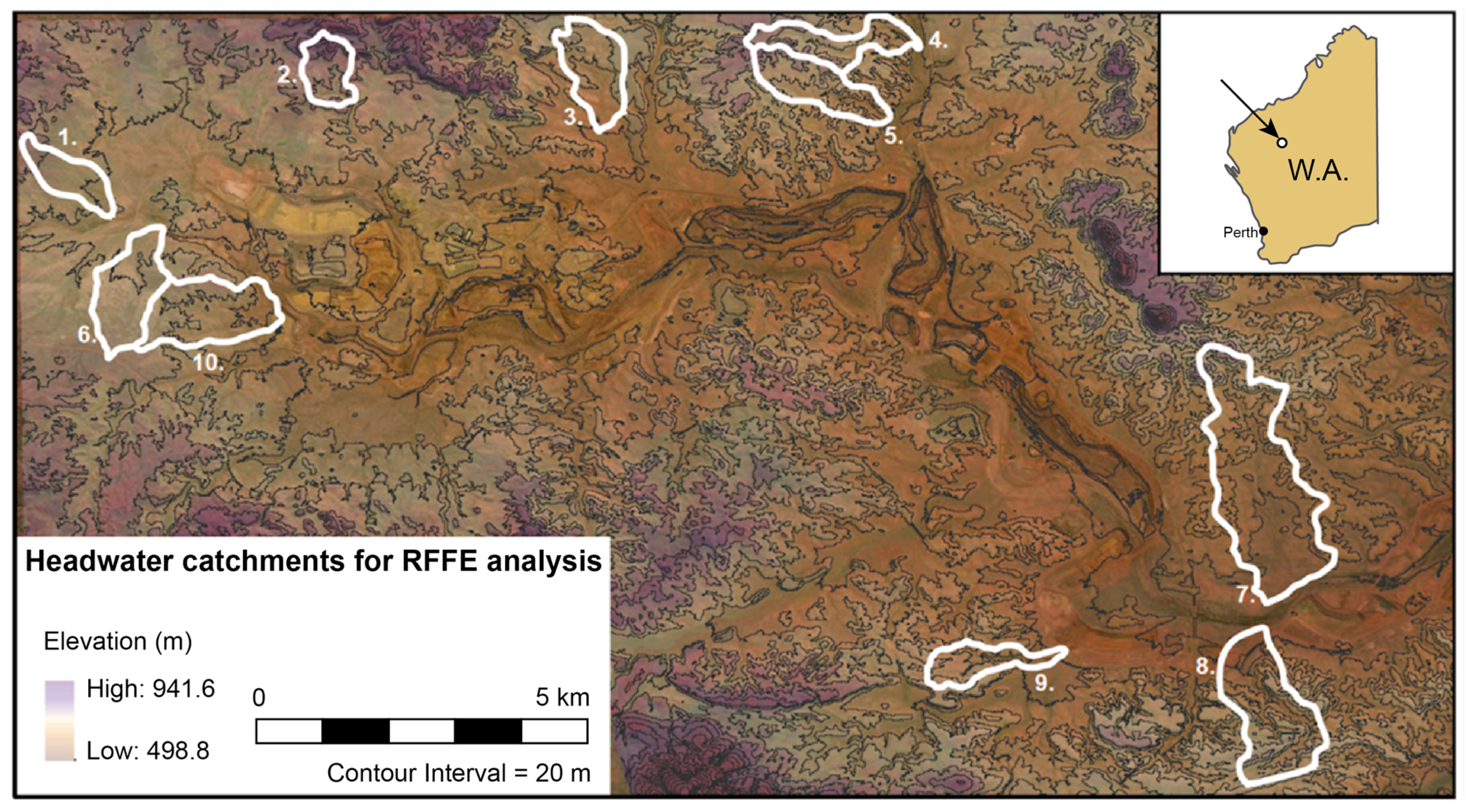
Headwater channels (first-to-third order) are the areas from which water originates within a channel network and are closely coupled to hillslope processes [58]. This study used a high-resolution dataset around the periphery of the Yandi iron ore mine in the Pilbara, WA (Figure 4). Catchments were selected based on the high-resolution dataset covering the full extent of the catchment. Surface catchment DEMs were derived from a wide area semi-global matching (SGM) survey [59] (horizontal accuracy = 0.5 m and vertical accuracy = 0.25 m) undertaken in the Upper Fortescue catchment. Additionally, the catchments were screened for minimal catchment disturbance, such as mining, agriculture of the hydraulic alteration of the waterway from bridges and culverts. Catchments with engineering infrastructure, such as railways, culverts and main roads were modelled until the upstream contact with these features. Ten catchments (ranging from 0.96 km2 to 9.23 km2) matched these requirements and were selected to test the RFFE approaches (Table 2).

Rainfall

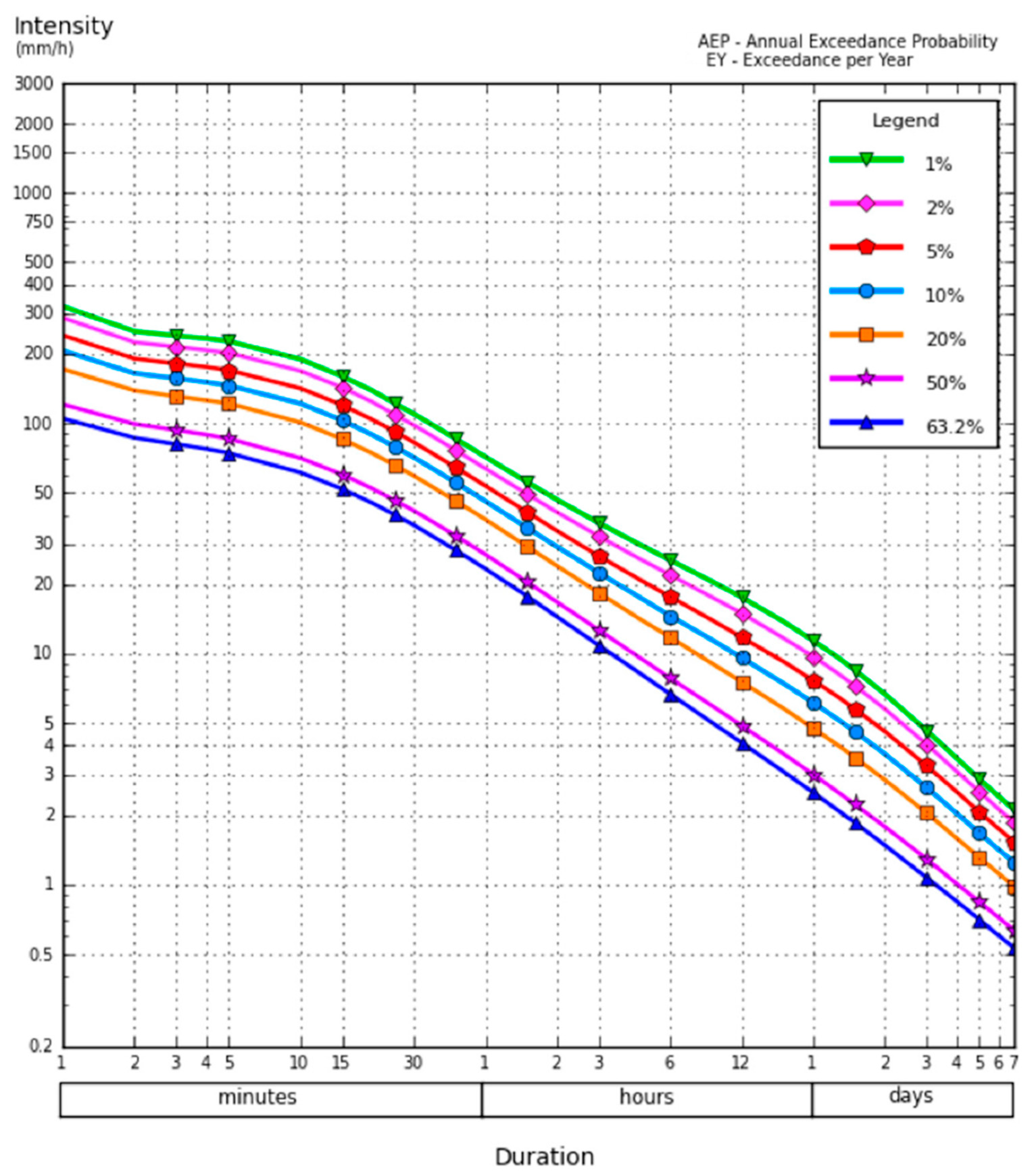
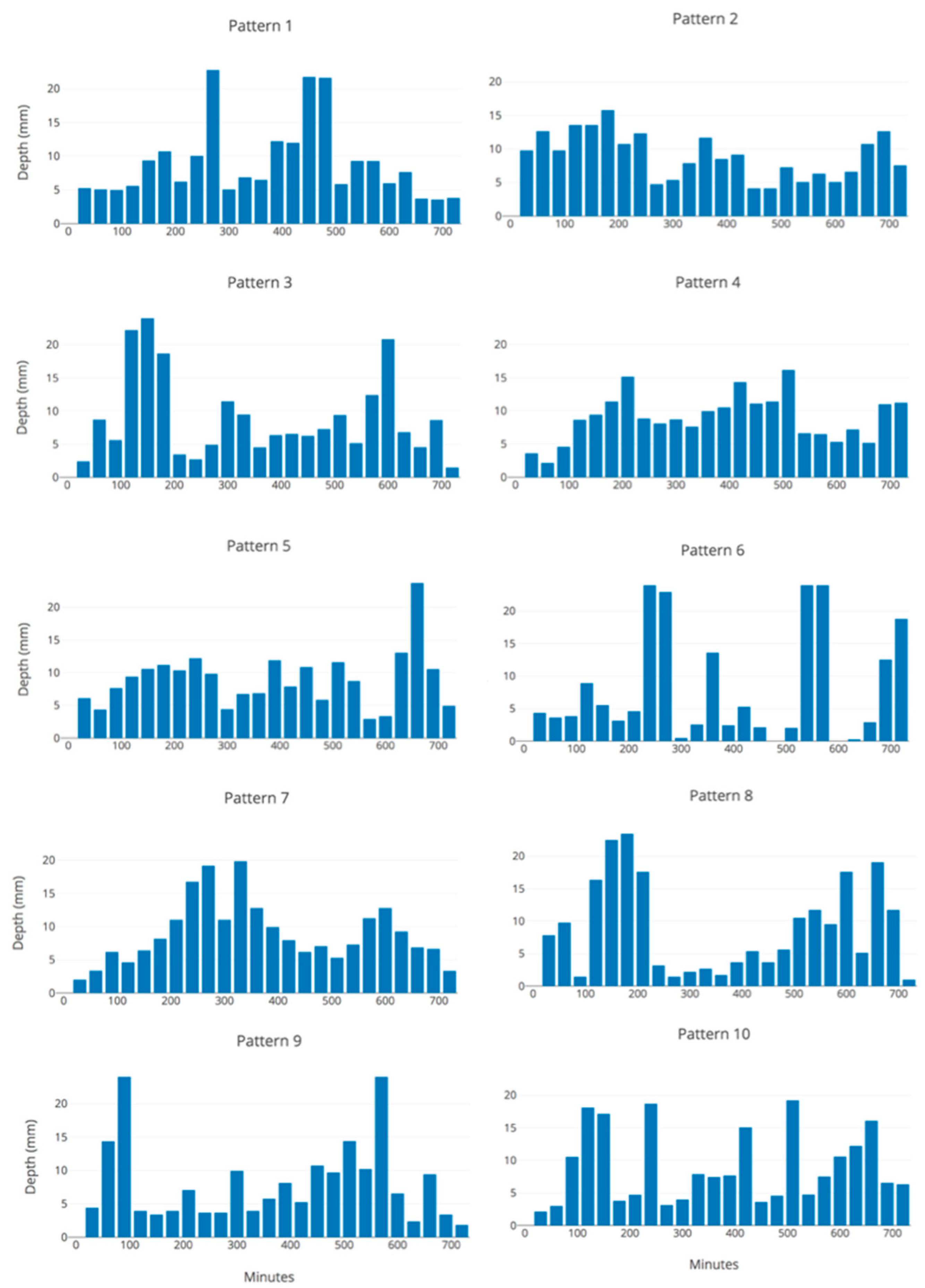
The Bureau of Meteorology, Australia (BOM) 2016 Design Rainfall Data System [60] was used to provide rainfall intensities for RFFE analysis and as a modelling input for direct rainfall modelling. The BOM 2016 IFD values provide a rainfall intensity (mm/h) or depth (mm) based on the latitude, longitude, and catchment size within a set location (Figure 5). BOM2016 IFD values replaced the older 1987 IFD and interim 2013 IFD values providing 30 additional years of hydrological data and adjustments to the approach. Additionally, the direct rainfall was applied to the 2D model over the entire catchment as time-series data as mm versus hours. The time-series data has a histogram stair-step shape) therefore rainfall was applied as a stepped approach holding the rainfall constant during the allocated time interval (BMT, 2018) meaning each rainfall value is the amount of rain that fell in mm between the previous time and current time. Rainfall was applied to every active cell within the digitised catchment. Ten varied areal hyetograph patterns were used for each catchment (Figure 6). Podger et al., (2018) provide a detailed description of the creation of these hyetograph patterns [61].

3.5.2. Roughness

Manning’s n values were assigned to account for runoff conditions. The roughness values assigned within a direct rainfall model can affect the timing of runoff. Additionally, constant roughness values may underestimate the effective roughness and ignores the role of spatially varied roughness within the catchment. Catchment floodplains were assigned a Manning’s value of n = 0.02 and the channel was assigned a default Manning’s value of 0.035. Adjustments of the roughness values were made in the sensitivity analysis of the TUFLOW models.

3.5.3. Output

Discharge

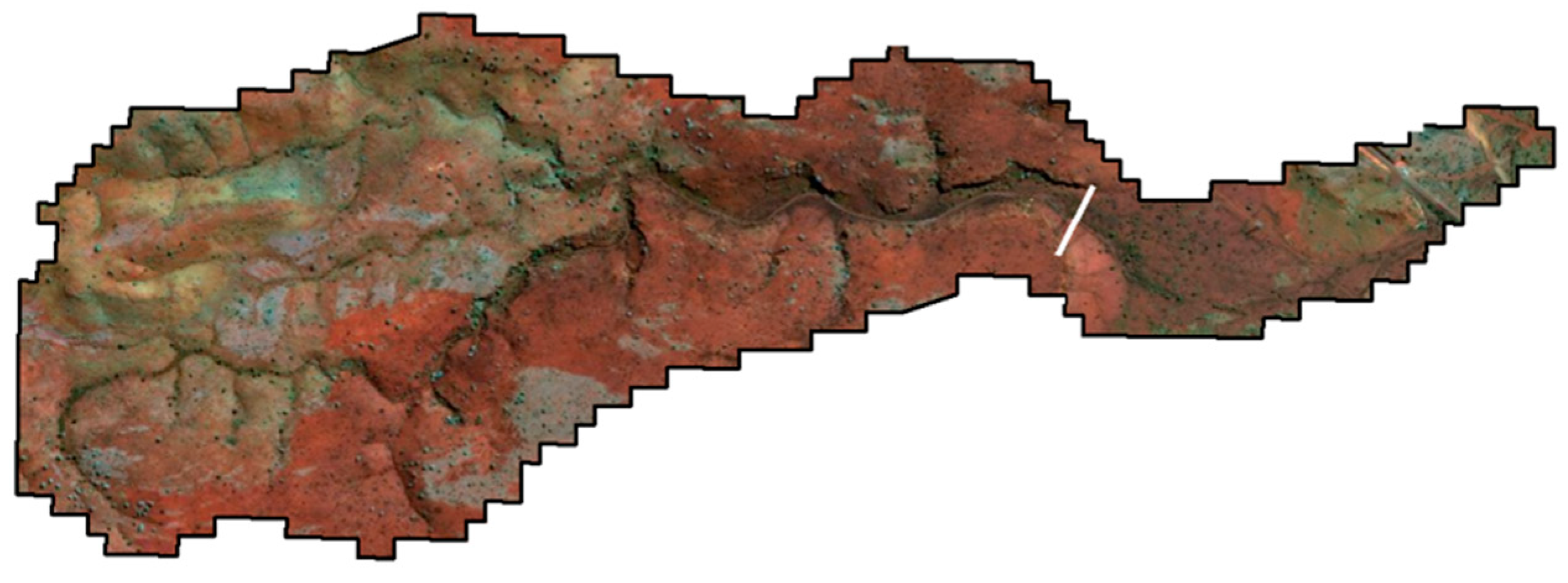
For each catchment a cross section was delineated near the catchment outlet, (Figure 7). At this cross section, a plot output was created in the form of a time-series hydrograph. This time-series provides the flood flow through the catchment during each model scenario and is used to identify peak discharge (Qpeak) values for each rainfall event. Backwater development has been reported during flood modelling of channel confluences within the larger Marillana Catchment [62]. Therefore, cross sections were delineated slightly upstream from the catchment outlet to reduce backwater flow events impacting peak discharge values during flood modelling.
In addition to using the plot output for each simulation, maps of water depth (d) and velocity (V) were constructed at each of the model time-steps. The output from this was used to make an independent estimate of discharge using a velocity-area method:
Q = AV
where Q is the discharge expressed in cubic meters per second (m3 s−1 or cumecs), A is the stream cross sectional area (m2) and V is the mean velocity of stream flow (m s−1). Measurements of stream water depth (stage) are typically measured at sites within the Pilbara, however continuous flow measurement of river discharge is expensive and logistically unwise given the annual frequency of flow events within the region.

3.6. Sensitivity Analysis

Sensitivity analysis or calibration methods are critical steps in rainfall-runoff and developing useful models of complicated hydrologic systems [63,64]. Models can be calibrated to observed data to demonstrate that the model can produce an observed flow time series with an acceptable level of accuracy [64]. Alternatively, a model may be available that has been previously calibrated for a catchment as part of another study. Sensitive model parameters should be recognised and appropriately evaluated to ensure they are constrained within acceptable ranges. Prediction in ungauged basins is challenging to validate owing to the data limitations within the area. When models are not able to be calibrated to measurements sensitivity testing should at least be carried out to assess the sensitivity of the model to variations in the main model parameters [11]. Model evaluation may not be limited to how accurately model predictions match historical observations, but how well the model represents the hydrological system. In this paper, we use a direct rainfall model to quasi-validate and select the most appropriate RFFE procedure for headwater, small size catchments. All RFFE procedures used in this investigation have been previously calibrated on larger catchments in the Pilbara.
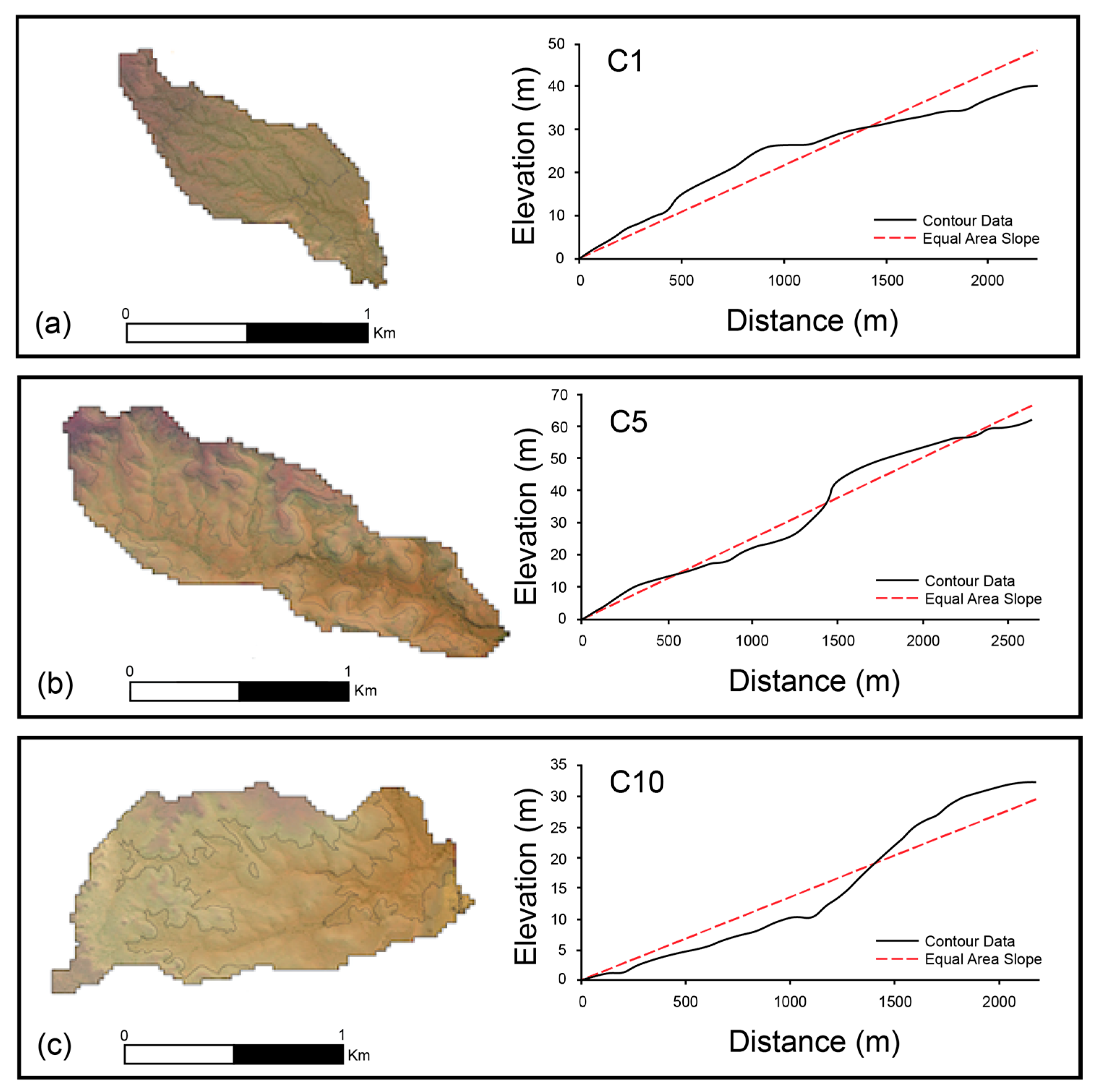
There is no standard method for estimating uncertainty in streamflow in ungauged basins using regionalisation techniques [44]. Uncertainty is estimated here in the sensitivity analysis of the direct rainfall modelling approach by adjusting model parameters on three catchments. (Figure 8). Sensitivity analysis was carried out to determine the optimum model running conditions and explore the suitability of direct rainfall modelling within these small headwater catchments. Catchments were selected on the basis of channel gradient to encompass a range of catchment types within the analysis. Catchment 5 was the steepest, with greater expected areas of supercritical flow and areas of complex terrain which would challenge model performance [56]. Other catchments included catchment 1; a small, shallow, unconfined channel with multiple flow paths and 10; a larger catchment with a predominantly unconfined single-thread channel representative of many of the headwater channels in the vicinity.
Existing direct rainfall models have been found to be most sensitive to Manning’s roughness and rainfall [13] and therefore sensitivity analysis was carried out to address the parameters that have larger uncertainties within the model. Sensitivity analysis was carried out to address: rainfall hyetograph shape, Manning’s roughness (adjusted to +/− 20% or the upper and lower bounds for characteristic minor natural streams [65] and grid sizing, assessed with a 1 m, 2 m, 5 m and 10 m spacing.

3.7. Procedure for Evaluating RFFE Approaches

To evaluate the RFFE approaches, we use the result of the direct rainfall model to act as a measured series in this “quasi-validation”. This quasi-validation uses joint plots of the RFFE output and simulated rain-on-grid discharge to compare the output of predictive methods. The ARR RFFE approach provides confidence limits of 5% Lower confidence limit (LCL) and a 95% Upper confidence limit (UCL) which are used as the absolute cut off for RFFE values. The evaluation procedure was as follows: (1) Was the RFFE output within the 5–95% confidence limit range for the ARR approach? (2) Did the approach demonstrate appropriate hydrological scaling across space and flood return period? (i.e., did the results increase with an increase in rainfall magnitude or catchment area) and lastly, (3) Did RFFE results display good agreement with findings from the rain-on-grid model? If not, did any approaches align with other tested RFFE methods.

4. Results

4.1. Estimates of Peak Discharge for RFFE Methods

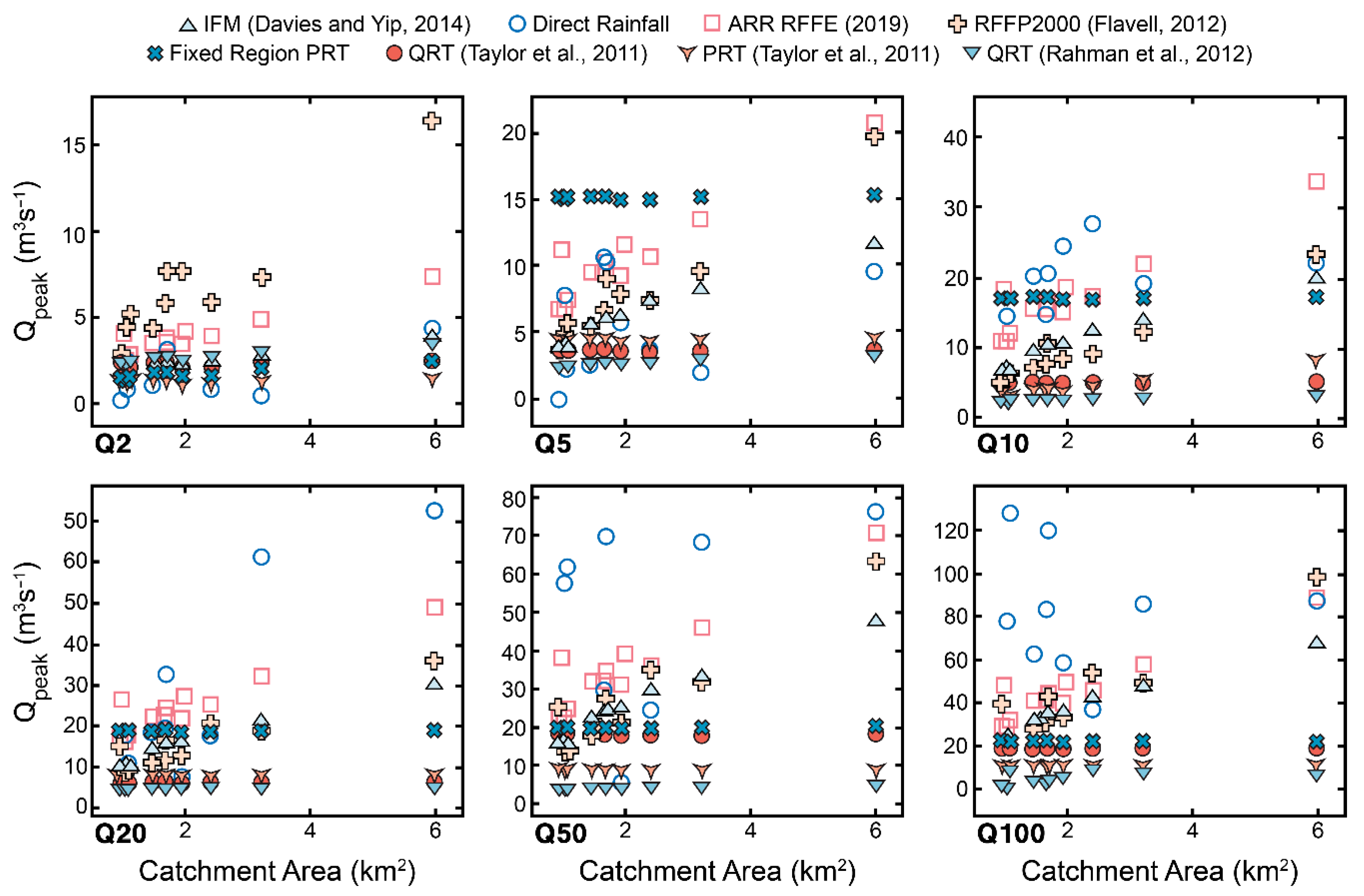
Rainfall values for RFFE approaches were obtained from BOM Design Rainfall Data System (2016) using 2016 Intensity, Frequency and Duration (IFD) values. The rainfall output showed a relatively homogenous depth for catchments ranging between 0.96 km2 and 2 km2. Larger catchments (sized 5.99 and 3.23 km2) were predicted to have higher rainfall depths for the 12 h storm across the range of AEP (Table 3). A wide range of Qpp values were obtained using the RFFE equations (Figure 9). The Flavell RFFP2000 procedure produced higher Qpp values for Q2 events. Between Q5 and Q100, the ARR values were highest, with greatest agreement with the IFM and Flavell RFFP2000. The PRT and QRT approach from Taylor et al., (2011) show nearly identical values with no increase in peak discharge values for an increase in catchment size. The fixed region PRT (Rahman et al., 2012) provided the lowest estimates of predicted peak discharge. Both QRT and PRT approaches produced low discharge values across Q10–Q100 flow events.

4.2. Direct Rainfall Catchment Modelling

Table 4 shows the output values from direct rainfall modelling from the 10 catchments. Figure 10 show the results of direct rainfall modelling. These values have also been plotted next to the RFFE approaches with similar output (ARR RFFE (2019), IFM (Davies and Yip, 2014) and the Flavell RFFP (Flavell, (2012)) selected from deductive reasoning, omitting PRT and QRT approaches that yielded uncharacteristically small flood magnitudes across all annual exceedance probability.

4.3. TUFLOW Sensitivity Analysis

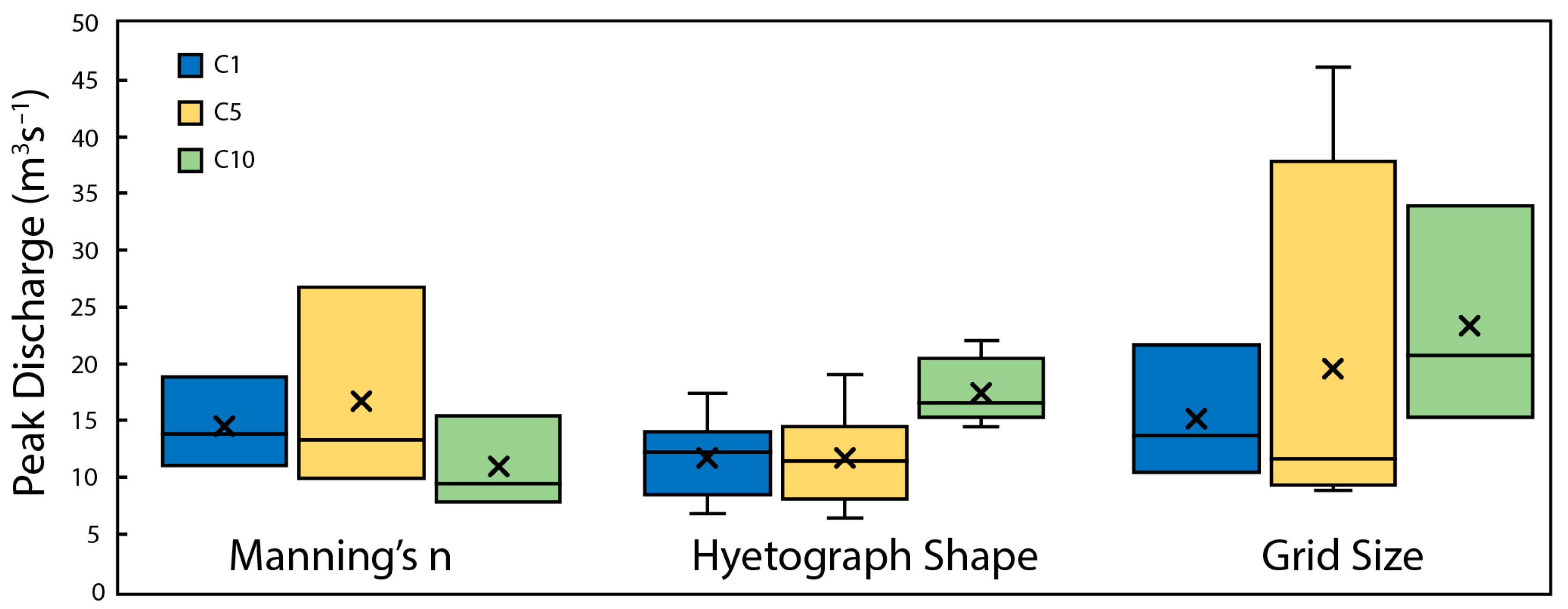
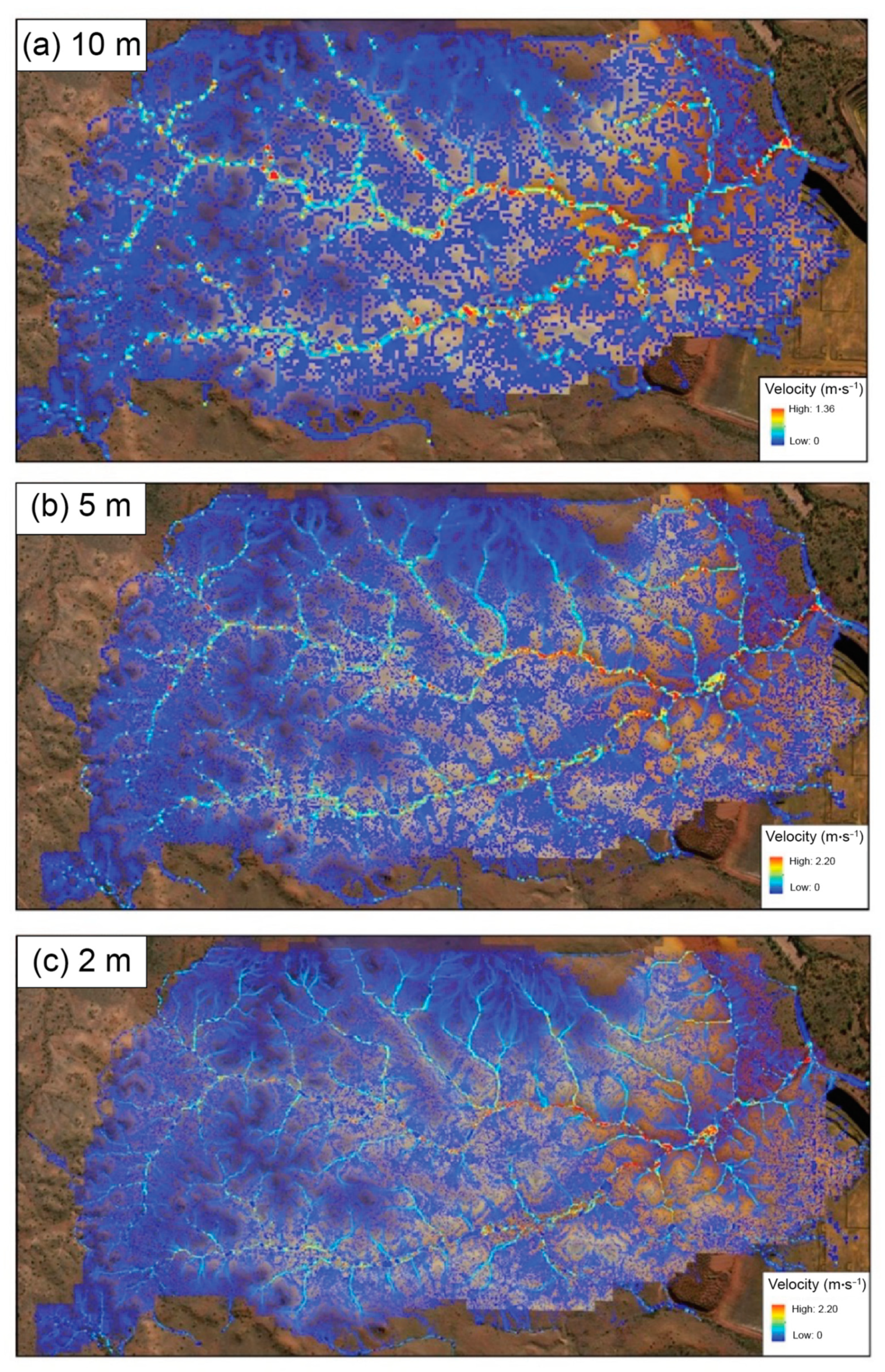
The results of the sensitivity analysis are found in Figure 11. The grid size of the model caused large variability in peak discharge values. Changes in peak velocity values were sensitive to this change in grid size, resulting in higher velocities (as one would expect) for a higher resolution DEM (e.g., 2 m) compared to the 10 m grid size. This increase in velocity is attributed to the more detailed topographic representation of channel constrictions and channel bed heterogeneity in the higher resolution grid size (Figure 12). C5 was the steepest and most topographically varied catchment, with steep confining areas. Within this catchment there was greater variability in the peak discharge from adjustments to Manning’s n value, hyetograph shape, (and most prominently) grid size; where Qpp values were doubled between a grid size increment increase of 5 m to 10 m. Final model scenarios used a grid size of 2 m, rainfall pattern 6, which resulted in the highest peak discharge in sensitivity analysis and a channel-wide Manning’s roughness value of 0.035. The range of output values for the sensitivity analysis are found in Table 5.

5. Discussion

5.1. Direct Rainfall Model Performance

5.1.1. Sensitivity Analysis

Sensitivity analysis of the direct rainfall model has indicated that the steeper, confined C5 is more sensitive to alterations in grid size, Manning’s n and hyetograph shape. Further research and integration of IL/CL values would improve the model’s representation of headwater channel processes. A grid size of 2 m was selected to avoid excessive computation time but to integrate detailed topographic forms such as smaller flowpaths and to capture the heterogeneity of the natural environment. Higher within a catchment, flowpaths become smaller and may be poorly represented by the model if they exist on a sub-grid scale, affecting the timing of runoff routing within the catchment [57] (ARR, 2012). This is likely a key contributor to the increased Qpp values for coarser resolution model grid sizes (5–10 m). Mesh (grid-size) resolution has been shown to have a high impact on a models output flow volume in other studies conducting direct rainfall in small catchments [23]. Additionally, the slope between neighbouring cells has a key influence on the behaviour of catchment runoff, and therefore peak discharge values. Care should be taken to adequately understand the potential variability in peak discharge estimation using direct rainfall models. Additionally, explicit consideration of local variation in rainfall patterns in peak flood discharge modelling efforts is advised.

5.1.2. Applicability of Direct Rainfall Modelling in Headwater Catchments

Direct rainfall models are subject to higher levels of mass error when using the direct rainfall approach particularly where the model has areas of steep, complex flow or the model is located at a high elevation above sea level and experience relatively small inflows [56]. The catchments modelled here have many of these challenges. They are small catchments with small inflows, and experience sudden changes in slope conditions. Drainage pathways are not clearly defined and for some catchments, the hydrological boundaries between channel and floodplain are difficult to model. Flow is routed along the floodplain or within a claypan environment culminating in diffusive and complex drainage patterns. For these catchments, there were unexpected peak discharge values which may not fully represent what would occur in these catchments outside of where flow is rapidly dispersed away from channel setting (e.g., catchment 10).
The catchment outlet of several small headwater channels was prone to backwater effects. Such backwater effects have been reported for other channels in the Pilbara region from constrictions within the channel [34]. Backwaters can decrease velocities, raise the water surface elevation (WSE) and extend upstream [34]. Peak discharge values obtained from the catchment outlet were based on a cross section beyond the extent of backwater effects from outlet constrictions or tributary junctions. Care was taken to inspect the mapped output to interpret the water surface elevation at catchment cross sections.
Despite these warnings, the use of direct rainfall modelling is useful within small catchments with well-defined drainage pathways to quasi-calibrate selected RFFE approaches in the complete absence of rainfall and streamflow data. In doing so, an approximation of likely flood flows within these ungauged settings can be made. However, direct rainfall modelling with these catchment characteristics should not replace a hydrologic modellers perspicacity in dealing with flow estimation within dryland headwater environments. Even when calibration is properly done, models tend to have greater predictive strengths over shorter timeframes than longer timeframes as the system over short time scales is more similar to the one which it was calibrated for. Therefore, greater trust can be placed on the more frequent flow predictions than longterm flow dynamics within these headwater catchments.

5.2. RFFE Evaluation

The evaluation procedure was as follows: (1) Was the RFFE output within the 5–95% confidence limit range for the ARR approach. (2) Did the approach demonstrate appropriate hydrological scaling across space and flood return period (i.e., did the results increase with an increase in rainfall magnitude or catchment area) and lastly, (3) Did RFFE results display good agreement with findings from the rain-on-grid model and if not, did any approaches align with other tested RFFE methods. Many of the RFFE approaches for the Pilbara region are created using far larger catchment sizes. For example, the Flavell RFFP2000 approach is derived from an average catchment size of 5570 km2 and this research tests the application of this RFFE in catchments with an average size of 2.16 km2. Despite this magnitude variation in catchment size, these RFFE approaches are used in these smaller catchments for design discharge calculations. However, the direct modelling highlights that catchment representativeness remains an issue. This issue is exacerbated by sparse gauging coverage and continues to be a high priority for future research [57].
The RFFP2000 (Flavell, 2012), IFM (Davies and Yip, 2014) and ARR RFFE (2019) methods produce higher estimates of peak discharge. These three methods diverge from the other approaches in estimating higher peak discharge estimates and this deviation is more pronounced in less frequent flood flows (Q20, Q50 and Q100). These three methods are also more sensitive to changes in catchment area with larger catchments (above 5 km2) predicted to have peak discharges double that of smaller catchments (around 2 km2).
Both PRT methods estimate the lowest peak discharge values across all ARI, with little increase in discharge across less frequent flood flow events. These estimation techniques are less sensitive to catchment size and may overlook flood flow magnitudes within smaller catchments as they were created with a dataset comprised of larger catchments. Additionally, parameter regression techniques give emphasis to the mean and therefore frequent flows [66]. These methods provide a lower estimate of peak discharges, with emphasis on frequent flow events and are likely not suited to smaller headwater catchments such as those in this study.
The QRT methods show slightly higher predicted peak discharges but still do not provide convincing flood discharges at higher return intervals. PRT and QRT methods should be used with caution on smaller headwater channels. The IFM (Davies and Yip, 2014) method uses greater weighted frequency factors which results in the larger range of peak flood values across return intervals. This greater range of frequency factors for the IFM method compared to the PRT methods is likely to better represent higher magnitude flow events within these headwater catchments.
The ARR RFFE (2019) [25] approach is industry standard for larger catchments and is useful for small headwater catchments even if it is likely to provide a conservative estimate. The ARR RFFE model is noted to have large uncertainty with mean relative errors of 50–60% [57]. Alternative methods developed by Flavell (RFFP2000 and RFFP2006) and by Davies and Yip (2014) have been suggested as viable locally developed replacements to ARR2015 methods for the Pilbara region [57]. The Flavell RFFE approach is relatively complicated in comparison to the IFM and ARR (RFFE) 2019 approaches. The Flavell RFFP approach requires some catchment analysis to provide equation values (such as slope, latitude, longitude, length of catchment) but it is likely these values would be easy to populate for any catchment of interest. The Davies and Yip (2014) IFM approach uses a wide spatial distribution and catchment range in developing design equations making it applicable throughout the Indian Ocean drainage division [18]. The RFFP2000, IFM and ARR RFFE (2019) are therefore suggested for the estimate of peak discharge values within small ungauged headwater channels.

6. Conclusions

The role of this research was to identify peak discharge values from a direct rainfall model, and to compare these findings with RFFE approaches conducted within the region. Within the TUFLOW direct rainfall model simulations, the model was predominantly sensitive to grid size and Manning’s n, with the rainfall pattern having a smaller impact on Qpeak. It is worth noting however that even the variation in the shape of the hyetograph produced up to 50% variation in the final Qpeak value within the sensitivity analysis. Therefore, awareness of the limitations of direct rainfall modelling within these steeper catchments is necessary when using this approach or selecting an RFFE approach. Despite this caution, the Flavell RFFP2000 and Davies and Yip, (2014) IFM appear the most reasonable estimates of peak discharge within the channels. These approaches provide lower estimates than the ARR2019 RFFE models, which are suggested to provide higher flow rates and are commonly used as part of a conservative approach to waterway design within the Pilbara. Whilst the direct rainfall modelling approach has many barriers when applied to headwater channels, this approach is useful to provide a frame of reference when selecting an RFFE approach for ungauged headwater catchments. It is common for a RFFE approach to be applied without first considering the weaknesses and limitations of the derived equation, or its suitability within small headwater catchments. Here, we show the potential for direct rainfall modelling and its applicability in an environment with limited opportunities to validate peak flood discharge estimation methods. The lack of gauged real-world measurements within these catchments continues to present the main obstacle in improving our understanding of flow conditions and rainfall values within the Pilbara region.

Supplementary Materials

The following supporting information can be downloaded at: https://www.mdpi.com/article/10.3390/hydrology9100165/s1, Table S1: Supplementary material highlighting key method details for the RFFE estimation methods applied to headwater catchments in the Pilbara, WA.

Author Contributions

Conceptualization, A.F. and I.R.; methodology, A.F. and I.R.; software, A.F., writing—original draft preparation, A.F.; writing—review and editing, A.F. and I.R. All authors have read and agreed to the published version of the manuscript.

Funding

This research was funded the University of Melbourne Research Scholarship with additional funding from BHP, Australia (Project 041639).

Data Availability Statement

Data available on request from the authors.

Acknowledgments

The authors would like to thank the 3RG research group for their discussions surrounding this work. We would also like to acknowledge the support of Iain Rea of BHP for this research.

Conflicts of Interest

The authors declare no conflict of interest.

References

  1. Hailegeorgis, T.T.; Alfredsen, K. Regional flood frequency analysis and prediction in ungauged basins including estimation of major uncertainties for mid-Norway. J. Hydrol. Reg. Stud. 2017, 9, 104–126. [Google Scholar] [CrossRef]
  2. Rahman, A.; Haddad, K.; Zaman, M.; Ishak, E.; Kuczera, G.; Weinmann, E. Australian Rainfall and Runoff Revision Project 5: Regional Flood Methods: Stage 2 Report. P5/S2/015. 2012. Available online: http://www.arr.org.au/wp-content/uploads/2013/Projects/ARR_Project5_Stage2_Report_Final_.pdf (accessed on 24 August 2022).
  3. Feldman, A.D. Flood Hydrograph and Peak Flow Frequency Analysis; US Army Corps of Engineers: Davis, CA, USA, 1979.
  4. Canterford, R.P.; Pescod, N.R.; Pearce, N.H.; Turner, L.H.; Atkinson, R.J. Frequency analysis of Australian rainfall data as used for flood analysis and design. In Regional Flood Frequency Analysis: Proceedings of the International Symposium on Flood Frequency and Risk Analyses, Baton Rouge, LA, USA, 14–17 May 1987; Springer: Dordrecht, The Netherlands, 1987; pp. 293–302. [Google Scholar]
  5. Ladson, A.R.; Weinmann, E. Hydrology—An Australian Introduction. Australas. J. Water Resour. 2008, 12, 71–72. [Google Scholar] [CrossRef]
  6. Pilgrim, D.H.; Chapman, T.G.; Doran, D.G. Problems of rainfall-runoff modelling in arid and semi-arid regions. Hydrol. Sci. J. 1988, 33, 379400. [Google Scholar] [CrossRef]
  7. Chamber of Minerals and Energy of Western Australia (CME). Iron Ore. 2022. Available online: https://www.cmewa.com.au/about/wa-resources/iron-ore/ (accessed on 24 August 2022).
  8. Refsgaard, J.C.; Knudsen, J. Operational Validation and Intercomparison of Different Types of Hydrological Models. Water Resour. Res. 1996, 32, 2189–2202. [Google Scholar] [CrossRef]
  9. Flatley, A.; Markham, A. Establishing effective mine closure criteria for river diversion channels. J. Environ. Manag. 2021, 287, 112287. [Google Scholar] [CrossRef]
  10. Huxley, C.; Syme, B. TUFLOW GPU-best practice advice for hydrologic and hydraulic model simulations. In Proceedings of the 37th Hydrology & Water Resources Symposium, Queenstown, New Zealand, 28 November–2 December 2016; pp. 195–203. [Google Scholar]
  11. Ball, J.E.; Babister, M.K.; Nathan, R.; Weinmann, P.E.; Weeks, W.; Retallick, M.; Testoni, I. Australian Rainfall and Runoff—A Guide to Flood Estimation; Institution of Engineers: Barton, Australia, 2016. [Google Scholar]
  12. Caddis, B.M.; Jempson, M.A.; Ball, J.E.; Syme, W.J. Incorporating hydrology into 2D hydraulic models–the direct rainfall approach. In Proceedings of the 9th National Conference on Hydraulics in Water Engineering, Darwin, Australia, 23–26 September 2008. [Google Scholar]
  13. Hall, J. Direct rainfall flood modelling: The good, the bad and the ugly. Aust. J. Water Resour. 2015, 19, 74–85. [Google Scholar] [CrossRef]
  14. Taylor, H.; Kerr, T. Designing for Mining: Challenges of Hydrological Design in the Pilbara. Hydrol. Water Resour. Symp. 2014, 2014, 4452. [Google Scholar]
  15. Taylor, M.; Haddad, K.; Zaman, M.; Rahman, A. Regional flood modelling in Western Australia: Application of regression-based methods using ordinary least squares. In Proceedings of the 19th International Congress on Modelling and Simulation, Perth, Australia, 12–16 December 2011; pp. 3803–3810. [Google Scholar]
  16. Rahman, A.; Zaman, M.; Haddad, K.; Kuczera, G.; Weinmann, E.; Weeks, W.; Rajaratnam, L.; Kemp, D. Development of a new regional flood frequency analysis method for semi-arid and arid regions of Australia. In Proceedings of the 34th Hydrology and Water Resources Symposium Sydney, Sydney, Australia, 19–22 November 2012; pp. 1433–1440. [Google Scholar]
  17. Flavell, D. Design flood estimation in Western Australia. Australas. J. Water Resour. 2012, 16, 1–20. [Google Scholar] [CrossRef]
  18. Davies, J.R.; Yip, E. Pilbara Regional Flood Frequency Analysis. In Proceedings of the Hydrology and Water Resources Symposium, Perth, Australia, 24–27 February 2014; pp. 182–189. [Google Scholar]
  19. Oreskes, N.; Shrader-Frechette, K.; Belitz, K. Verification, validation, and confirmation of numerical models in the earth sciences. Science 1994, 263, 641–646. [Google Scholar] [CrossRef] [PubMed]
  20. Annis, A.; Nardi, F.; Volpi, E.; Fiori, A. Quantifying the relative impact of hydrological and hydraulic modelling parameterizations on uncertainty of inundation maps. Hydrol. Sci. J. 2020, 65, 507–523. [Google Scholar] [CrossRef]
  21. Ahmadisharaf, E.; Kalyanapu, A.J.; Bates, P.D. A probabilistic framework for floodplain mapping using hydrological modeling and unsteady hydraulic modeling. Hydrol. Sci. J. 2018, 63, 1759–1775. [Google Scholar] [CrossRef]
  22. Grillakis, M.G.; Koutroulis, A.G.; Komma, J.; Tsanis, I.K.; Wagner, W.; Blöschl, G. Initial soil moisture effects on flash flood generation—A comparison between basins of contrasting hydro-climatic conditions. J. Hydrol. 2016, 541, 206–217. [Google Scholar] [CrossRef]
  23. David, A.; Schmalz, B. Flood hazard analysis in small catchments: Comparison of hydrological and hydrodynamic approaches by the use of direct rainfall. J. Flood Risk Manag. 2020, 13, e12639. [Google Scholar] [CrossRef]
  24. Viglione, A.; Blösch, G. On the role of storm duration in the mapping of rainfall to flood return periods. Hydrol. Earth Syst. Sci. 2009, 13, 205–216. [Google Scholar] [CrossRef]
  25. Ball, J.; Babister, M.; Nathan, R.; Weeks, W.; Weinmann, E.; Retallick, M.; Testoni, I. (Eds.) Australian Rainfall and Runoff: A Guide to Flood Estimation; Geoscience Australia: Canberra, Australia, 2019. [Google Scholar]
  26. Ruprecht, J. Arid Zone Hydrology: Pilbara region of Western Australia. In Proceedings of the 23rd Hydrology and Water Resources Symposium, Hobart, Australia, 21–24 May 1996; pp. 301–305. [Google Scholar]
  27. Broit, A.; Boytar, G. Development of a methodology for catchments exhibiting sheet flow characteristics in the Pilbara region. Hydrol. Water Resour. Symp. 2014, 2014, 953–961. [Google Scholar]
  28. BHP Billiton Iron Ore Pty Ltd. BHP Billiton Iron Ore Pilbara Expansion: Strategic Proposal, 650 Environmental Scoping Document. November 2013. Available online: https://www.bhp.com/-/media/bhp/regulatory-information-media/iron-ore/western-australia-iron-ore/0000/referral-and-environmental-scoping-document/160316_ironore_waio_pilbarastrategicassessment_state_environmentalscopingdocument.pdf (accessed on 24 August 2022).
  29. Peel, M.C.; Finlayson, B.L.; McMahon, T.A. Updated world map of the Köppen Geiger climate classification. Hydrol. Earth Syst. Sci. 2007, 11, 1633–1644. [Google Scholar] [CrossRef]
  30. Sudmeyer, R. Climate in the Pilbara. Bulletin 4873, Department of Agriculture and Food, Western Australia, Perth. Available online: https://library.dpird.wa.gov.au/bulletins/220/ (accessed on 24 August 2022).
  31. Charles, S.P.; Fu, G.; Silberstein, R.P.; Mpelasoka, F.; McFarlane, D.; Hodgson, G.; Teng, J.; Gabrovsek, C.; Ali, R.; Barron, O.; et al. Hydroclimate of the Pilbara: Past, Present, and Future. A Report to the Government of Western Australia and Industry Partners from the CSIRO Pilbara Water Resource Assessment; CSIRO Land and Water: Clayton, Australia, 2015; pp. 1–140. [Google Scholar]
  32. Ruprecht, J.; Ivansecu, S. Surface Hydrology of the Pilbara Region: Summary Report. Surface Water Hydrology Report; Series no. 32; Water and Rivers Commission: Perth, Australia, 2000. [Google Scholar]
  33. Wark, B.; Thomas, L. Does your rating curve hold water: The consequence of rating 860 curve errors. In Proceedings of the ANCOLD, Canberra, Australia, 21–22 October 2014; pp. 1–11. [Google Scholar]
  34. Harvey, M.; Pearcey, M.; Price, K.; Devkota, B. Geomorphic, hydraulic and sediment transport modelling for mine related channel realignment—Case Study: Caves Creek, Pilbara, Western Australia. In Hydrology and Water Resources Symposium; Engineers Australia: Queensland, Australia, 2014; pp. 259–266. [Google Scholar]
  35. MWH. Ecohydrological Conceptualisation of the Fortescue Marsh Region; Project No. 83501069; MWH: Melbourne, Australia, 2015; pp. 1–178. [Google Scholar]
  36. Bureau of Meterology (Australia). Tropical Cyclone Climatology Maps. Product Code: IDCJCM0011. 2019. Available online: http://www.bom.gov.au/climate/maps/averages/tropical-cyclones/ (accessed on 24 August 2022).
  37. Haque, M.M.; Rahman, A.; Haddad, K.; Kuczera, G.; Weeks, W. Development of a regional flood frequency estimation model for Pilbara, Australia. In Proceedings of the 21st International Congress on Modelling and Simulation, Gold Coast, Australia, 29 November–4 December 2015; pp. 2172–2178. [Google Scholar]
  38. CSIRO; McFarlane, D.M. Pilbara Water Resource Assessment: Upper Fortescue Region; A Report to the Government of Western Australia and Industry Partners from the CSIRO Pilbara Water Resources Assessment; CSIRO Land and Water Flagship: Clayton, Australia, 2015.
  39. Doherty, R. Calibration of HEC-RAS models for rating curve development in semi-arid regions of Western Australia. In Proceedings of the AHA 2010 Conference, Perth, Australia, 5–9 July 2010; pp. 1–25. [Google Scholar]
  40. Kemp, D.; Hewa, G. An Investigation into the Efficacy of Australian Rainfall and Runoff 2016 Procedures in the Mount Lofty Ranges, South Australia; Australian Flow Management Group, University of South Australia: Adelaide, Australia, 2019. [Google Scholar]
  41. Coombes, P.J.; Colegate, M.; Buchanan, S. Use of direct rain as an investigation process and design of basins using ARR2016 methods. In Proceedings of the Stormwater 2018, Sydney, Australia, 8–12 October 2018. [Google Scholar]
  42. Schumann, G.; Bates, P.D.; Apel, H.; Aronica, G.T. Global flood hazard mapping, modeling, and forecasting: Challenges and perspectives In Global Flood Hazard: Applications in Modeling, Mapping, and Forecasting; John Wiley & Sons, Inc.: Hoboken, NJ, USA, 2018; pp. 239–244. [Google Scholar]
  43. Merz, R.; Bloschl, G.; Parajka, J. Regionalisation methods in rainfall-runoff modelling using large catchment samples. In Large Sample Basin Experiments for Hydrological Model Parameterization: Results of the Model Parameter Experiment—MOPEX; IAHS Publication: Wallingford, UK, 2006; Volume 307, pp. 117–125. [Google Scholar]
  44. Razavi, T.; Coulibaly, P. Improving streamflow estimation in ungauged basins using a multi-modelling approach. Hydrol. Sci. J. 2016, 61, 2668–2679. [Google Scholar] [CrossRef]
  45. Wagener, T.; Wheater, H.S. Parameter estimation and regionalization for continuous rainfall-runoff models including uncertainty. J. Hydrol. 2006, 320, 132–154. [Google Scholar] [CrossRef]
  46. Blöschl, G.; Sivapalan, M. Scale issues in hydrological modelling: A review. Hydrol. Process. 1995, 9, 251–290. [Google Scholar] [CrossRef]
  47. Pandey, G.R.; Nguyen, V.T.T. A comparative study of regression-based methods in regional flood frequency analysis. J. Hydrol. 1999, 225, 92–101. [Google Scholar] [CrossRef]
  48. Rijal, N.; Rahman, A. Design flood estimation in ungauged catchments: Quantile regression technique and Probabilistic Rational Method compared. In Proceedings of the Modsim05: International Congress on Modelling and Simulation: Advances and Applications for Management and Decision Making, Melbourne, Australia, 12–15 December 2005. [Google Scholar]
  49. Mishra, B.K.; Takara, K.; Yamashiki, Y.; Tachikawa, Y. An assessment of predictive accuracy for two regional flood frequency estimation methods. Annu. J. Hydraul. Eng. JSCE 2010, 54, 7–12. [Google Scholar]
  50. Austroads. Guide to Bridge Technology Part 8: Hydraulic Design of Waterway Structures. 2018, pp. 1–157. Available online: https://austroads.com.au/publications/bridges/agbt08-18/media/AGBT08-18_Guide_to_Bridge_Technology_Part_8_Hydraulic_Design_of_Waterway_Structures.pdf (accessed on 24 August 2022).
  51. Rahman, A.; Haddad, K.; Kuczera, G. Features of regional flood frequency estimation (RFFE) model in Australian Rainfall and Runoff. In Proceedings of the 21st International Congress on Modelling and 792 Simulation, Gold Coast, Australia, 29 November–4 December 2015; pp. 2207–2213. [Google Scholar]
  52. Rahman, A.; Haddad, K.; Kuczera, G.; Weinmann, E. Chapter 3. Regional Flood Methods. In ARR Australian Rainfall and Runoff; Geoscience Australia: Canberra, Australia, 2019. [Google Scholar]
  53. Rahman, A.; Haddad, K.; Haque, M.M.; Kuczera, G.; Weinmann, E. Australian Rainfall and Runoff, Project 5: Regional Flood Methods: Stage 3 Report; Geoscience Australia: Canberra, Australia, 2015; ISBN 978-0-85825-796 869-3. [Google Scholar]
  54. Farquharson, F.A.K.; Meigh, J.R.; Sutcliffe, J.V. Regional Flood Frequency Analysis in arid and semi-arid areas. J. Hydrol. 1992, 138, 487–501. [Google Scholar] [CrossRef]
  55. BMT. TUFLOW Classic/HPC User Manual. Build 2018-03-AD. 2018, pp. 1–443. Available online: https://www.tuflow.com/Download/TUFLOW/Releases/2018-03/TUFLOW%20Manual.2018-65703.pdf (accessed on 20 June 2021).
  56. Syme. TUFLOW HPC. TUFLOW UK Conference, Bristol. 2018, pp. 1–63. Available online: https://tuflow.com/media/4964/201804-tuflow-hpc-overview-tuflow-conference-uk.pdf (accessed on 24 August 2022).
  57. Engineers Australia. Australian Rainfall and Runoff Revision Project 15: Two Dimensional Modelling in Urban and Rural Floodplains. Stage 1 and 2 Draft Report; Geoscience Australia: Canberra, Australia, 2012. Available online: https://arr.ga.gov.au/__data/assets/pdf_file/0019/40573/ARR_Project15_TwoDimensional_Modelling_DraftReport.pdf (accessed on 24 August 2022).
  58. Gomi, T.; Sidle, R.C.; Richardson, J.S. Undersftanding processes and downstream linkages of headwater systems: Headwaters differ from downstream reaches by their close coupling to hillslope processes, more temporal and spatial variation, and their need for different means of protection from land use. BioScience 2002, 52, 905–916. [Google Scholar]
  59. Hirschmuller, H. Stereo processing by semiglobal matching and mutual information. IEEE Trans. Pattern Anal. Mach. Intell. 2007, 30, 328–341. [Google Scholar] [CrossRef]
  60. Bureau of Meteorology (Australia). Design Rainfall System 2016. 2016. Available online: http://www.bom.gov.au/water/designRainfalls/revised-ifd/ (accessed on 10 July 2022).
  61. Podger, S.; Babister, M.; Ward, M. Determination of pre-burst rainfalls for Australian rainfall and runoff. In Proceedings of the Hydrology and Water Resources Symposium, Melbourne, Australia, 3–6 December 2018; pp. 649–660. [Google Scholar]
  62. RioTinto. Resource Development: Marillana Creek Regional Flow Balance and Catchment Hydrology; Appendix A9; Rio Tinto: London, UK, 2010; pp. 1–46. [Google Scholar]
  63. Foglia, L.; Hill, M.C.; Mehl, S.W.; Burlando, P. Sensitivity analysis, calibration, and testing of a distributed hydrological model using error-based weighting and one objective function. Water Resour. Res. 2009, 45. [Google Scholar] [CrossRef]
  64. Vaze, J.; Jordan, P.; Beecham, R.; Frost, A.; Summerell, G. Guidelines for Rainfall-Runoff Modelling: Towards Best Practice Model Application; eWater Cooperative Research Centre: Canberra, Australia, 2011; ISBN 978-1-921543-51-7. [Google Scholar]
  65. Department of Primary Industries and Regional Development. Typical Values for Manning’s Coefficient (n) for Bare Soil Waterways. 2018. Available online: https://www.agric.wa.gov.au/water-management/mannings-roughness-coefficient (accessed on 24 August 2022).
  66. Rogers, A.D.; Davies, J.R. ARR 2015 Unpacked—Implications for stormwater design in WA. In Proceedings of the IPWEA State Conference, Freemantle, Australia, 9–11 March 2016; pp. 1–12. [Google Scholar]
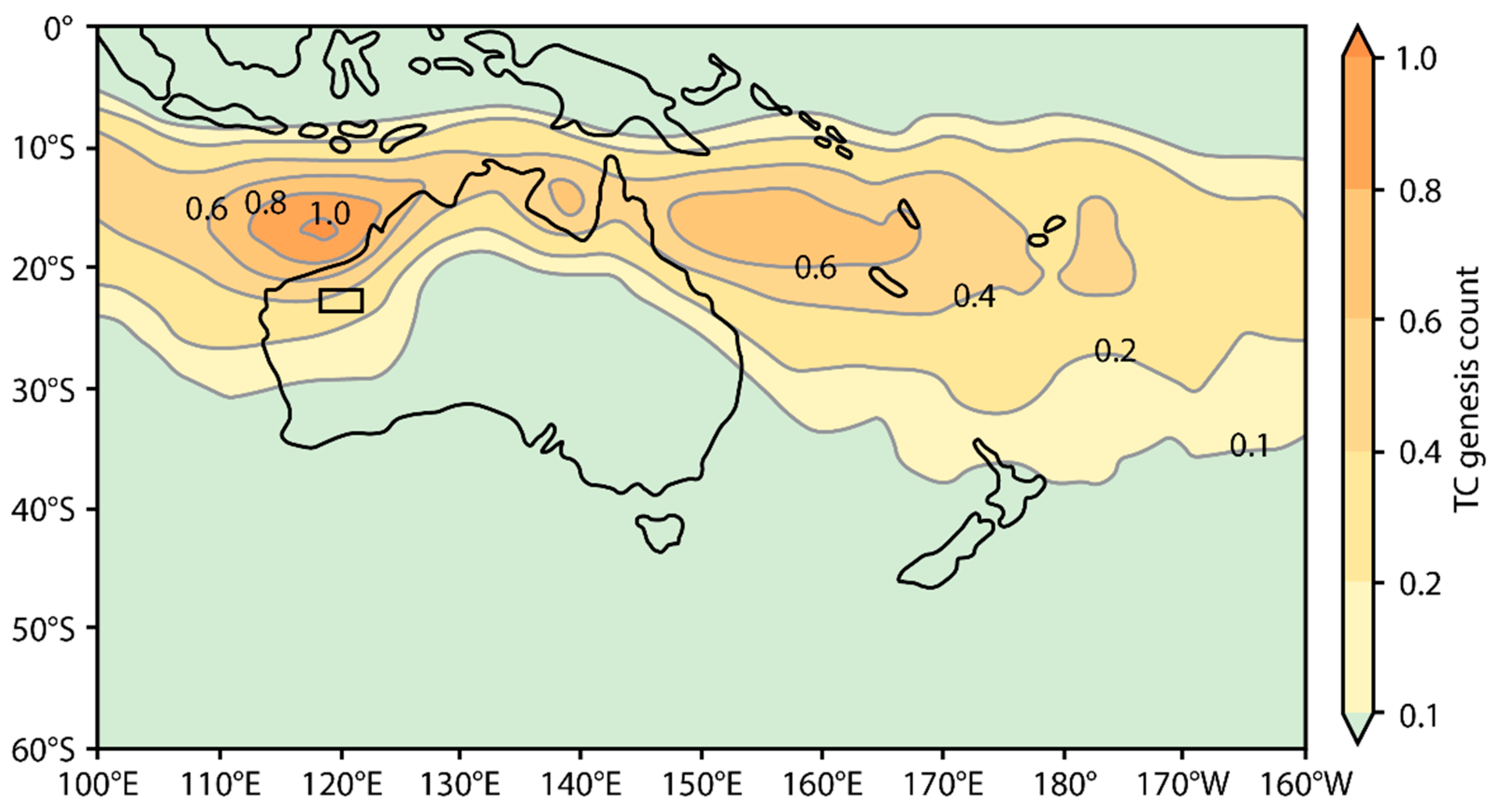
Figure 1. Observed Southern Hemisphere Tropical Cyclone genesis counts (all seasons) indicating the 122 average annual number of tropical cyclones through Australian region in El Niño, La Niña, and neutral 123 years (modified from Australian Government Bureau of Meteorology, 2019 [36]).
Hydrology 09 00165 g001
Figure 2. Workflow of steps to determine Regional Flood Frequency Estimation (RFFE) selection and for small headwater channels.
Hydrology 09 00165 g002
Figure 3. Adopted regions for RFFE technique in Australia. Modified from Rahman et al., (2019) [52]. The Fortescue Catchment, Pilbara is outlined.
Hydrology 09 00165 g003
Figure 4. Map of headwater catchments used to test RFFE methods. Numbered catchments border the Yandi Mine in Eastern Pilbara, WA.
Hydrology 09 00165 g004
Figure 5. Single location IFD design rainfall plot (Catchment 1). Legend shows Annual Exceedance Probability (AEP) expressed as a percentage. Output from BOM Design Rainfall Data System [60].
Hydrology 09 00165 g005
Figure 6. Design rainfall patterns for 5% AEP 12 h storm.
Hydrology 09 00165 g006
Figure 7. Catchment with a digitized white line showing a cross section (Plot output) for the TUFLOW model.
Hydrology 09 00165 g007
Figure 8. Catchments used in sensitivity analysis. (a) Catchment 1—A small shallow unconfined catchment with multiple flow paths, (b) Catchment 5—A steep, confined catchment and (c) Catchment 10—An unconfined single thread channel within a larger catchment. Graphs show the contour data of the longitudinal profile of the river channel. The red dashed line shows the equal area slope.
Hydrology 09 00165 g008
Figure 9. Comparison of small flood predicted peak discharges using RFFE approaches [2,15,17,18] for Q2, Q5, Q10, Q20, Q50 and Q100 return intervals.
Hydrology 09 00165 g009
Figure 10. IFM [18], ARR RFFE and RFFP2000 [17] approaches compared with results from direct rainfall modelling from TUFLOW for the modelled headwater catchments.
Hydrology 09 00165 g010
Figure 11. Sensitivity analysis box plot to show results for Catchments 1, 5 and 10 for a Q20 flood where Manning’s n, hyetograph shape and grid size were adjusted.
Hydrology 09 00165 g011
Figure 12. Effect of grid size variation in the direct rainfall model. Figure (a) shows 10 m grid, (b) 5 m grid and (c) 2 m grid sizing.
Hydrology 09 00165 g012
Table 1. Regional Flood Frequency Estimation methods applied to headwater catchments.
MethodEquation
ARR (Australian Rainfall and Runoff Regional Flood Frequency Estimation Model) RFFE ModelQx = Q10 × GFx
with Q10 as: log10 = b0 + b1 log10 (area) + b2 log10(I6,50) Where b0, b1 and b2 are regression coefficients, estimated using OLS regression, area is the catchment area in km2 and I6,50 is the design rainfall intensity at catchment centroid for a 6 h duration and 50% AEP. The values of b0, b1 and b2 and the regional Growth Factors (GFx) are embedded into the RFFE Model 2015.
Index Flood Method (IFM) (Davies and Yip, 2014) [18]For a small catchment area: Q5 = 7.32 × 10⁻⁸ A0.651 I1hr, 2 yrs5.251
Frequency Factors: 2ARI = 0.31, 5ARI = 1.0
10 ARI = 1.70, 20ARI = 2.58, 50ARI = 4.15, 100ARI = 5.82
Parameter Regression Technique (PRT) (Taylor et al., 2011) [15]M = −11.411 + 0.527 × ln(area) + 7.765 × ln(I12hr,2)
S = C1:g = C2 where C1 and C2 are regional average M = 2.54 + 0.52[ln(area) − 4.71] + 8.08[ln(I12,2) − 1.47]
Fixed Region Parameter Regression Technique (PRT) (Rahman et al., 2012a) [2]M = 2.54 + 0.52[ln(area) − 4.71] + 8.08[ln(I12hr,2) − 1.47]
stdev = 1.45 + 0.10(zarea) + 0.07(zforest) (4.8.17) skew = −0.49 − 0.08(zarea) − 0.64(zsden) (4.8.18)
Quartile Regression Technique QRT (Taylor et al., 2011) [15]ln(Q2) = −11.366 + 0.521 × ln(area) + 7.858 × ln(I12hr,2) ln(Q5) = −15.913 + 0.486 × ln(area) + 5.336 × ln(I1hr,2)
ln(Q10) = −14.285 + 0.465 × ln(area) + 5.055 × ln(I1hr,2) ln(Q20) = −12.949 + 0.445 × ln(area) + 4.824 × ln(I1hr,2) ln(Q50) = −4.914 + 0.431 × ln(area) + 5.705 × ln(I12hr,2) ln(Q100) = −4.072 + 0.413 × ln(area) + 5.412 × ln(I12hr,2)
Quartile Regression Technique QRT (Rahman et al., 2012) [2]ln(Q2) = 2.66 + 0.51(ln(area) − 4.71) + 8.08 [ln(I12,2) − 1.47]
ln(Q5) = 3.90 + 0.48[ln(area) − 4.71] + 7.20 [ln(I12,2) − 1.47]
ln(Q10) = 4.51 + 0.45[ln(area) − 4.71] + 6.74 [ln(I12,2) − 1.47]
ln(Q20) = 5.01 + 0.44[ln(area) − 4.71] + 6.19 [ln(I12,2) − 1.47]
ln(Q50) = 5.59 + 0.41[ln(area) − 4.71] + 5.66 [ln(I12,2) − 1.47]
ln(Q100) = 5.87 + 0.39[ln(area) − 4.71] + 5.34 [ln(I12,1) − 1.47]
RFFP (Flavell, 2012) [17]Q2 = 1.72 × 10−64(ASe0.5)0.8 LAT−12.17 LONG38.77 (L2/A)−1.05
Q5 = 7.47 × 10−46(ASe0.5)0.81 LAT−14.62 LONG31.40 (L2/A)−0.68
Q10 =2.36 × 10⁻³⁴(ASe0.5)0.81 LAT−15.24 LONG26.28 (L2/A)−0.39
With the largest value from two Q20 equations being adopted for the Q20 value:
Q20 = 1.98 × 10 − 23(ASe0.5)0.79 LAT−15.08LONG20.91
Q20 = Q10 = (13.21A0.61)/(8.74A0.60)
Q50 = Q20 × frequency factor (Q50/Q20)
Q100 = Q20 × frequency factor (Q100/Q20)
A = catchment area (km2), Se = equivalent uniform slope (m/km) and L = mainstream length (km)
Table 2. Catchment description for RFFE and direct rainfall analysis.
CatchmentArea (km2)LatitudeLongitudeSe (m/km)L (km)
11.05−22.711924118.95589218.541.13
20.96−22.694436119.00158540.570.71
31.68−22.695323119.04588216.651.10
41.48−22.690506119.08705822.971.64
51.71−22.697491119.08453337.611.55
61.95−22.732084118.96519512.491.37
75.99−22.765762119.15932222.482.06
83.23−22.804315119.16140122.721.30
91.1−22.795682119.10915626.711.17
102.42−22.735894118.98030916.851.21
Table 3. ARR rainfall depths (mm) for a 12 h storm per AEP (%).
CatchmentArea (km2)50AEP20AEP10AEP5AEP2AEP1AEP
11.052.356.7511.016.023.329.0
20.962.376.7811.016.123.429.1
31.683.349.5915.622.733.141.2
41.483.329.5215.526.632.840.9
51.713.5910.316.824.435.544.3
61.953.229.2415.121.931.939.7
75.997.2120.733.749.071.388.9
83.234.7013.522.032.046.558.0
91.12.597.4412.117.625.632.0
102.423.7210.717.425.336.845.9
Table 4. Modelled peak discharges using the direct rainfall modelling approach for a 12 h rainfall event across average return intervals. Peak discharge values are in m3 s−1.
Catchment2ARI5ARI10ARI20ARI50ARI100ARI
10.517.7516.5617.5858.1077.79
32.2410.6312.4519.3930.3783.30
40.802.683.5018.4121.2262.69
52.8810.1127.4032.5670.25120.11
61.385.757.327.506.3258.53
74.169.6052.072.6676.7387.60
80.201.9552.2961.2668.8285.86
92.202.379.7810.9762.24128.20
100.643.7210.717.425.336.80
Table 5. Results of sensitivity analysis catchments 1, 5 and 10 for the 20ARI.
CatchmentGrid SizeHyetographManning’s nQpeak (m3 s−1)
1570.02818.76
1570.03513.71
1570.04211.02
1510.03517.22
1520.0357.38
1530.03514.24
1540.0358.67
1550.03510.70
1560.0356.68
1570.03513.71
1580.0359.98
1590.03513.58
15100.03513.66
1270.03510.54
1570.03513.71
11070.03521.61
5570.02826.62
5570.03513.30
5570.0429.86
5510.0357.87
5520.03510.75
5530.03517.36
5540.03518.90
5550.03513.01
5560.03511.60
5570.03513.30
5580.0357.92
5590.0359.25
55100.0356.29
5170.0358.93
5270.03510.10
5570.03513.30
51070.03546.21
10570.0289.48
10570.03515.45
10570.0427.80
10510.03514.28
10520.03514.66
10530.03516.96
10540.03516.00
10550.03517.55
10560.03520.34
10570.03515.45
10580.03520.22
10590.03515.27
105100.03521.91
10270.03520.82
10570.03515.45
101070.03533.98
Publisher’s Note: MDPI stays neutral with regard to jurisdictional claims in published maps and institutional affiliations.