Abstract
In flood area mapping studies, hydrological-hydraulic modeling has been successfully applied around the world. However, the object of study of most of the research developed in Brazil is medium to large channels that use topographical and hydrometeorological data of coarse spatial and temporal resolution. Thus, the aim of this study is to investigate coupled modeling in a small urban channel, using high-resolution data, in the simulation of flood events in a small urban channel, located in Campo Grande, Mato Grosso do Sul. In this study, we used the HEC-HMS and HEC-RAS programs, where topographic information, land use, land cover, and observed data from rain gauges, water level, and flow sensors from 2015 to 2018 were used as input data. To calibrate and validate the hydrological model, four events were used that occurred during the monitoring period, while in the hydraulic model we chose a historical event that caused great disturbances. We then generated flood scenarios with representative synthetic rainfall for a basin, with return times of 5, 10, 50, and 100 years. We observed a good fit in the calibration and validation of the HEC-HMS, with values of R2 = 0.93, RMSE = 1.29, and NSE = 0.92. In HEC-RAS, we obtained values of R2 = 0.93, RMSE = 1.29, and NSE = 0.92 for the calibration, and in the validation, real images of the event prove the computed flood spot sources. We observed that rain with a return time of less than five years provides areas of flooding in several regions of the channel, and in critical channeled sections, the elevation and speed of the flow reach 5 m and 3 m·s−1, respectively. Our results indicate that the channel already has a natural tendency towards flooding in certain stretches, which become more compromised due to land use and coverage and local conditions. We conclude that the high-resolution coupled modeling generated information that represents local conditions as well, showing how potential failures of drainage in extreme scenarios are possible, thus enabling the planning of adaptations and protection measures against floods.
1. Introduction
There has been growing concern about the risk of flooding in Brazil and worldwide, mainly with issues related to the rapid urbanization of cities [1,2], the occupation of high-risk areas [3], and extreme rainfall events [4]. Thus, it is crucial to map areas that may be affected by floods, so that decision-makers create their workflows, whether for containment, mitigation, or nuisance prevention, ensuring that the population has full conditions to develop their social and economic activities.
The use of coupled hydrological and hydraulic models is considered one of the most widespread methodologies for mapping floods [5]. Applications of these models are varied, including real-time flood forecasting systems [6], economic assessment of consequences [7], engineering works, whether hydraulic or not [8], city planning [9,10], as well as research involving erosion, and sediment transport processes [11].
While hydrological models are usually executed quickly, with several well-defined methodologies for each stage of the water cycle, hydraulic models can be computationally expensive, and the accuracy is dependent on the data resolution used. Hydraulic models can be classified according to the dimensionality of the calculations (1D, 2D, or 3D), with [12] indicating 2D models (based on the complete shallow water equation) as the first choice for general surface runoff simulation. Two-dimensional models offer a good advantage for mapping flood areas as they can simulate the dynamics of lateral flows of a floodplain connected to a channel, as in 1D models [13], and without the need for large computational power and time to simulate large areas, as in 3D models [14].
In these models, there is a myriad of programs that can be used, and the modeler should choose one of them, based on the features offered. In studies carried out in Brazil, there are successful applications of the HEC-HMS/HEC-RAS [15], as well as the SWMM and its commercial derivatives [16]. However, there are difficulties in configuring and validating flood simulations in urban channels, mainly on small scales and in developing countries, due to the high sensitivity of these models to topography [17] and flow/rainfall data series [18], usually found in open regional or global databases.
In Brazil, for example, few locations have high-resolution topographic databases available, therefore, in hydrodynamic models, combinations of local topographic surveys with global digital models are used [19]. The same data resolution problem is found in hydrological databases (rain-gauges and level-gauges) as the main national provider is the Brazilian Water Agency (ANA), which provides data with daily resolution [20,21].
Therefore, the objective of this study is to provide parameters of comparison, so that other researchers can evaluate their own approaches to modeling flood events, in small urban channels. For this, we describe and perform a coupled hydrological-hydraulic modeling, with data at a high level of detail (in terms of Brazil) in a small urban basin, located in the municipality of Campo Grande, Mato Grosso do Sul. To this end, we used the HEC-HMS and HEC-RAS programs, having as input data a digital terrain model (MDT) with fine spatial resolution, and a series of precipitation and stages monitored sub-hourly from 2015 to 2018. In this study, we also investigated the behavior of main basin drainage when exposed to design precipitation events, with return periods (RP) of 5, 10, 50, and 100 years.
2. Materials and Methods
2.1. Study Area
The study was carried out in the Prosa stream basin (Figure 1), located within the urban perimeter of Campo Grande, Mato Grosso do Sul, covering 25 neighborhoods (including the center), with a contribution area of 31.97 km2, and a perimeter of 28.63 km. In addition to Prosa, there are six other macro-drainage channels, the Sóter, Vendas, Reveillón, Desbarrancado, Joaquim Português, and Pindaré streams. These channels run in various configurations, alternating from open sections in a natural bed to closed channels, with bridges and culverts modifying the flow along the way.
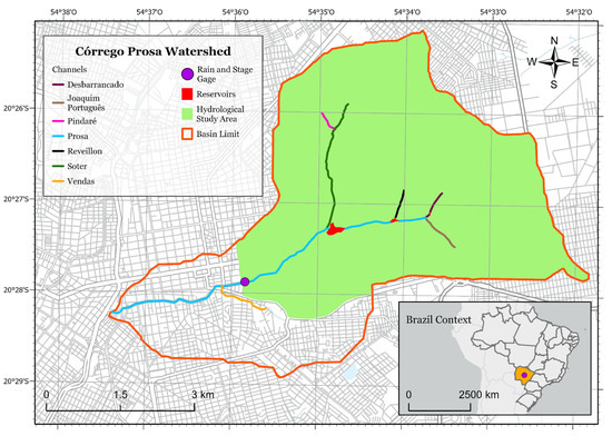
Figure 1.
Location and situation map of the Prosa basin, in Campo Grande, MS, Brazil.
According to data from rain gauge 2,054,014 (managed by ANA, National Water Agency), the average rainfall in the basin in the period from 1976 to 2015 is 1445 ± 273 mm. It should be mentioned that January is the month with the most rainfall (218 ± 84 mm) and August is the driest month (34 ± 34 mm). Therefore, the climate is tropical with a dry season. The rainy season coincides with the summer and the dry season with the winter [22]. Average temperatures range from 25.1 °C in January to 20 °C in July, according to National Meteorology Institute (Instituto Nacional de Meteorologia, INMET).
For the development of the study, we used data from a rain gauge and a level sensor, with sub-hourly data (1 min resolution) available from 2015 to 2018. To use this sensor data as a boundary condition in hydrological studies, we consider the basin outlet at the sensor position. For hydraulic modeling, based on historical spots recorded by local media vehicles, the study area was delimited to 80 m on each side of the axis of the open channels (average length of one urban block), in urbanized areas, and in all the parks.
2.2. Flood Problem in Prosa Basin
For more than a decade, the local press in Campo Grande has been reporting rain events that caused issues related to urban drainage [23,24,25,26,27,28,29]. The Prosa basin is known for its various flooding and inundation points, which have already cost more than 81 million reais to public coffers in containment and remediation works [23]. Regarding the floods, Arq. Avenida Rubens Gil de Camilo (popularly known as Via Parque, Figure 2) and Avenidas Ricardo Brandão and Fernando Correia da Costa concentrate on the largest number of occurrences of this kind of disaster (Figure 2). In these places, not only the elevation of the water depth, but the flow velocity is also responsible for the reported problems.
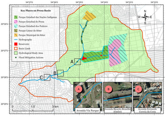
Figure 2.
Key places in Prosa basin.
2.3. Study Workflow
The work was divided into three stages (Figure 3). The first part refers to the calibration and numerical validation of the hydrological modeling, in which the parameters and geometric mesh are derived from the model developed by [30]. Afterward, we have the calibration and numerical/visual validation of the hydraulic model, which obtains representative synthetic rainfall for the study area, with return times of 5, 10, 50, and 100 years, and a generation of risk and exposure maps, for these events.
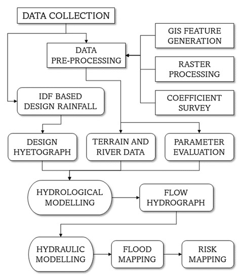
Figure 3.
Workflow to mapping flood areas.
2.4. Study Data
To perform the hydrological-hydraulic modeling, some information is required. For the topography, we used the digital terrain model (DTM) with a spatial resolution of 1 m, developed by a city hall’s aerophotogrammetric survey in 2013. In addition, for the mapping and generation of vector layers, we used two orthophotos: one from 2013 (with 0.1 m spatial resolution) derived from an aerial survey, and another from 2016 (with 0.6 m spatial resolution) derived from satellite imagery [31].
Bathymetric surveys were carried out in four reservoirs, and some channel’s reaches, based on common topographic leveling in areas with shallow water, and with the Acoustic Doppler Current Profiler (ADCP) in sections with a depth greater than 0.5 m and reservoirs.
Campaigns for the survey of sections were also carried out, complementing information on the channel’s geometry, also obtained by the public authorities, and companies specialized in the field of hydraulic engineering, in a total of 52 cross sections.
We also used precipitation and water level data, with both sensors providing data every 1 min, from 2015 to 2018. To establish a rating curve for the outflow section, we performed measurements with ADCP during the recession of an intense precipitation event (35 mm in 1.25 h), measuring the flow continuously while the channel level decreased, ending at the limit of the sensor scanning capacity.
2.5. Design Rainfall
To determine synthetic precipitation events, we used probability distributions applied to Campo Grande’s IDF (Intensity-Duration-Frequency) curve, available in the Urban Drainage Master Plan [31]. This was based on a series of daily precipitation data, obtained by the rain gauge numbered 2,054,014 (see Section 2.1), over a period of 30 years.
where: is the rainfall intensity in mm/h, a function based on the return period, in years; a function, based on rain duration time, in minutes.
To choose a rainfall distribution that best represents the hyetographs of significant rainfall events recorded in the basin, we applied two methodologies, referring to the evaluation of geometric parameters [32] and peak [33], comparing the events captured by the rain gauge (Figure 4) with those determined by the distributions. We consider the ten most intense precipitation events in the data series used to be significant.
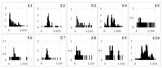
Figure 4.
Hyetographs of heavy rains captured by the Prosa rain gauge. Each “E” event has an associated numerical identifier, with intensity in mm/h on the vertical axis and duration in h on the horizontal axis.
Three parameters were determined to verify the hyetographs, including:
Normalized peak time : position of the time at which the rainfall peak intensity occurred, divided by the total duration of the event.
Normalized centroid : time position of the centroid of the hyetogram, divided by the total duration of the event. The centroid of a hyetogram with temporal resolution , can be calculated by summing the centroids of the rainfall intensity bars, as in Equation (3), where is the rainfall intensity in time step , and is the total rainfall.
Normalized peak difference : an absolute value of the difference between the mean peak of events and the peak of the distribution, divided by the mean peak.
The distributions chosen for the calculation were those that allow a direct connection with the IDF curves, including Rectangular (RET), Sifalda (SIF), Triangular (TRI), Double Triangle (DTR), Linear Exponential (LEX), and Alternated Blocks (BLO). All were calculated with parameters based on the means of significant rainfall events recorded by the rain gauge at the outlet, lasting 1.5 h and with a return time of 0.026 years. The return time of events was obtained by isolating the variable in the IDF curve. Table 1 collects data from the events, as well as the metrics calculated for each one of them and the averages, used as a test parameter for the distributions.

Table 1.
Significant rainfall events observed by the outfall station, and their metrics.
2.6. Hydrological Modelling
The Hydrologic Modeling System (HMS) is a program developed by the United States Army Corps of Engineers (USACE). According to [34], it has the ability to perform the physical description of basins, as well as the meteorological description of events, allowing hydrological simulations and optimizations [35], forecasts of flow and scenario tests [36], uncertainty analyses, and studies involving sediment and/or water quality [37].
The HEC-HMS is a concentrated model with a modular program, in which each step of the hydrological cycle is executed in a chain, and in this study, there are four steps to be modeled. For this purpose, we divided the Prosa basin into 16 sub-basins (Figure 5), aiming to maximize the distribution of surface runoff along the drainage channels.
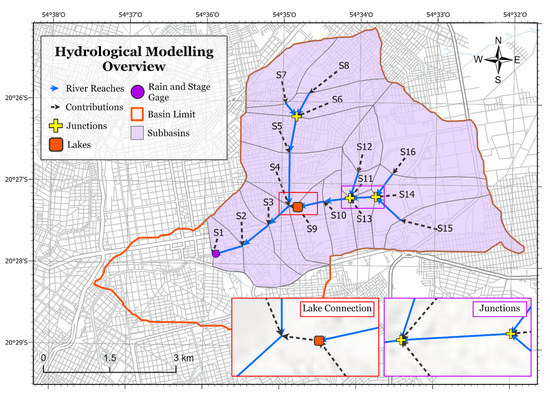
Figure 5.
Mesh elements in the HEC-HMS watershed model configuration.
The losses module was configured using the Curve Number methodology of the National Resources Conservation Service-NRCS (former SCS-CN method), where a CN value was assigned to each basin. In the same way, the methodology chosen for the transformation module was the Clark unit hydrograph, and the concentration time and storage coefficient of the basins were determined using the TR-55 recommendations [38] and the Nash model [39], respectively.
To represent the base flow, the recession method was used, parameterized by the variables threshold flow, and the decay coefficient [40]. Finally, the channel flow module was configured using the semi-conceptual Muskingum-Cunge method, which has the cross-sections of the macrodrainage channels (1D) as a parameter, as well as the roughness of the surface (given by Manning’s n).
For calibration and validation, we varied the CN values, as well as the roughness of the cross sections, using the rain events E2, E3, E8, and E9, as the stage recorded in these events is within the data set measured by the survey of the rating curve. The calibration was performed by comparing the outlet calculated values with the observed, where in the end, a peak difference was observed and automatically adjusted with optimization attempts. In this approach, we use the objective function Percent Error Peak (PEP), targeting the values of CN and Initial Abstraction.
The data adjustment evaluation, both in the calibration and validation, was done numerically, using the metrics: coefficient of determination (R2), Root Mean Square Error (RMSE), and Nash-Sutcliffe efficiency (NSE), automatically calculated by the HEC-HMS:
The R2 represents the degree of correlation of the observed and calculated data, ranging from 0 to 1, and the higher the better. In the equations, c is the value calculated by the model, o is the observed value, and n refers to the data range number.
RMSE represents the average error of predicted data compared to observed data, in which the smaller the better.
NSE corresponds to the comparison of the magnitude of the residual variance calculated with the variance of the observed data set, ranging from −∞ to 1, where NSE > 0 indicates predictive accuracy better than the observed mean. Here, is the average observed value.
Table 2 and Table 3 summarize the coefficients used in the methodologies described above, after the calibration and validation of the hydrological model.
Table 2.
Coefficients used in the operational hydrological model, for hydrological modelling.
Table 3.
Roughness coefficients for the channel sections of the hydrological model.
2.7. Hydraulic Modelling
HEC-RAS (River Analysis System) was used for hydraulic analysis, and similar to the HEC-HMS, is a program developed by the members of the USACE. The shallow water equation, used in analyzes conducted by the software, is a combination of the continuity equation and conservation of momentum. In two-dimensional terms, we can write the complete equations in the following form:
where:
- Equation (8): Continuity equation (conservation of mass). This form is under the assumption of fluid incompressibility. In it, t represents time, u,v the Cartesian components of velocity, x,y the Cartesian directions, h is the height of the water column in the plane fraction studied, and q is the term for the flow source [41].
- Equations (9) and (10): Equations of conservation of linear momentum. This form is under the assumption that the dimensions of the scales of the plane are much larger than the vertical, justifying that the vertical forces cut down to hydrostatic pressure. If the fluid density is constant and without the action of other vertical forces on the fluid, we can neglect the velocity and vertical inertial terms of the Navier-Stokes equation, obtaining the described equations. In these, g is the acceleration of gravity, u,v the Cartesian components of velocity, x,y the Cartesian directions, v_xx and v_yy are the coefficients of turbulent viscosity in the x and y directions, c_f is the term for the coefficient of background friction, τ_s is the wind surface shear stress, h is the water depth, and f is the Coriolis force parameter [41].
The terrain used in the hydraulic modeling is a modification of the original MDT of Campo Grande. Despite having a spatial resolution of only 1 m, the original model does not present in its entirety some elements of drainage and urban occupation (such as canals, gutters, and buildings), which is crucial to generate reliable and accurate flooding patches [42]. Therefore, we generated a new DTM, by creating several layers of altimetry based on existing topographic information (bathymetry, cross sections, and break lines of the urban footprint), and joining them to the base DTM, using a raster mosaic tool, within the GIS environment.
We built the mesh of two-dimensional cells and roughness regions according to the data resolution insights made by [43], to minimize continuity errors during the mapping, either by water leakage to impossible regions, or by the heterogeneity of surface features. The cell grid of this study was generated in an adaptive and quadratic way, in addition to position adjustments using break lines, making the cells parallel to the terrain discontinuities. The roughness layer, for this model, divides the area into 23 land occupation classes, with a spatial resolution of 0.15 m, and whose Manning n was assigned based on tabulated/adjusted values.
Hydraulic structures such as dams, bridges, culverts, and ladders are very common in the Prosa basin and were implemented in the HEC-RAS with a direct approach. In case the program does not have the right tool for this (such as energy dissipation stairs and Prosa waterfall), we proceed by adding equivalent spillways, reducing the size of the computational cells on the edge of centerlines.
The flow data from the HEC-HMS were linked to the hydraulic model as a boundary condition, at the outflow point of each sub-basin. In the general downstream, the hypothesis for the normal depth flow was considered.
Regarding the calculation options, we used a standard shallow water equation, without considering the Coriolis force (due to the small scale), turbulent vortices (require further studies), and drag forces due to winds. To increase the numerical stability of the simulations, the time step was controlled by the program, by the Courant-Friedrichs-Levy condition (Equation (11), where c is the speed of the flood wave, ∆t the time interval of the calculation, and ∆x is the longitudinal length of the cell). Starting from an initial value of 1 s, the Courant number (Cr) ranged from 1 ≤ Cr < 0.45, given the nature of the study [44].
Another measure performed to improve the stability of the simulations (mainly for the initial moments) is the warm-up runs. After these are completed, a restart file is generated, which is then used as an initial condition for the next runs. The calculation parameters are described in Table 4.
Table 4.
Calculation options used for this model and notes on usage.
Flood patch calibration was performed manually for event E4, adjusting Manning’s n values, discharge coefficients, and loss coefficients of the hydraulics structures. These variations were determined according to the element of study, based on the minimum and maximum tabulated values [41] for the situation found in the field.
To verify the degree of adjustment of the calibration, we used the observed level data (outlet monitoring station–Figure 1), and calculated the metrics R2, RMSE, and NSE already discussed. We also calculated the flood patch adjustment measure (F), a parameter used in places with a lack of fluviometric data, which measures how coincident the calculated patch is in relation to an observed patch. In this case, the adjustment ranges from 0 to 100%, with the highest value indicating that the calculated area is equal to the observed area. A_int is the observed (obs) and calculated (cal) area that is flooded (intersection).
The E4 event was chosen because the channel overflowed at several points, on a working day and during the afternoon, which allowed many people and press vehicles to register the event. Thus, we also have videos and images that allow us to validate the extent of the water depth.
3. Results
3.1. Design Rainfall
When applying the rainfall distributions with intensity information to the parameters discussed above, we have the hyetographs represented in (Figure 6). For each of these, we were able to calculate the normalized peak, centroid, and peak time metrics (Equations (2)–(4)), allowing comparison with the mean values of the events recorded in the basin (Table 5).
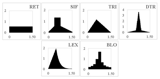
Figure 6.
Hyetographs of rainfall distributions. Intensity in mm/h on the vertical axis and duration in h on the horizontal axis.
Table 5.
Differences between metrics calculated for distributions compared to event averages.
Based on this methodology, it can be observed that the exponential linear model has the best deviation from the hyetograph means in two metrics (−10.94% and −36.35% of centroid difference and normalized peak difference, respectively), and the second-best deviation in relative peak time metric (−30.81%, in which the absolute values were only behind the double triangle model). Thus, the exponential linear model has a geometry that best resembles the significant events recorded in the basin, therefore we will use this distribution to generate synthetic events with an objectified return period (RP, Figure 7).
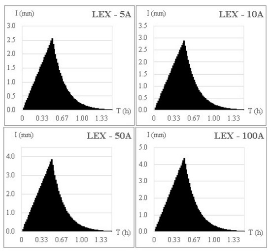
Figure 7.
Hyetographs of synthetic rainfall used in hydrological modeling.
3.2. Rainfall-Runoff Model
The events used for model calibration (Figure 8—E2, E3) presented correlation coefficient (R2) of 0.93 and 0.89, respectively, RMSE of 1.29 m3·s−1 and 0.84, while the Nash-Sutcliffle efficiency coefficient (NSE) varied from 0.92 and 0.89. R2 values close to one attest to the good correlation between the calculated and observed data, while small RMSE values indicate predictive errors of the same proportion. The NSE results close to one suggest the good predictive ability of the application. Among the events selected for validation (E8 and E9), in view of the above reference values, the confirmation of the capabilities of the hydrological model can be observed, with E8 and E9 presenting R2 of 0.96 and 0.9, NSE of 0.94 and 0.89 and RMSE 1.22 and 1.42, respectively.
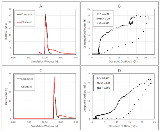
Figure 8.
(A,C): Simulated and observed hydrographs for events E2 and E3, respectively; (B,D) are scatter plots of observed and calculated flow data, E2 and E3 respectively.
Other studies of the same nature, carried out in Brazil, also used some of these metrics to calibrate and validate their hydrological models. [15], applying the HEC-HMS in an urban basin in the city of São Paulo, found NSE ranging from 0.77 to 0.97, and RMSE in the range of 0.47 to 0.19 m3.s−1. While [21], when simulating the hydrology of the Capibaribe River basin in Pernambuco, found NSE from 0.55 to 0.74. [46] can also be cited, in their study in Rio Uma in Pernambuco, where they determined NSE = 0.64 increasing to 0.74 in their events. Based on these values, it can be said that the modeling performed in this work is of comparable quality or even better than those performed in the country, attesting to the predictive capabilities of this application.
As the model presented a good fit in the calibration and validation, we can use it to generate the hydrographs referring to the project rains. For these events, an antecedent condition of median humidity (AMC II) was considered for the CN values. The flow peaks in the outlet section vary from 161.2, 188.1, 271.1, and 317.5 m3·s−1 for return periods of 5, 10, 50, and 100 years, respectively.
According to the rating curve survey, the routing capacity of the outflow section (for a water depth of 5 m) is 135.49 m3·s−1, so that we expect the gutter overflow in all synthetic rains produced, due to the excess flow of 19%, 38.8%, 100.1%, and 134.3% in the events of RP = 5, 10, 50, and 100 years, respectively.
3.3. Hydraulic Modelling
After manual calibration, we compared the observed and calculated data for the E4 event (Figure 9) and found the coefficients of the adjustment metrics R2 = 0.87, RMSE = 0.57 m3·s−1, and NSE = 0.85, attributing acceptable likelihood with reality to the HEC-RAS. In the comparison of hydrographs, a peak difference of 8.4% between the compared values can be observed, and the period of the rise of the flood wave was better simulated than the recession. This behavior may be linked to various effects, such as terrain roughness characteristics, overestimated terrain volume storage (MDT altimetric errors), in addition, to the inability of the HEC-RAS model to deal with the micro drainage network, which accelerates the flow propagation process.
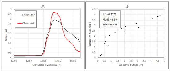
Figure 9.
(A) Comparison of computed and observed hydrographs; (B) Scatter plot for computed and observed stage values (correlation), for event E4, in HEC-RAS.
The standard numerical criteria used to assess the quality of the model (R2, RMSE, and NSE) do not have a basis for comparison in Brazilian studies as there is a lack of fluviometric data that allow modelers to compare calculated and observed data. Using the F graphic criterion to determine the coincidence of the generated spots, our application of HEC-RAS generated a 68% equivalent to the real spot. Considering that this index can reach 100%, the value performed by this model is relatively satisfactory, but there is room for improvement, using a terrain that is closer to reality. Using the same program, refs. [19,21] found values of F 67.5–77% and 66%, respectively, indicating that our application is performing at the level of studies of this type in Brazil.
Based on the information transmitted by the residents and using images made available on social networks and media vehicles, we proceeded with a visual validation for the records of several locations along the basin. This was not only restricted to the extent of the floodway, but we also verified the flow behavior. However, it is important to make it clear that given the model’s limitation in not considering the micro drainage network, water depths generated by storm drains cannot be visualized.
3.3.1. Model Stability
As expected, the presence of many different hydraulic elements (and consequently discontinuities in the resolution methodologies), characteristic of urban areas, led to noise in the simulation results (spikes on hydrographs), mainly in the initial moments. The warm-up period simulation managed to stabilize these initial oscillations (in terms of water depth), from 0.5 m to 0.01 m ranges. The output restart file, used as the initial condition for all other events, improved the overall stability of the simulation.
Another point of concern is the presence of vertical discontinuities in the model since the shallow water equation was not theorized for this type of situation. However, it was found that the adoption of equivalent spillways (calculated by the weir equation), generated smooth hydrographs, without compromising the final response, and could be used.
3.3.2. Flood Mapping: Via Parque Avenue
In the region of Avenida Rubens Gil de Camilo, between the junction of the Prosa and Sóter streams to the exit of the lake, the flood spot computed for the E4 event has an area of 0.032 km2, close to the 0.039 km2 of the observed spot, thus making a percentage difference of 17.95% (Figure 10). The affected area validates journalistic information as the water in the channel is more restricted on the side of the avenue next to the channel, with an overflow section close to the entrance of the closed section that crosses the track.
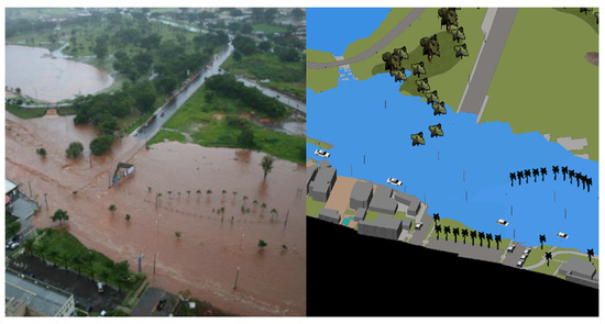
Figure 10.
Comparison of real (left) and computed (right) max floodway extension for the Via Parque region. No scale. Real image reproduced from Campo Grande News.
Analyzing the flood spots (Figure 11), we noticed that during the calibration event there were no buildings affected. As we increase, the TR of synthetic rain, we see an increase in the affected area, with 0.032 km2, 0.040 km2, 0.051 km2, and 0.054 km2 for event E4 and RP = 5, 10, 50, and 100 years, respectively. Moreover, note the progressive number of affected buildings, in the block immediately lateral to the canal. The duration of the flood was slightly impacted by the intensity of the rain, with the presence of water on the side of the stream for 2.00 h in the calibration event, increasing to 2.46 h, 2.50 h, 2.56 h, and 2.58 h in the other simulated scenarios. Considering the worst-case scenario (RP = 100 years), the flooding takes 0.6 h to reach nearby buildings, starting from the time when the synthetic rain started.
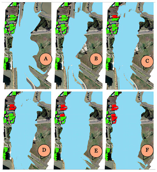
Figure 11.
Flood spots in the Via Parque region. (A) is the observed spot, reconstituted from images of the event. (B) is the simulation for the same event. (C–F) are the simulations of synthetic rain with RP = 5, 10, 50, and 100 years, respectively. Blocks in green and red represent safe and affected buildings, respectively.
In the Via Parque region, in sections close to the channel junction, the HEC-RAS shows a ripple in the longitudinal profile results (such as a hydraulic jump), in all simulations, caused by a step in the channel bed. Although there is no level information in this section to verify the ripple amplitude, social media images on the day of the event reveal the presence of this behavior in the channel, validating the computed result. This phenomenon, however, is not verified when we try to run the model with another set of equations (Diffusion Wave), corroborating the hypothesis that for situations of rapid elevation of the hydrograph (such as these rainfall events in urban areas), and the presence of complex structures, the shallow water equation was the one that was able to capture more details of flow behavior.
3.3.3. Flood Mapping: Ricardo Brandão Avenue
In the region of Av. Ricardo Brandão (near the outflow section), the calibration event caused flooding in the properties facing the Prosa stream, converging with visual information, provided by the news. When analyzing the digital terrain model, we found that the region is naturally prone to flooding as the undulating terrain characteristic of the region becomes locally flat, reducing the height of the constructed channel, mainly on the left bank (in the direction of the flow), where the affected properties are located (Figure 12).
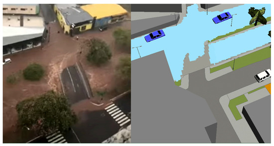
Figure 12.
Comparison of the actual (left) and computed (right) max flood extension, for Av. Ricardo Brandao. Real image reproduced from Youtube and computed by the authors.
The flood spot (Figure 13) for this area has 0.008 km2 for the event of 12/05/2015 (E4—calibration), followed by the synthetic events in 0.010 km2, 0.014 km2, 0.017 km2, and 0.019 km2, for the times of increasing recurrence. From the E4 event to the RP = 100 years, we have an increase of approximately 90% in the flooded area. Regarding the water heights, considering the midpoint of the avenue next to the level sensor, we have a submersion of 0.43 m, 0.70 m, 0.85 m, 1.20 m, and 1.29 m, for the same events. In this parameter, we noticed a significant increase of 200% between events E4 and TR = 100 years.
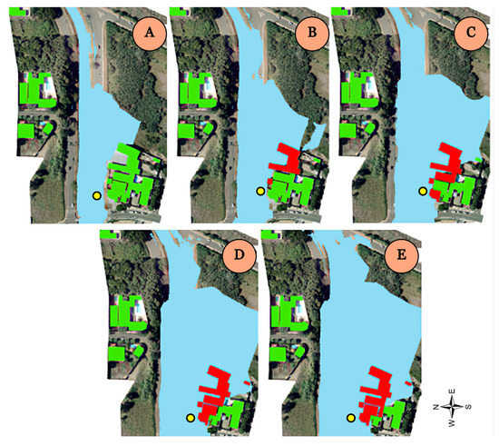
Figure 13.
Flood spots for the Av Ricardo Brandão region. From the letters (A–E), we have the areas related to the calibration event and RP = 5, 10, 50, and 100 years, respectively. Blocks in green and red represent safe and affected buildings, respectively. The yellow point is the location of water level measuring.
The duration of the flooding in this region (the test point being on the avenue, next to the stage sensor) was changed with the intensity of the rain, starting from 0.66 h in the calibration event, rising to 1.06 h, 1.23 h, 1.68 h, and 1.91 h in subsequent modeling. Note that in this region, the time in which the area was submerged was shorter, probably due to the greater capacity of the canalization project (in relation to the section of Via Parque). Considering the largest event computed, the time of arrival of the flood wave in nearby properties was 0.48 h, from the beginning of the rain.
The risk to buildings also increased with the time of recurrence, as a greater number of buildings were affected by water. It is worth mentioning that several buildings in this region have a degree of resilience to floods due to the higher elevation of the foundation (earth slopes) or even with protection walls, but with rains above RP = 10 years, the water level is sufficient to reach these buildings.
3.3.4. Flow Velocity
The authors of [47] discuss the effects of flow velocity on potential damage caused by floods, suggesting that this indicator is the main one to be considered when dealing with damage to pavements. In the Prosa simulation, we see several points with the water velocity in the channel exceeding the standard limit of 3 m·s−1 for protecting plain concrete channels, which validates images of damaged sections after successive flood events. Among the critical stretches for damage caused by high speeds is the exit of the closed gallery of Via Parque (3.35 m·s−1), repeated steps in the downstream sections (6.02 m·s−1), and the exit of dam number 7 (5.39 m·s−1).
While we notice areas of high velocity, we also have stretches where the flow becomes ineffective (flow velocity close to zero), generating ideal recirculation zones for sediment deposition [48], which contribute in the long term to reducing the transport of flow in the channel, increasing the risk of flooding.
4. Conclusions
In this study, we investigated the coupled modeling of a hydrological and hydraulic model (HEC-HMS and HEC-RAS) with topographic and hydrometeorological data of high spatial and temporal resolution in the generation of flood events in a small urban channel located in the municipality of Campo Grande, Mato Grosso do Sul. In addition, we generate flood scenarios with representative synthetic rainfall for the basin, with return periods (RP) of 5, 10, 50, and 100 years.
Our results indicate a good fit in the calibration and validation of the HEC-HMS, with R2, RMSE, and NSE values reaching 0.93, 1.29, and 0.92, respectively, comparable to studies of the same nature carried out in Brazil. In the HEC-RAS, we obtained values of R2 = 0.87, RMSE = 0.57, and NSE = 0.85 for calibration, and its validation, based on graphic criteria, reached F = 68%, the same level as other studies that used this hydraulic model. The median adjustment rate of the flood patch may be linked to deficiencies in the MDT, and therefore the quality of the terrain models used in these studies must be carefully evaluated to increase the accuracy of the patches generated.
Difficulties inherent to two-dimensional hydraulic models, such as initial instabilities and divergence in places with steep slopes and unevenness, can be avoided and minimized, using heating simulations (establishing base flow) and high discretization of the geometric mesh and the time step.
We verified that the Prosa stream is especially vulnerable to floods as rainfall with a low TR of 5 years already provides flooding areas in several regions of the channel. In the outflow section, flows of 130 m3·s−1 lead the channel to an overflow situation, with the water reaching a level 5 m above the bed. Speeds greater than 3 m·s−1 at various points contribute to the deterioration of piped sections, reducing the useful life of hydraulic works.
Our findings show that channels in the Prosa basin have their floodplain compromised due to land use and cover, and local environmental conditions. We conclude that the high-resolution coupled modeling generated information that satisfactorily represents the characteristics of the flow in small channels, portraying the weaknesses of the drainage network in extreme scenarios, and providing authorities with valuable data to carry out efficient planning of use and adjustments that are necessary for vulnerable areas.
Author Contributions
Conceptualization, L.S.B., D.B.B.R. and P.T.S.O.; formal analysis, L.S.B., T.S.M. and P.T.S.O.; funding acquisition, P.T.S.O.; investigation, L.S.B.; methodology, L.S.B., T.S.M. and P.T.S.O.; project administration, D.B.B.R. and P.T.S.O.; supervision, P.T.S.O.; writing—original draft, L.S.B.; writing—review and editing, D.B.B.R., A.A., T.S.M. and P.T.S.O. All authors have read and agreed to the published version of the manuscript.
Funding
This research had support from the Federal University of Mato Grosso do Sul—UFMS/MEC—Brazil, and funded by grants from Conselho Nacional de Desenvolvimento Científico e Tecnológico—CNPq (Grant Numbers: 309752/2020-5, 422947/2018-0) and Coordenação de Aperfeiçoamento de Pessoal de Nível Superior—Brasil—CAPES (Finance Code 001).
Institutional Review Board Statement
Not applicable.
Informed Consent Statement
Not applicable.
Data Availability Statement
Not applicable.
Conflicts of Interest
The authors declare no conflict of interest.
References
- Lin, W.; Sun, Y.; Nijhuis, S.; Wang, Z. Scenario-Based Flood Risk Assessment for Urbanizing Deltas Using Future Land-Use Simulation (FLUS): Guangzhou Metropolitan Area as a Case Study. Sci. Total Environ. 2020, 739, 139899. [Google Scholar] [CrossRef] [PubMed]
- Shao, M.; Zhao, G.; Kao, S.C.; Cuo, L.; Rankin, C.; Gao, H. Quantifying the Effects of Urbanization on Floods in a Changing Environment to Promote Water Security—A Case Study of Two Adjacent Basins in Texas. J. Hydrol. 2020, 589, 125154. [Google Scholar] [CrossRef]
- Pérez-Morales, A.; Gil-Guirado, S.; Olcina-Cantos, J. Housing Bubbles and the Increase of Flood Exposure. Failures in Flood Risk Management on the Spanish South-Eastern Coast (1975–2013). J. Flood Risk Manag. 2018, 11, S302–S313. [Google Scholar] [CrossRef]
- Zhou, Q.; Mikkelsen, P.S.; Halsnæs, K.; Arnbjerg-Nielsen, K. Framework for Economic Pluvial Flood Risk Assessment Considering Climate Change Effects and Adaptation Benefits. J. Hydrol. 2012, 414–415, 539–549. [Google Scholar] [CrossRef]
- Teng, J.; Jakeman, A.J.; Vaze, J.; Croke, B.F.W.; Dutta, D.; Kim, S. Flood Inundation Modelling: A Review of Methods, Recent Advances and Uncertainty Analysis. Environ. Model. Softw. 2017, 90, 201–216. [Google Scholar] [CrossRef]
- Mourato, S.; Fernandez, P.; Marques, F.; Rocha, A.; Pereira, L. An Interactive Web-GIS Fluvial Flood Forecast and Alert System in Operation in Portugal. Int. J. Disaster Risk Reduct. 2021, 58, 102201. [Google Scholar] [CrossRef]
- Pathak, S.; Liu, M.; Jato-Espino, D.; Zevenbergen, C. Social, Economic and Environmental Assessment of Urban Sub-Catchment Flood Risks Using a Multi-Criteria Approach: A Case Study in Mumbai City, India. J. Hydrol. 2020, 591, 125216. [Google Scholar] [CrossRef]
- Elmoustafa, A.M.; Saad, N.Y.; Fattouh, E.M. Defining the Degree of Flood Hazard Using a Hydrodynamic Approach, a Case Study: Wind Turbines Field at West of Suez Gulf. Ain Shams Eng. J. 2020, 11, 741–749. [Google Scholar] [CrossRef]
- Zope, P.E.; Eldho, T.I.; Jothiprakash, V. Impacts of Land Use–Land Cover Change and Urbanization on Flooding: A Case Study of Oshiwara River Basin in Mumbai, India. Catena 2016, 145, 142–154. [Google Scholar] [CrossRef]
- Nithila Devi, N.; Sridharan, B.; Kuiry, S.N. Impact of Urban Sprawl on Future Flooding in Chennai City, India. J. Hydrol. 2019, 574, 486–496. [Google Scholar] [CrossRef]
- Rosas, M.A.; Vanacker, V.; Viveen, W.; Gutierrez, R.R.; Huggel, C. The Potential Impact of Climate Variability on Siltation of Andean Reservoirs. J. Hydrol. 2020, 581, 124396. [Google Scholar] [CrossRef]
- Guo, K.; Guan, M.; Yu, D. Urban Surface Water Flood Modelling-a Comprehensive Review of Current Models and Future Challenges. Hydrol. Earth Syst. Sci. 2021, 25, 2843–2860. [Google Scholar] [CrossRef]
- Merwade, V.; Olivera, F.; Arabi, M.; Edleman, S. Uncertainty in Flood Inundation Mapping: Current Issues and Future Directions. J. Hydrol. Eng. 2008, 13, 608–620. [Google Scholar] [CrossRef]
- Zhang, B.; Wu, B.; Ren, S.; Zhang, R.; Zhang, W.; Ren, J.; Chen, Y. Large-Scale 3D Numerical Modelling of Flood Propagation and Sediment Transport and Operational Strategy in the Three Gorges Reservoir, China. J. Hydro-Environ. Res. 2021, 36, 33–49. [Google Scholar] [CrossRef]
- Gomes Calixto, K.; Wendland, E.C.; Melo, D.d.C.D. Hydrologic Performance Assessment of Regulated and Alternative Strategies for Flood Mitigation: A Case Study in São Paulo, Brazil. Urban Water J. 2020, 17, 481–489. [Google Scholar] [CrossRef]
- dos Santos, M.F.N.; Barbassa, A.P.; Vasconcelos, A.F. Low Impact Development Strategies for a Low-Income Settlement: Balancing Flood Protection and Life Cycle Costs in Brazil. Sustain. Cities Soc. 2021, 65, 102650. [Google Scholar] [CrossRef]
- Zambrano, F.C.; Kobiyama, M.; Pereira, M.A.F.; Michel, G.P.; Fan, F.M. Influence of Different Sources of Topographic Data on Flood Mapping: Urban Area São Vendelino Municipality, Southern Brazil. RBRH 2020, 25. [Google Scholar] [CrossRef]
- Rangari, V.A.; Umamahesh, N.V.; Patel, A.K. Flood-Hazard Risk Classification and Mapping for Urban Catchment under Different Climate Change Scenarios: A Case Study of Hyderabad City. Urban Clim. 2021, 36, 100793. [Google Scholar] [CrossRef]
- Vasconcellos, S.M.; Kobiyama, M.; Dagostin, F.S.; Corseuil, C.W.; Castiglio, V.S. Flood Hazard Mapping in Alluvial Fans with Computational Modeling. Water Resour. Manag. 2021, 35, 1463–1478. [Google Scholar] [CrossRef]
- Speckhann, G.A.; Borges Chaffe, P.L.; Fabris Goerl, R.; de Abreu, J.J.; Altamirano Flores, J.A. Flood Hazard Mapping in Southern Brazil: A Combination of Flow Frequency Analysis and the HAND Model. Hydrol. Sci. J. 2018, 63, 87–100. [Google Scholar] [CrossRef]
- de Arruda Gomes, M.M.; de Melo Verçosa, L.F.; Cirilo, J.A. Hydrologic Models Coupled with 2D Hydrodynamic Model for High-Resolution Urban Flood Simulation. Nat. Hazards 2021, 108, 3121–3157. [Google Scholar] [CrossRef]
- Peel, M.C.; Finlayson, B.L.; McMahon, T.A. Updated World Map of the Köppen-Geiger Climate Classification. Hydrol. Earth Syst. Sci. 2007, 11, 1633–1644. [Google Scholar] [CrossRef]
- Gaigher, C. Com Histórico de Inundações, Campo Grande Registra Problemas Nas Mesmas Regiões Há 10 Anos; G1: Campo Grande, MS, Brazil, 2019. [Google Scholar]
- Oliveira, V. Chuva Forte Alaga Casas No Dalva de Oliveira e Assusta Moradores; Veja Vídeo; Campo Grande News: Campo Grande, MS, Brazil, 2012. [Google Scholar]
- Rodrigues, N.; Vasconcelos, N. Córrego Transborda e Carro Quase é Levado Pela Água Na Ricardo Brandão; Campo Grande News: Campo Grande, MS, Brazil, 2013. [Google Scholar]
- Dias, A.M.; dos Santos, A.; Prado, F. Córrego Prosa Transborda, Alaga Avenidas e Bloqueia Trânsito Da Capital; Campo Grande News: Campo Grande, MS, Brazil, 2014. [Google Scholar]
- Maciulevicius, P. Córrego Prosa Alaga Pontos e Assusta Na Avenida Ricardo Brandão; Campo Grande News: Campo Grande, MS, Brazil, 2015. [Google Scholar]
- Oliveira, V. Chuva Na Madrugada Enche Córregos, Alaga Casas e Causa Destruição; Campo Grande News: Campo Grande, MS, Brazil, 2016. [Google Scholar]
- Frias, S. Temporal Provocou Alagamentos Em Toda a Extensão Do Córrego Prosa; Campo Grande News: Campo Grande, MS, Brazil, 2019. [Google Scholar]
- Mattos, T.S. Improving Urban Flood Resilience; Federal University of Mato Grosso do Sul: Campo Grande, MS, Brazil, 2021. [Google Scholar]
- PMCG–Prefeitura Municipal de Campo Grande. Plano Diretor de Drenagem Urbana–Consolidado; DIOGRANDE—Diário oficial de Campo Grande: Campo Grande, MS, Brazil, 2015. [Google Scholar]
- Balbastre-Soldevila, R.; García-Bartual, R.; Andrés-Doménech, I. A Comparison of Design Storms for Urban Drainage System Applications. Water 2019, 11, 757. [Google Scholar] [CrossRef]
- Na, W.; Yoo, C. Evaluation of Rainfall Temporal Distribution Models with Annual Maximum Rainfall Events in Seoul, Korea. Water 2018, 10, 1468. [Google Scholar] [CrossRef]
- Scharffenberg, W. Hydrologic Modeling System HEC-HMS User’s Manual; USACE—United States Corps of Engineers: Davis, CA, USA, 2016; p. 612.
- Azam, M.; Kim, H.S.; Maeng, S.J. Development of Flood Alert Application in Mushim Stream Watershed Korea. Int. J. Disaster Risk Reduct. 2017, 21, 11–26. [Google Scholar] [CrossRef]
- Bhadoriya, U.P.S.; Mishra, A.; Singh, R.; Chatterjee, C. Implications of Climate Change on Water Storage and Filling Time of a Multipurpose Reservoir in India. J. Hydrol. 2020, 590, 125542. [Google Scholar] [CrossRef]
- Kaffas, K.; Hrissanthou, V.; Sevastas, S. Modeling Hydromorphological Processes in a Mountainous Basin Using a Composite Mathematical Model and ArcSWAT. Catena 2018, 162, 108–129. [Google Scholar] [CrossRef]
- USDA–United States Department of Agriculture. Urban Hydrology for Small Watersheds. In Technical Report 55; NRCS—Natural Resources Conservation Service: Washington, DC, USA, 1986. [Google Scholar]
- Spence, C. On the Relation between Dynamic Storage and Runoff: A Discussion on Thresholds, Efficiency, and Function. Water Resour. Res. 2007, 43, W12416. [Google Scholar] [CrossRef]
- Feldman, A.D. Hydrologic Modeling System HEC-HMS: Technical Reference Manual; USACE—United States Corps of Engineers: Davis, CA, USA, 2000; p. 157.
- Brunner, G.W. HEC RAS: River Analysis System—Hydraulic Reference Manual; USACE—United States Corps of Engineers: Davis, CA, USA, 2020; p. 520.
- Arrighi, C.; Campo, L. Effects of Digital Terrain Model Uncertainties on High-Resolution Urban Flood Damage Assessment. J. Flood Risk Manag. 2019, 12, e12530. [Google Scholar] [CrossRef]
- Yalcin, E. Assessing the Impact of Topography and Land Cover Data Resolutions on Two-Dimensional HEC-RAS Hydrodynamic Model Simulations for Urban Flood Hazard Analysis. Nat. Hazards 2020, 101, 995–1017. [Google Scholar] [CrossRef]
- Brunner, G.W. HEC-RAS River Analysis System User’s Manual; USACE—United States Corps of Engineers: Davis, CA, USA, 2016; p. 962.
- Pappenberger, F.; Beven, K.; Horritt, M.; Blazkova, S. Uncertainty in the Calibration of Effective Roughness Parameters in HEC-RAS Using Inundation and Downstream Level Observations. J. Hydrol. 2005, 302, 46–69. [Google Scholar] [CrossRef]
- Neto, O.C.L.; Neto, A.R.; Alves, F.H.B.; Cirilo, J.A. Sub-Daily Hydrological-Hydrodynamic Simulation in Flash Flood Basins: Una River (Pernambuco/Brazil). Rev. Ambient. Água 2020, 15, 1–13. [Google Scholar] [CrossRef]
- Kreibich, H.; Piroth, K.; Seifert, I.; Maiwald, H.; Kunert, U.; Schwarz, J.; Merz, B.; Thieken, A.H. Is Flow Velocity a Significant Parameter in Flood Damage Modelling? Nat. Hazards Earth Syst. Sci. 2009, 9, 1679–1692. [Google Scholar] [CrossRef]
- Lakzian, E.; Saghi, H.; Kooshki, O. Numerical Simulation of Sediment Deposition and Trapping Efficiency Estimation in Settling Basins, Considering Secondary Flows. Int. J. Sediment Res. 2020, 35, 347–354. [Google Scholar] [CrossRef]


Publisher’s Note: MDPI stays neutral with regard to jurisdictional claims in published maps and institutional affiliations. |
© 2022 by the authors. Licensee MDPI, Basel, Switzerland. This article is an open access article distributed under the terms and conditions of the Creative Commons Attribution (CC BY) license (https://creativecommons.org/licenses/by/4.0/).