Synoptic Time Scale Variability in Precipitation and Streamflows for River Basins over Northern South America

Abstract

The synoptic mode of variability (SMV) refers to changes in atmospheric conditions over periods ranging from 2 to 10 days. In tropical regions, this variability is driven by tropical waves that have a clear signal on the wavenumber–frequency power spectra of precipitation. This study uses the ensemble empirical mode decomposition (EEMD) method to identify the SMV in daily precipitation and streamflows in 47 river basins over northern South America. We found the presence of the frequency bands with periods of 3–12 days and 6–18 days, which agrees with the SMV associated with tropical waves that modulate precipitation over the region. Furthermore, our results reveal that variance explained by the SMV in rainfall over each catchment is greater than the variance explained by those SMV in streamflows, which suggests that catchments efficiently filter out this variability. We found that SMV explains from 5% to 20% of streamflow variability for catchments ranging from 1000 km${}^2$ to 5000 km${}^2$. Additionally, the variance explained by SMV decreases as a power fit with the catchment area. Thus, this study characterizes the SMV for potential applications on regional hydrology, diagnosis, modeling, short-time forecasting, prediction, and management of water resources.

1. Introduction

The synoptic mode of variability (SMV) refers to changes in atmospheric conditions over periods ranging from 2 to 10 days [1,2]. SMV is determined by a combination of remote atmospheric teleconnections, sub-seasonal patterns such as atmospheric waves, regional circulations, and local responses of the weather to the synoptic state perturbations [3,4]. Furthermore, this high-frequency mode is crucial for short-term weather forecasts and other purposes [5]. Particularly, in the tropical regions, synoptic-scale variability is mostly associated with perturbations moving parallel to the equator like the Kelvin waves, westward inertio-gravity waves, mixed Rossby-gravity waves (MRG), and easterly waves (EWs) (e.g., [6,7,8]). These waves modulate mesoscale convective systems (MCSs) or individual cloud clusters [8] that control the precipitation at synoptic time scales during the year, particularly in northern South America (NSA) [9,10,11,12,13].

For the hydrological cycle, precipitation plays a key role as the input process, which along with processes, such as latent heat fluxes, soil permeability, land-cover, surface, underground fluxes, among others, determine the streamflows and total evaporation in catchments [14,15]. In this sense, synoptic time scale variability in hydrology has been associated with extreme events of precipitation [16], flooding [17], and landslides [18]. This time scale variability is important for short-time forecast, warnings, and operation and control of projects using water resources that require real-time data as well as for planning purposes that require mainly non-real-time data [19]. However, the literature lacks works about the synoptic time scale variability on historical hydrological data (e.g., precipitation and streamflows) with a daily temporal resolution, which also could provide valuable information at this time scales for improving diagnosis, water balances, simulation of daily time series, prediction, and daily extreme statistics of hydrological variables [19].

To study the SMV in time series, it is necessary to decompose data to detect the main modes of variability, including the synoptic. This procedure is commonly carried out using the Lanczos band-pass filter [20], although, methods, such as empirical mode decomposition (EMD) and ensemble empirical mode decomposition (EEMD) were also shown to be useful at efficiently filtering out hydro-climatic time series, e.g., Salas et al. [21] used EMD to identify the modes of variability in precipitation associated with tropical easterly waves during the El Niño–Southern Oscillation, Carmona and Poveda [22] quantified long-term trends and climate change signals in hydrological variables in Colombia, Wang et al. [23] used the EEMD to improve forecasting using autoregressive models and for runoff time series, and Wang et al. [24] used EEMD to investigate teleconnections with monthly streamflows. They assert that this filtering method can efficiently decompose the physical information contained in the streamflows series in its different periodic oscillations. Then, in this work, we use the EEMD method because (a) this method allows decomposing of the time series in modes of oscillation that are coherent with the physical modes reported in the literature [25,26]; (b) EEMD has been used for several applications in hydrology and earth sciences [21,22,23,24]; and (c) it has been used in the atmospheric context to characterize processes at synoptic time scales, such as African EWs [27].

This study addresses the following aspects related to the SMV of catchments in NSA: (1) characterizing the frequency bands associated with the SMV in the time series of daily precipitation and streamflows using the EEMD method; (2) quantifying the percentage of variance explained by the SMV; (3) characterizing seasonal variance properties of the SMV, and; (4) identifying empirical relationships between variances explained by SMV and the catchment areas. This study is the first work in the region that uses the EEMD non-linear decomposition method to characterize the SMV in daily streamflows for several catchments over northern South America. Furthermore, this research unveils the importance of the SMV for streamflow variability and the scaling relationships between the SMV in streamflows and their corresponding catchment areas.

This work is organized as follows. Section 2 presents materials and methods; Section 2.1 to Section 2.3 describe the region of the study and the datasets. Then, we present the decomposition methods, the spectral analysis procedures, seasonal synoptic anomalies, and the empirical relationships. The results and discussions are presented in Section 3. Finally, the conclusions and future work are included in Section 4 and Section 5, respectively.

2. Materials and Methods

2.1. Study Region and Datasets

We carried out our analysis for 47 river basins with areas ranging from ~1000 to ~900,000 km${}^2$, located over NSA, between ${10}^{\circ }$ S–${18}^{\circ }$ N and ${84}^{\circ }$ W–${50}^{\circ }$ W. The river basins were selected following two criteria: (1) availability of daily streamflow data with more than a 10-year record length, and; (2) less than 15% missing data in streamflow time series. Streamflow gauges and the study region are shown in Figure 1.

The NSA is a very complex region with orographic features that ranges from the high Andes mountain range to the plains of the Orinoco and Amazon River basins [28,29]. Therefore, this region presents great heterogeneity in atmospheric and hydrologic processes at several spatial and temporal scales [30,31,32]. For example, daily precipitation ranges from 0.0 to 30 mm/day (Figure 1), daily mean temperatures ranges from 12 to 24 ${}^{\circ }$C/day [33], and mean evapotranspiration ranges from 2.5 to 5.0 mm/day [34]. Moreover, the available streamflow data indicate daily values that range from 1.5 to 178,846 m${}^3$/s.

2.2. Precipitation

We used precipitation data from the ERA5 atmospheric reanalysis [35], which provided an estimate of a large number of atmospheric, land, and oceanic climate variables around the Earth on a 30 km grid with 137 levels from the surface up to a height of 80 km. Moreover, we used data from the Climate Hazards Group InfraRed Precipitation with Station (CHIRPS) [36]. In particular, we used a spatial domain over NSA at a daily resolution for the period 1981–2019, which is the common period for both datasets.

2.3. Streamflows

We used daily streamflow time series from the Colombian Institute for Environmental Studies (IDEAM or Instituto de Hidrología, Meteorología y Estudios Ambientales), the project SO–HYBAM, and the Global Runoff Data Centre (GRDC) [37].

Table 1. Data description.

Dataset	Number of Series	Period	Available
IDEAM	30	2000–2010	http://dhime.ideam.gov.co
SO–HYBAM	6	2003–2013	https://hybam.obs-mip.fr
GRDC	11	1978–1988	https://www.bafg.de/GRDC

shows the details on the datasets, record length, and the number of streamflow gauges used. Table S1 in the Supplementary Material shows the list of streamflow gauges from IDEAM, SO-HYBAM, and GRDC.

2.4. Data Selection and Processing

We explored the available daily streamflow data in the study region, selecting stations with more than 10 years of continuous records and less than 15% missing data. The missing data were filled with the 10-year mean of the available daily data. That is, if a $X_{i,j}$ was a missing data point for the day i in the year j, we filled it with $\langle X_{i,j}\rangle$, where $\langle ·\rangle$ denotes the daily average over the 10-year length record of data for each streamflow gauge.

2.5. Wave Number-Frequency Power Spectra and Fourier Filters

To get an appreciation of the main tropical atmospheric phenomena responsible for the variability of precipitation in the study region and the periods associated with these phenomena, we calculate a regional frequency-–wavenumber power spectra of ERA5 precipitation, following the method developed by Wheeler and Kiladis [6], with the regional tapering approach from Dias et al. [8]. Such analysis gives information on the tropical waves phenomena responsible for precipitation variability in the region of interest. The regional spectra were centered in NSA, on the longitudinal sector between 160${}^{\circ }$ W and 20${}^{\circ }$ E. To allow a smooth synoptic signal distribution while excluding much of the intraseasonal signal, we used 64-day window segments, overlapping by 13 days, and tapered the data using a Hann window, similar to [38]. Once the main waves responsible for synoptic variability in our study region were identified, we filtered ERA5 precipitation, retaining only the variability associated with each wave. This filtering was performed using inverse Fourier transforms, retaining only the variability on frequency–-wavenumber boxes associated with each wave, using the method proposed by Wheeler and Kiladis [6] and boxes similar to Kiladis et al. [7]. The filtered series were used to geographically locate the variance distribution and its annual cycle associated with each wave in the study region.

2.6. Seasonal Synoptic Anomalies

We used a 5-day mean as a representative temporal resolution for the synoptic time scale for precipitation and streamflows [39]. Then, positive (negative) synoptic anomalies indicated that seasonal means were lower (higher) than the 5-day seasonal averages. For streamflows, particularly, synoptic anomalies were computed as percentages of the long-term mean streamflows. This procedure was done to facilitate the spatial visualization of these anomalies.

2.7. Decomposition of Time Series

The empirical mode decomposition (EMD) method has become a common and a powerful tool in geophysical time series analysis [23,26,40,41]. EMD is useful in decomposing non-linear and non-stationary time series into a set of intrinsic mode functions (IMFs), which are extracted through iterative, adaptive, and temporally local procedures that do not force the data $x\left(t\right)$ to prescribed waves as other traditional decomposition methods (i.e., sinusoidal waves or wavelets) [42]. However, the EMD method has a shortcoming: it is not easy to associate physical variability modes to the IMFs because each IMF contains information in different frequency bands [26,43]. To overcome this mode mixing problem, Wu and Huang [44] proposed the EEMD to decompose the original time series data, $x\left(t\right)$, into a set of IMFs exhibiting scale-consistent oscillation features. Details on the EMD and EEMD methods are presented in the Supplementary Material.

2.8. Synoptic Modes of Variability and Their Variances Explained

After finding the main modes of variability (IMFs) through the EEMD method applied to the daily time series, we used the fast Fourier transform [45] to analyze the spectral composition of each IMF to determine which one exhibited periodicity in the 2–10 day timescale.

For precipitation, we computed a daily time series corresponding to the average over each catchment area, defined by each streamflow gauge station. Then, we decomposed that time series in their IMFs, and computed the Fourier spectrum for each IMF to characterize its spectral composition. For streamflows, we decomposed each single time series for the river basins. Then, we quantified the variance explained by the SMV in the daily time series of precipitation and streamflows using the discrete Fourier transform [45,46]. Parseval’s theorem was used to explain the relationship between the variance explained by the SMV to the total variance of the original signal. Hereafter, we quantified the percentage of variance explained by each SMV as

$$PV(\%)=100\ast \frac{{\sum }_{k=0}^{N-1}{\left|{\widehat{x}}_k\right|}^2}{{\sum }_{k=0}^{N-1}{\left|x_k\right|}^2}’$$

(1)

where ${\sum }_{k=0}^{N-1}{\left|{\widehat{x}}_k\right|}^2$ is the variance explained by each SMV and ${\sum }_{k=0}^{N-1}{\left|x_k\right|}^2$ is the total variance of the original time series (without EEMD decomposition).

2.9. Seasonal Variance Explained by the Synoptic Modes of Variability

We used the r-th sample moment [47] as a quantifier of the variance explained by the SMV during seasons (DJF, MAM, JJA, and SON) as

$$M_r=\frac{1}{N}\sum _{i=1}^N{x}_i^r’$$

(2)

where $x_i$ denotes a time series with the length N. In particular, we used the second moment ($r=2$) that gave us information about the variance. Hence, the seasonal percentage of variance ($PV$) explained is defined as

$$PV(\%)=100\ast \frac{{\widehat{M}}_2}{M_2}’$$

(3)

where ${\widehat{M}}_2$ is the second moment of the SMV, and $M_2$ is the second moment of the original time series. In this way, $PV$ serves to show the geographical locations where the variance of the SMV constitute a percentage of variance of the original time series (without filtering) over NSA.

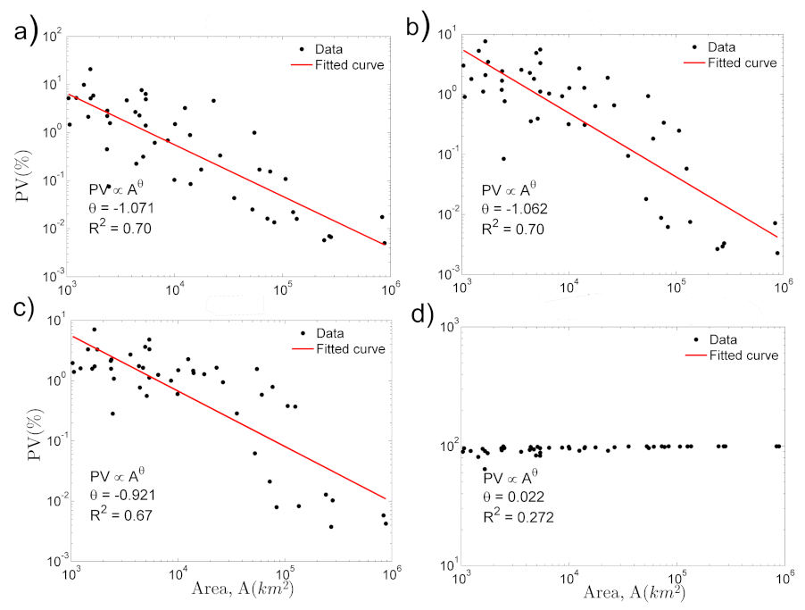
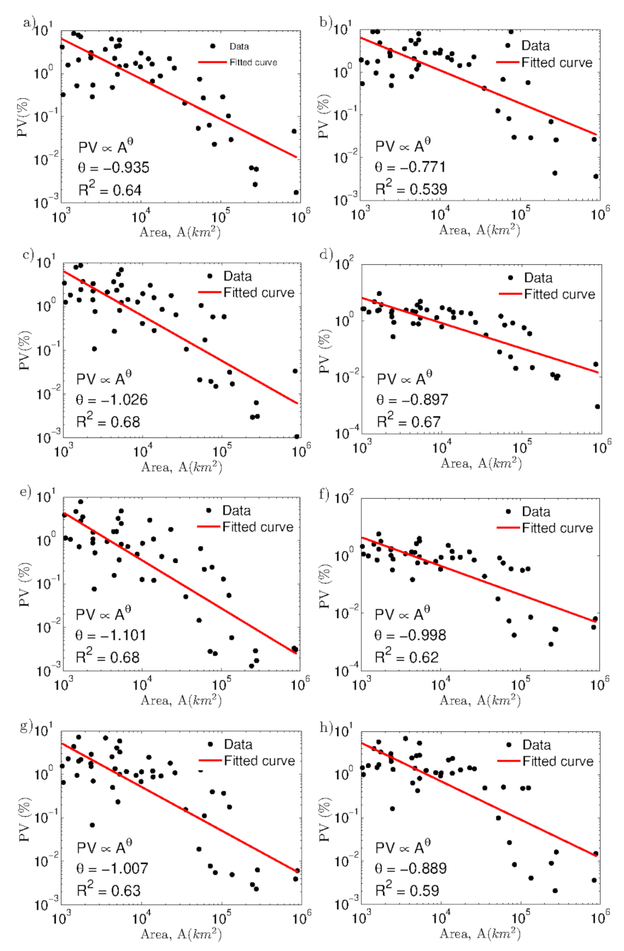
2.10. Relationships between the Variance Explained by the Synoptic Modes of Variability and the Area of Catchments

Hydrology proposes the existence of several relationships between the catchment areas and some of the geomorphological features of the river basins and streamflows [48]. Those relationships look for linkages among attributes, such as discharge, river width, slope, catchment area, and others [48,49]; natural features of catchments and anthropogenic factors that influence the scaling of discharge with drainage area [50,51]; and regionalization of floods [52].

Here, we investigate relationships between the variance explained by the SMV and the catchment areas. To that end, we used a power-fit as

$$PV=c{A}^{\theta }’$$

(4)

where $PV$ is the percentage of variance explained by each SMV, A is the area of the catchment, c is the intercept, and $\theta$ is an exponent. An analogous procedure was done to inquire about relationships between the catchment area and the seasonal percentage of variance, the latter quantified as explained in Equation (3).

3. Results and Analysis

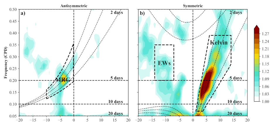
3.1. Wave Number-Frequency Power Spectra and Fourier Filters

The regional spectra of the symmetric and antisymmetric components of ERA5 precipitation for a region centered in NSA are shown in Figure 2. This figure shows the ratio between raw power and the power of a smoothed red noise background spectrum (see [6] for details). Contours beginning at 1.1 indicate that the precipitation variability, due to synoptic-scale phenomena in the NSA region, is driven mainly by Kelvin waves, mixed Rossby-gravity (MRG) waves, and easterly waves (EWs), with a period ranging from 2 to 15 days, representing spectral regions with power more than 10% above the background [53]. Boxes in Figure 2 define wave number–frequency regions corresponding to Kelvin waves, MRG, and EWs, similar to Kiladis et al. [7].

We filtered the ERA5 precipitation using these boxes, retaining only the associated variability with each wave. Figure 3 compares the geographical distribution of the precipitation variance associated with Kelvin waves, MRG, and EWs for the winter (DJF) and summer (JJA) seasons. Figure S1 in the Supplementary Material shows the complete annual cycle for each wave. Figure 3 indicates that the maximum variance tends to follow the latitude of the climatological ITCZ, agreeing with previous works (e.g., [55]), with a clear annual cycle with more variance associated with these waves in the Northern Hemisphere summer. Therefore, the variance associated with synoptic phenomena is geographically concentrated in the NSA, dominated, in order of importance, by the Kelvin waves (Figure 3a,b), followed by the EWs (Figure 3c,d) and the MRG waves (Figure 3e,f). This result agrees with previous works that recognize Kelvin waves as the dominant mode of eastward-moving synoptic-scale disturbances over tropical South America (e.g., [6,56,57,58,59]) and the EWs as important transporters of humidity to NSA [10]. Moreover, it is worth mentioning that our study region is located precisely in the geographical area of maximum variance associated with these synoptic phenomena, which will be relevant for the EEMD analysis that follows.

3.2. Synoptic Modes of Variability in Precipitation and Streamflows

EEMD resulted in three IMFs associated with synoptic variability for precipitation and streamflows. Figure 4 (top row) shows that the precipitation IMF1 exhibit periodicities below 4 days, while the IMF2 contains frequencies associated with periods between 3 and 12 days, and the IMF3 shows periods ranging from 6 to 18 days, which agrees with the periods associated with Kelvin waves, MRG, and EWs. Figure 4 (bottom row) evidences the agreement between the bands of synoptic variability in streamflows and those found for precipitation, mainly associated with IMFs 2 and 3. We point out that all of the time series of streamflow and precipitation analyzed in this work (47 basins) contain frequency bands of synoptic variability. Additionally, Figure 4 indicates that streamflow periodograms are smoother than those for precipitation. Moreover, the area below the streamflow periodograms is smaller than the ones for precipitation. These attributes are indicatives of a reduction of variance, revealing the filtering role of the catchments in terms of synoptic time scale variability [60].

Figure 5 shows the percentage of variance of precipitation (colors) over the study region explained by the IMFs 1, 2, and 3. Figure 5a shows areas over northern South America with a high-frequency band corresponding with periodicities from 2–4 days, representing more than 30% of the total variance of daily precipitation. These high-frequency areas are located over the western Pacific coast of Colombia, Ecuador, and Peru, along the flanks of the Andean mountain range, the Guianas, the northeastern Amazon basin, and northern Venezuela, and agree with the geographical distribution of variance associated with Kelvin, MRG, and EWs (Figure 3).

Figure 5b,c shows that for IMF2 (periodicities from 3–12 days), most of the study region has percentages of explained variance around 10% while the higher explained variances reach up to 20%, again in the flanks of the Andes, northern Venezuela, and the Guianas, which might be mainly associated with Kelvin and EW activity. For IMF3, most of the study region has percentages of explained variance around 5%, while the higher explained variances exhibits up to 15%. For precipitation, the variance explained by IMF2 is greater than the variance explained by IMF3.

One remarkable feature of Figure 5d is that non-synoptic frequencies with a higher percentage of variance are located over the higher altitudes of the Andes mountain range, the coastal mountains in western Venezuela, and the Guianas shield.

Regarding the streamflows percentage of variance presented in Figure 5 (circles), the IMF’s related to synoptic variability (b and c) represent up to 20% of the explained variance. IMF1 reaches up to 10% of the explained variance in several river basins: western Pacific coast, western and central Andes slopes, all of these locations in Colombia. For IMF2 and IMF3, most catchments exhibit values around 5%.

We found similar results in an analogous analysis performed for the CHIRPS dataset shown in the Supplementary Material (Figure S2).

3.3. Variance Explained by the Synoptic Modes of Variability for Daily Streamflows and Its Relationship with the Area of Catchments

Figure 6 shows the percentage of total variance explained by the SMV for streamflows versus the area of the river basins. We found that power fits of the form $PV\propto A^{\theta }$ exhibit $R^2\approx 0.70$ for the IMFs 1, 2, and 3. In general, for these IMFs, $\theta$ is very close to −1.0, ranging from (−0.921) to (−1.071) (Figure 6a–c). This result suggests that synoptic time scale variability decreases with the catchment area representing a percentage of total variance ranging between 23.0 and 2.0% km${}^2$ for catchments with areas ranging between 1000 and 5000 km${}^2$, respectively. Therefore, synoptic time scale variability represents an important contribution of total variance for streamflows in river basins between 1000 and 5000 km${}^2$, not so for river basins greater than 5000 km${}^2$. In this sense, our results indicate that the river basin size is an important attribute for filtering synoptic time scale variability [60]. Moreover, this result points to a need for further research regarding the filtering role that catchments’ morphometric attributes, such as width functions, drainage density, and (or) the presence of forests or diverse land cover, may impose over the synoptic variability of streamflows [51,61].

Additionally, Figure 6d shows the accumulated percentage of variance explained by the frequency bands not represented by the IMFs 1, 2, and 3, i.e., frequency bands different from the synoptic scale. The correlation for a power fit of the form $PV\propto A^{\theta }$ for these bands has a $\theta$ close to zero. This result suggests that variability explained by the sum of frequency bands different from the synoptic scale does not exhibit a power behavior with the catchment area, as opposed to the behavior observed for the SMV.

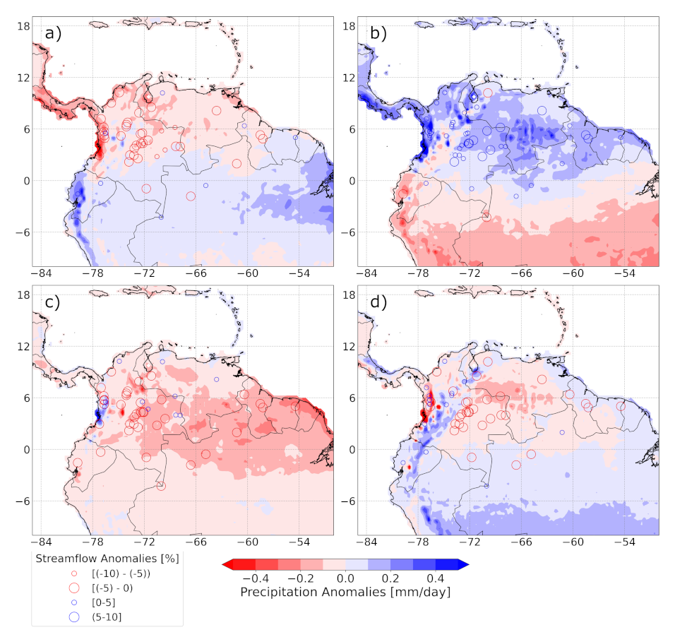
3.4. Seasonal Synoptic Anomalies

Figure 7 shows the long-term seasonal synoptic anomalies for precipitation and streamflows over the study region according to the ERA5 reanalysis for the 1981–2019 period. During DJF (Figure 7a), we observed that negative synoptic anomalies predominated over northern Colombia, Venezuela, and Central America, indicating that seasonal means were higher than 5-day seasonal means. Moreover, in southern Colombia, Ecuador, northern Peru and, northern Brazil, positive synoptic anomalies predominated, indicating that seasonal means were lower than 5-day seasonal means. In contrast, during MAM (Figure 7), the positive synoptic anomalies that appeared over the northernmost portion of South America gradually decreased and turned into negative synoptic anomalies from the Equator to $5^{\circ }$S. During JJA, the synoptic anomalies of precipitation in NSA were driven mainly by seasonal variability, except for a small portion of the far eastern Pacific coast of Colombia (Figure 7c). Finally, during SON, our results show how the positive synoptic anomalies of precipitation were located over the Andean mountain range, south of the Equator and the Guianas coast. In contrast, negative synoptic anomalies were found in northern and eastern Colombia and its western pacific coast. One striking result is that synoptic anomalies for streamflows corresponded with those found for precipitation in most catchments and seasons (circles in Figure 7). These coincidences of synoptic anomalies indicate the phasing between the atmosphere and surface processes in the catchments at synoptic time scale. Moreover, we found similar results for the CHIRPS dataset shown in the Supplementary Material (Figure S3).

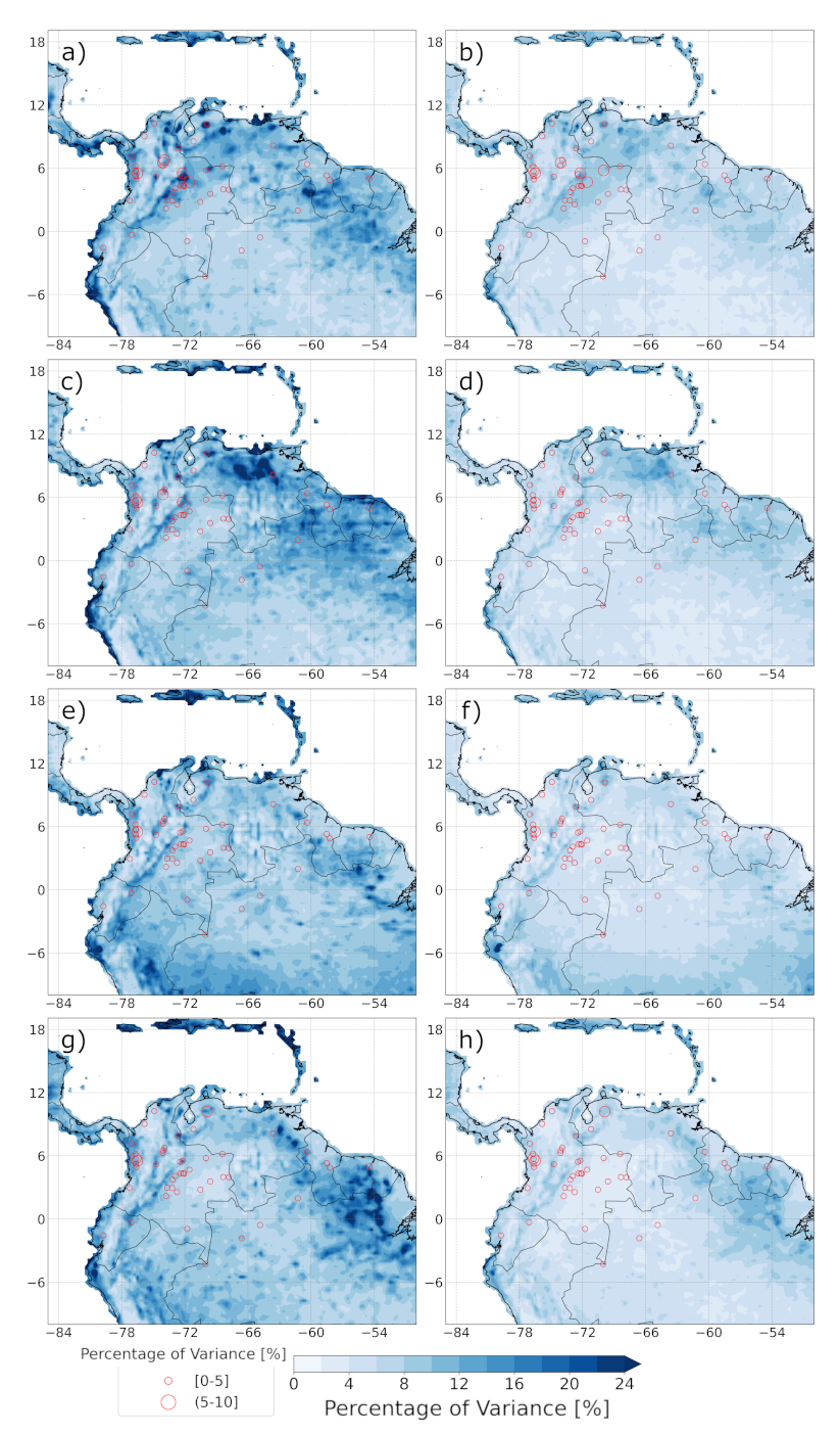
3.5. Seasonal Variance Explained by the Synoptic Modes of Variability

We quantified the seasonal percentage of variance explained by the SMV (IMF2 and IMF3) in relation to the total variance of the original time series. To that end, we used Equation (3) for DJF, MAM, JJA, and SON, respectively. This procedure allows us to associate the percentage of total variance explained by the SMV over the study region. Moreover, we computed the variance explained by other frequency bands of variability that exhibited lower frequencies than the synoptic modes. In general, the variance explained for the IMF2 showed higher values (left panels in Figure 8) than the variance explained for the IMF3 during all seasons (right panels in Figure 8).

During all trimesters, we found a high percentage of variance over the eastern flank of the Andes mountain range. Moreover, our results reveal a high variance in central Venezuela, the Guianas, northern Peru, and the western Pacific Coast of Colombia, agreeing with the regions of influence of the Kelvin waves, EWs, and MRG shown in Figure 3 and Figure S1. Furthermore, the regions that showed high seasonal variances coincided with those exhibiting high percentages of variances explained for the complete time series. Regarding those results, we highlight that JJA did not show significant differences whereas, the most notable differences appeared in the Orinoco region during DJF, central Venezuela during MAM, and Guianas during SON.

For streamflows, the higher variance explained by the SMV was found during DJF for the different flanks of the Andean mountains.

Moreover, we explored seasonal relationships between the variance and the catchment areas. Our results confirm the power fit behavior previously shown as $PV\propto A^{\theta }$ (see Figure 9). In particular, we did not find remarkable differences among the seasons using the moment ratio for IMFs 2 and 3.

4. Conclusions

This study used the ensemble empirical mode decomposition (EEMD) method to identify the synoptic mode of variability (SMV) in daily precipitation and streamflows for 47 river basins over northern South America (NSA). We found three SMVs in precipitation and streamflows. Those frequency bands can be associated with the periods 2–4 days, 3–12 days, and 6–18 days. The IMF1 is associated with a high-frequency variability that includes some synoptic contribution. In contrast, IMF2 and IMF3 are associated with synoptic variability and biweekly modes of variability that might be associated with tropical perturbations in the region, such as Kelvin waves, mixed Rossby-gravity (MRG) waves, and easterly waves (EWs), which modulate precipitation activity in the region.

We found coherence on seasonal synoptic anomalies over NSA for precipitation and streamflows. During DJF, JJA, and SON, the negative synoptic anomalies (where seasonal means were higher than 5-day seasonal means) predominated over the region comprehended between the Equator and 15${}^{\circ }$ N. In contrast, during MAM, positive synoptic anomalies (where seasonal means were lower than 5-day seasonal means) were the ones that predominated over the same region, which could be associated with the influence of the Kelvin waves over northeastern South America and the tropical north Atlantic Ocean.

Our results evidence a relevant time scale synoptic variability in precipitation and streamflows in some regions of NSA, among them: the eastern flanks of the Andean mountains, central Venezuela, Guianas, northeastern Amazon, and the western Pacific coast of Colombia. Our results for precipitation are consistent for the two gridded datasets at daily temporal resolutions used in this work (ERA5 and CHIRPS), which support the consistency and robustness of our results about synoptic time scale modes of variability in the zone of study.

Synoptic variability constituted 2.0% to 23% of the total variance of daily streamflows. In this sense, we found that the variance explained by the synoptic modes of variability in daily streamflows was higher in catchments with areas ranging from 1000 to 5000 km${}^2$ than for catchments with areas above 5000 km${}^2$. This suggests the filtering of the synoptic time variability due to processes over the area of the catchments.

5. Future Work

We investigated the SMV using the non-linear decomposition method called EEMD, whose results agree with the periods of the tropical perturbations that modulate precipitation variability in the tropics. In this sense, future work can use the methodology used here to characterize and investigate processes associated with other modes of variability at lower frequencies (e.g., intra-seasonal, annual, and inter-annual variability).

The relationship between the catchment areas and the percentage of total variability explained by the SMV for streamflows can lead to new topics for further research: (1) the role of morphometric characteristics of catchments as filters of the high-frequency atmospheric processes; (2) the importance of synoptic time scale variability in catchments with areas below 1000 km${}^2$; and (3) the role of catchments as filters of climatic processes, including frequencies different than synoptic ones.

This work on the characterization of synoptic time scale variability in daily time series of precipitation and streamflows offers procedures and results for further research and applications in hydrology and earth sciences, to (a) identify zones where the synoptic time scale variability contributes significantly to the total variability of precipitation and streamflows; (b) provide information for planning purposes that require non-real-time hydrological data at daily temporal resolution; (c) improve forecasting using autoregressive models at the daily resolution, and (d) investigate the role of catchments in the filter of significant high-frequency signals in precipitation that is not significant in streamflows.

References

1. Garreaud, R.D.; Aceituno, P. Atmospheric Circulation and Climatic Variability. In The Physical Geography of South America; Oxford University Press: Oxford, UK, 2007. [Google Scholar] [CrossRef]
2. Franzke, C.L.E.; Barbosa, S.; Blender, R.; Fredriksen, H.; Laepple, T.; Lambert, F.; Nilsen, T.; Rypdal, K.; Rypdal, M.; Scotto, M.G.; et al. The Structure of Climate Variability Across Scales. Rev. Geophys. 2020, 58, e2019RG000657. [Google Scholar] [CrossRef]
3. Mekonnen, A.; Rossow, W.B. The Interaction Between Deep Convection and Easterly Waves over Tropical North Africa: A Weather State Perspective. J. Clim. 2011, 24, 4276–4294. [Google Scholar] [CrossRef]
4. Cornforth, R.; Mumba, Z.; Parker, D.J.; Berry, G.; Chapelon, N.; Diakaria, K.; Diop-Kane, M.; Ermert, V.; Fink, A.H.; Knippertz, P.; et al. Synoptic Systems. In Meteorology of Tropical West Africa; John Wiley & Sons, Ltd.: Chichester, UK, 2017; pp. 40–89. [Google Scholar] [CrossRef]
5. Li, W.; Liu, Z.; Luo, C. Characteristics of the synoptic time scale variability over the South China Sea based on Tropical Rainfall Measuring Mission. Meteorol. Atmos. Phys. 2012, 115, 163–171. [Google Scholar] [CrossRef]
6. Wheeler, M.; Kiladis, G.N. Convectively Coupled Equatorial Waves: Analysis of Clouds and Temperature in the Wavenumber–Frequency Domain. J. Atmos. Sci. 1999, 56, 374–399. [Google Scholar] [CrossRef]
7. Kiladis, G.N.; Wheeler, M.C.; Haertel, P.T.; Straub, K.H.; Roundy, P.E. Convectively coupled equatorial waves. Rev. Geophys. 2009, 47, 1–42. [Google Scholar] [CrossRef]
8. Dias, J.; Leroux, S.; Tulich, S.N.; Kiladis, G.N. How systematic is organized tropical convection within the MJO? Geophys. Res. Lett. 2013, 40, 1420–1425. [Google Scholar] [CrossRef]
9. Agudelo, P.A.; Hoyos, C.D.; Curry, J.A.; Webster, P.J. Probabilistic discrimination between large-scale environments of intensifying and decaying African Easterly Waves. Clim. Dyn. 2011, 36, 1379–1401. [Google Scholar] [CrossRef]
10. Dominguez, C.; Done, J.M.; Bruyère, C.L. Easterly wave contributions to seasonal rainfall over the tropical Americas in observations and a regional climate model. Clim. Dyn. 2020, 54, 191–209. [Google Scholar] [CrossRef] [Green Version]
11. Jaramillo, L.; Poveda, G.; Mejía, J.F. Mesoscale convective systems and other precipitation features over the tropical Americas and surrounding seas as seen by TRMM. Int. J. Climatol. 2017, 37, 380–397. [Google Scholar] [CrossRef]
12. Zuluaga, M.D.; Houze, R.A. Extreme Convection of the Near-Equatorial Americas, Africa, and Adjoining Oceans as seen by TRMM. Mon. Weather Rev. 2015, 143, 298–316. [Google Scholar] [CrossRef] [Green Version]
13. Giraldo-Cardenas, S.; Arias, P.A.; Vieira, S.C.; Zuluaga, M.D. Easterly waves and precipitation over northern South America and the Caribbean. Int. J. Climatol. 2021. [Google Scholar] [CrossRef]
14. Brutsaert, W. Hydrology: An Introduction; Cambridge University Press: Cambridge, UK, 2005. [Google Scholar] [CrossRef]
15. Peixoto, J.P.; Oort, A.H.; Covey, C.; Taylor, K. Physics of Climate. Phys. Today 1992, 45, 67. [Google Scholar] [CrossRef]
16. Siegert, C.M.; Leathers, D.J.; Levia, D.F. Synoptic typing: Interdisciplinary application methods with three practical hydroclimatological examples. Theor. Appl. Climatol. 2017, 128, 603–621. [Google Scholar] [CrossRef]
17. Tarasova, L.; Merz, R.; Kiss, A.; Basso, S.; Blöschl, G.; Merz, B.; Viglione, A.; Plötner, S.; Guse, B.; Schumann, A.; et al. Causative classification of river flood events. WIREs Water 2019, 6, e1353. [Google Scholar] [CrossRef] [PubMed] [Green Version]
18. Hunt, K.M.; Dimri, A. Synoptic-scale precursors of landslides in the western Himalaya and Karakoram. Sci. Total Environ. 2021, 776, 145895. [Google Scholar] [CrossRef]
19. WMO. World Meteorological Organization. Meteorological Systems for Hydrological Purposes; Technical Report; WMO: Geneva, Switzerland, 2003. [Google Scholar]
20. Duchon, C.E. Lanczos Filtering in One and Two Dimensions. J. Appl. Meteorol. 1979, 18, 1016–1022. [Google Scholar] [CrossRef]
21. Salas, H.D.; Carmona, A.; Poveda, G. Variabilidad interdiaria de la precipitación en Medellín (Colombia) asociada con las ondas tropicales del este y su comportamiento durante las fases del ENSO. In Proceedings of the XXV CONGRESO LATINOAMERICANO DE HIDRÁULICA E HIDROLOGÍA, 2012; Available online: https://repositorio.unal.edu.co/handle/unal/10650 (accessed on 19 January 2022).
22. Carmona, A.M.; Poveda, G. Detection of long-term trends in monthly hydro-climatic series of Colombia through Empirical Mode Decomposition. Clim. Chang. 2014, 123, 301–313. [Google Scholar] [CrossRef]
23. Wang, W.c.; Chau, K.w.; Xu, D.m.; Chen, X.Y. Improving Forecasting Accuracy of Annual Runoff Time Series Using ARIMA Based on EEMD Decomposition. Water Resour. Manag. 2015, 29, 2655–2675. [Google Scholar] [CrossRef]
24. Wang, J.; Wang, X.; hui Lei, X.; Wang, H.; hua Zhang, X.; jun You, J.; feng Tan, Q.; lian Liu, X. Teleconnection analysis of monthly streamflow using ensemble empirical mode decomposition. J. Hydrol. 2020, 582, 124411. [Google Scholar] [CrossRef]
25. Ouyang, Q.; Lu, W.; Xin, X.; Zhang, Y.; Cheng, W.; Yu, T. Monthly Rainfall Forecasting Using EEMD-SVR Based on Phase-Space Reconstruction. Water Resour. Manag. 2016, 30, 2311–2325. [Google Scholar] [CrossRef]
26. Wu, Z.; Schneider, E.K.; Kirtman, B.P.; Sarachik, E.S.; Huang, N.E.; Tucker, C.J. The modulated annual cycle: An alternative reference frame for climate anomalies. Clim. Dyn. 2008, 31, 823–841. [Google Scholar] [CrossRef] [Green Version]
27. Wu, M.L.C.; Reale, O.; Schubert, S.D. A Characterization of African Easterly Waves on 2.5–6-Day and 6–9-Day Time Scales. J. Clim. 2013, 26, 6750–6774. [Google Scholar] [CrossRef]
28. Espinoza, J.C.; Garreaud, R.; Poveda, G.; Arias, P.A.; Molina-Carpio, J.; Masiokas, M.; Viale, M.; Scaff, L. Hydroclimate of the Andes Part I: Main Climatic Features. Front. Earth Sci. 2020, 8, 64. [Google Scholar] [CrossRef] [Green Version]
29. Arias, P.A.; Garreaud, R.; Poveda, G.; Espinoza, J.C.; Molina-Carpio, J.; Masiokas, M.; Viale, M.; Scaff, L.; van Oevelen, P.J. Hydroclimate of the Andes Part II: Hydroclimate Variability and Sub-Continental Patterns. Front. Earth Sci. 2021, 8. [Google Scholar] [CrossRef]
30. Poveda, G.; Waylen, P.R.; Pulwarty, R.S. Annual and inter-annual variability of the present climate in northern South America and southern Mesoamerica. Palaeogeogr. Palaeoclimatol. Palaeoecol. 2006, 234, 3–27. [Google Scholar] [CrossRef]
31. Ortega, G.; Arias, P.A.; Villegas, J.C.; Marquet, P.A.; Nobre, P. Present-day and future climate over central and South America according to CMIP5/CMIP6 models. Int. J. Climatol. 2021, 41, 6713–6735. [Google Scholar] [CrossRef]
32. Braz, D.F.; Ambrizzi, T.; da Rocha, R.P.; Algarra, I.; Nieto, R.; Gimeno, L. Assessing the Moisture Transports Associated With Nocturnal Low-Level Jets in Continental South America. Front. Environ. Sci. 2021, 9, 657764. [Google Scholar] [CrossRef]
33. Collins, J.M.; Chaves, R.R.; da Silva Marques, V. Temperature Variability over South America. J. Clim. 2009, 22, 5854–5869. [Google Scholar] [CrossRef] [Green Version]
34. Sörensson, A.A.; Ruscica, R.C. Intercomparison and Uncertainty Assessment of Nine Evapotranspiration Estimates Over South America. Water Resour. Res. 2018, 54, 2891–2908. [Google Scholar] [CrossRef] [Green Version]
35. Hersbach, H.; Bell, B.; Berrisford, P.; Horányi, A.; Sabater, J.M.; Nicolas, J.; Radu, R.; Schepers, D.; Simmons, A.; Soci, C.; et al. Global reanalysis: Goodbye ERA-Interim, hello ERA5. ECMWF Newsl. 2019, 159, 17–24. [Google Scholar] [CrossRef]
36. Funk, C.; Peterson, P.; Landsfeld, M.; Pedreros, D.; Verdin, J.; Shukla, S.; Husak, G.; Rowland, J.; Harrison, L.; Hoell, A.; et al. The climate hazards infrared precipitation with stations—A new environmental record for monitoring extremes. Sci. Data 2015, 2, 150066. [Google Scholar] [CrossRef] [PubMed] [Green Version]
37. Fekete, B.M.; Vörösmarty, C.J.; Grabs, W. High-resolution fields of global runoff combining observed river discharge and simulated water balances. Glob. Biogeochem. Cycles 2002, 16, 15. [Google Scholar] [CrossRef]
38. Huaman, L.; Schumacher, C.; Kiladis, G.N. Eastward-Propagating Disturbances in the Tropical Pacific. Mon. Weather Rev. 2020, 148, 3713–3728. [Google Scholar] [CrossRef]
39. Brueck, M.; Nuijens, L.; Stevens, B. On the Seasonal and Synoptic Time-Scale Variability of the North Atlantic Trade Wind Region and Its Low-Level Clouds. J. Atmos. Sci. 2015, 72, 1428–1446. [Google Scholar] [CrossRef]
40. Huang, N.E.; Shen, Z.; Long, S.R.; Wu, M.C.; Shih, H.H.; Zheng, Q.; Yen, N.C.; Tung, C.C.; Liu, H.H. The empirical mode decomposition and the Hilbert spectrum for nonlinear and non-stationary time series analysis. Proc. R. Soc. Lond. Ser. A Math. Phys. Eng. Sci. 1998, 454, 903–995. [Google Scholar] [CrossRef]
41. Huang, N.E.; Wu, Z. A review on Hilbert-Huang transform: Method and its applications to geophysical studies. Rev. Geophys. 2008, 46, RG2006. [Google Scholar] [CrossRef] [Green Version]
42. Ghil, M.; Allen, M.R.; Dettinger, M.D.; Ide, K.; Kondrashov, D.; Mann, M.E.; Robertson, A.W.; Saunders, A.; Tian, Y.; Varadi, F.; et al. Advanced spectral methods for climatic time series. Rev. Geophys. 2002, 40, 3. [Google Scholar] [CrossRef] [Green Version]
43. Rato, R.; Ortigueira, M.; Batista, A. On the HHT, its problems, and some solutions. Mech. Syst. Signal Process. 2008, 22, 1374–1394. [Google Scholar] [CrossRef] [Green Version]
44. Wu, Z.; Huang, N.E. ensemble empirical mode decomposition: A noise-assisted data analysis method. Adv. Adapt. Data Anal. 2009, 1, 1–41. [Google Scholar] [CrossRef]
45. Kammler, D.W. A First Course in Fourier Analysis; Cambridge University Press: Cambridge, UK, 2008. [Google Scholar] [CrossRef]
46. Stull, R.B. An Introduction to Boundary Layer Meteorology; Springer: Dordrecht, The Netherlands, 1988. [Google Scholar] [CrossRef]
47. Rose, C.; Smith, M.D. Mathematical Statistics with Mathematica; Springer: New York, NY, USA, 2002. [Google Scholar]
48. Frasson, R.P.d.M.; Pavelsky, T.M.; Fonstad, M.A.; Durand, M.T.; Allen, G.H.; Schumann, G.; Lion, C.; Beighley, R.E.; Yang, X. Global Relationships Between River Width, Slope, Catchment Area, Meander Wavelength, Sinuosity, and Discharge. Geophys. Res. Lett. 2019, 46, 3252–3262. [Google Scholar] [CrossRef] [Green Version]
49. Rosso, R.; Bacchi, B.; La Barbera, P. Fractal relation of mainstream length to catchment area in river networks. Water Resour. Res. 1991, 27, 381–387. [Google Scholar] [CrossRef]
50. Galster, J.C. Natural and anthropogenic influences on the scaling of discharge with drainage area for multiple watersheds. Geosphere 2007, 3, 260. [Google Scholar] [CrossRef]
51. Salazar, J.F.; Villegas, J.C.; Rendón, A.M.; Rodríguez, E.; Hoyos, I.; Mercado-Bettín, D.; Poveda, G. Scaling properties reveal regulation of river flows in the Amazon through a “forest reservoir”. Hydrol. Earth Syst. Sci. 2018, 22, 1735–1748. [Google Scholar] [CrossRef] [Green Version]
52. Poveda, G.; Vélez, J.I.; Mesa, O.J.; Cuartas, A.; Barco, J.; Mantilla, R.I.; Mejía, J.F.; Hoyos, C.D.; Ramírez, J.M.; Ceballos, L.I.; et al. Linking Long-Term Water Balances and Statistical Scaling to Estimate River Flows along the Drainage Network of Colombia. J. Hydrol. Eng. 2007, 12, 4–13. [Google Scholar] [CrossRef] [Green Version]
53. Wheeler, M.C.; Nguyen, H. Tropical Meteorology And Climate | Equatorial Waves. In Encyclopedia of Atmospheric Sciences, 2nd ed.; North, G.R., Pyle, J., Zhang, F., Eds.; Academic Press: Cambridge, MA, USA, 2015; pp. 102–112. [Google Scholar] [CrossRef]
54. Matsuno, T. Quasi-Geostrophic Motions in the Equatorial Area. J. Meteorol. Soc. Japan. Ser. II 1966, 44, 25–43. [Google Scholar] [CrossRef] [Green Version]
55. Straub, K.H.; Kiladis, G.N. Observations of a Convectively Coupled Kelvin Wave in the Eastern Pacific ITCZ. J. Atmos. Sci. 2002, 59, 30–53. [Google Scholar] [CrossRef]
56. Wheeler, M.; Kiladis, G.N.; Webster, P.J. Large-Scale Dynamical Fields Associated with Convectively Coupled Equatorial Waves. J. Atmos. Sci. 2000, 57, 613–640. [Google Scholar] [CrossRef] [Green Version]
57. Roundy, P.E.; Frank, W.M. A Climatology of Waves in the Equatorial Region. J. Atmos. Sci. 2004, 61, 2105–2132. [Google Scholar] [CrossRef]
58. Serra, Y.L.; Rowe, A.; Adams, D.K.; Kiladis, G.N. Kelvin Waves during GOAmazon and Their Relationship to Deep Convection. J. Atmos. Sci. 2020, 77, 3533–3550. [Google Scholar] [CrossRef]
59. Mayta, V.C.; Kiladis, G.N.; Dias, J.; Dias, P.L.S.; Gehne, M. Convectively Coupled Kelvin Waves Over Tropical South America. J. Clim. 2021, 34, 6531–6547. [Google Scholar] [CrossRef]
60. Andrés-Doménech, I.; García-Bartual, R.; Montanari, A.; Marco, J.B. Climate and hydrological variability: The catchment filtering role. Hydrol. Earth Syst. Sci. 2015, 19, 379–387. [Google Scholar] [CrossRef] [Green Version]
61. Molina, R.D.; Salazar, J.F.; Martínez, J.A.; Villegas, J.C.; Arias, P.A. Forest-Induced Exponential Growth of Precipitation Along Climatological Wind Streamlines Over the Amazon. J. Geophys. Res. Atmos. 2019, 124, 2589–2599. [Google Scholar] [CrossRef]
Figure 1. Location of the streamflow gauges from IDEAM, SO-HYBAM, and GRDC; the contours show the long-term daily precipitation over the study region for the period 1981–2019.
Hydrology 09 00059 g001
Figure 2. Regional wave number–frequency power spectrum of the (a) symmetric and (b) antisymmetric component of ERA5 precipitation, plotted as the ratio between raw power and the power in a smoothed red noise background spectrum (see [6] for details). Light dotted lines show the dispersion curves for the Matsuno [54] solutions to equatorially-trapped waves. Boxes represent regions of wave number–frequency filtering for the Kelvin waves, mixed Rossby-gravity (MRG) waves, and Easterly waves (EWs).
Hydrology 09 00059 g002
Figure 3. Geographical distribution of ERA5 precipitation variance for the seasons DJF (left column) and JJA (right column) for (a,b) Kelvin waves, (c,d) easterly waves (EWs), and (e,f) mixed Rossby-gravity (MRG) waves.
Hydrology 09 00059 g003
Figure 4. Fourier periodograms of precipitation and streamflows for the modes of synoptic variability according to the EEMD method in some catchments. (top row) IMFs for daily precipitation from ERA5 averaged over the catchment area. (bottom row) IMFs for daily streamflows. (a,d) IMF1, (b,e) IMF2, and (c,f) IMF3.
Hydrology 09 00059 g004
Figure 5. Percentage of the total variance explained by the synoptic modes of variability for daily precipitation over the region of study, and streamflows of each catchment (red circles). (a) IMF 1; (b) IMF 2; (c) IMF 3; (d) variance explained by the other frequency bands.
Hydrology 09 00059 g005
Figure 6. Percentage of total variance explained by the modes of synoptic variability for streamflows versus the area of the river basins. (a) IMF1; (b) IMF2; (c) IMF3; (d) variance explained by the other frequency bands.
Hydrology 09 00059 g006
Figure 7. Seasonal synoptic anomalies of precipitation (colors) and streamflows (circles), over the region of study for the period 1981–2019. (a) DJF; (b) MAM; (c) JJA; (d) SON.
Hydrology 09 00059 g007
Figure 8. Seasonal percentage of variance explained by the SMV for daily precipitation over the region of study, and streamflows over each catchment (red circles). (left column) IMF2 and (right column) IMF3. (a,b) DJF; (c,d) MAM 2; (e,f) JJA 3; (g,h) SON.
Hydrology 09 00059 g008
Figure 9. Seasonal percentages of variances explained by the IMFs for streamflows versus areas of the river basins. (Left column) IMF2 and (right column) IMF3. (a,b) DJF; (c,d) MAM; (e,f) JJA; (g,h) SON.
Hydrology 09 00059 g009