1. Introduction
Urban drainage models usually aim at supporting decisions on flooding mitigation, pollution control, sewer system management and, increasingly, city planning and regeneration [
1,
2,
3]. Depending on the objectives of the work and the availability of hydrological and asset data, the models can be either distributed and physically based or more aggregated and conceptual [
4,
5,
6,
7]. The increasing implementation of decentralized measures and nature-based solutions, i.e., solutions that seek to replicate natural phenomena across the catchment, often requires distributed models and, in some cases, more detailed modelling of infiltration, evapotranspiration and water quality [
8,
9].
Calibration requirements also depend on the objectives of the study, the availability of data and the time and resources needed to collect data [
10]. Calibration tends to be more demanding and conservative for the variables and scales most relevant for the study purpose. For example, in a model developed for flood risk assessment, emphasis is put on calibrating peak flows of the most severe storms [
11,
12], while in a model designed to manage combined sewer overflows (CSO), greater accuracy is required in calibrating the volumes of hydrographs for a much wider range of events, which includes medium and small magnitude rainfall [
13,
14,
15]. In the latter case in particular, daily and seasonal variations in dry weather flow [
16] and rainfall derived infiltration and inflow (RDII) may play a very important role [
17,
18,
19,
20,
21].
The number of rain events recommended for calibration and verification and the representativeness of the monitored events also depend on the objectives for which the model was designed [
22]. However, it is common that models developed for a particular purpose are later used for other analyses with a broader scope than the one for which they were initially validated.
Uncertainty in hydrological modelling derives from several sources: observed data used to force and calibrate the model (measurement); model structure, which includes errors in the mathematical formulation that represents the hydrological phenomena; parameterization; and initial and boundary conditions. Parameterization uncertainty results from both structural and measurement uncertainties, the need to conceptually simplify processes, and the inability to estimate and measure the temporal and spatial variability of the effective parameters, among others [
23,
24,
25,
26,
27].
Several methods have been used to analyse the uncertainty of hydrological models, although only a few have the ability to address, in an explicit and cohesive way, the three critical aspects of uncertainty analysis: understanding, quantification and uncertainty reduction [
24]. One of the widely used methods is the generalized likelihood uncertainty estimation (GLUE), although it depends on subjective choices and lacks a formal statistical basis [
25]. Of the various developments in formal Bayesian approaches, the most current that has been widely used is the differential evolution adaptive metropolis (DREAM), which merges the differential evolution algorithm with the adaptive Markov Chain Monte Carlo (MCMC) approach [
25]. Machine learning and polynomial chaos expansion are other approaches based on data-driven uncertainty quantification that have recently experienced increasing development [
16,
28,
29,
30]. These methods make it possible to quantify uncertainty, determine error confidence intervals and, in the case of formal Bayesian approaches, reduce the parameter uncertainty by the inclusion of prior knowledge. Despite their advantages, these methods are complex, require expert-knowledge and a high computational effort, some have convergence issues and others depend on subjective decisions [
24,
25].
For most cases, the most practical and viable way to assess uncertainty is to quantify the goodness-of-fit or accuracy of model results in measured data, for which several statistical and graphical techniques have been used, developed and discussed [
31,
32,
33,
34,
35,
36,
37,
38,
39,
40,
41,
42,
43]. An open source library with over 60 metrics recently implemented in Python and MATLAB
® is presented in [
44].
In practice, only about a dozen statistical metrics have been commonly used in hydrology, which can be classified into three main categories [
36]: dimensionless (e.g., the widely used Nash–Sutcliffe Efficiency coefficient [
31]); error index (e.g., the root mean square error); standard regression. It is consensual that both graphical techniques and more than one quantitative statistics should be used in model evaluation [
33,
36,
39]. The Nash–Sutcliffe Efficiency coefficient has been by far the most used.
The most widely applied metrics do not take into account measurement errors, although modifications to some of them have been proposed to account for measurement uncertainty [
35] and, later, for both measurement and simulation uncertainties [
38].
Based on results reported in the literature, from watershed-scale models and for annual, monthly and daily temporal scales, Moriasi et al. (2007) [
36] proposed thresholds for various dimensionless performance metrics according to qualitative ratings: “Very Good”, “Good”, “Satisfactory” and “Unsatisfactory”. These thresholds were reviewed in Moriasi et al. (2015) [
39], although the previous thresholds continue to be widely cited in the literature.
Despite the obvious advantages of this benchmarking, some authors call the attention to the drawbacks of the ad hoc use of aggregated efficiency metrics and to the greater need for modellers to understand the suitability of each metric and how it should be interpreted for the purposes of each model [
45].
Obviously, in urban drainage, graphical and statistical techniques have always been applied to model calibration and evaluation, although the generalized use of aggregated efficiency metrics, such as the Nash–Sutcliffe coefficient and the Kling-Gupta coefficient [
37], is more recent (e.g., [
46,
47,
48,
49,
50,
51,
52,
53,
54,
55]).
However, the temporal and spatial scales of urban catchments and the issues related to wet weather discharges (from both CSO and Sanitary Sewer Overflows, SSO) pose challenges that have not yet been sufficiently discussed, in particular when adopting thresholds for performance ratings proposed on the basis of other realities. The variability of the dry weather flow and the RDII can substantially contribute to the uncertainty of the model results concerning CSO and SSO discharges (CSO structures are usually designed to carry 3 to 6 times the average daily dry weather flow to the wastewater treatment plant). In these cases, the traditional approach of removing base flows to calibrate or assess the accuracy of the hydrological model becomes particularly difficult and debatable.
This article presents a brief description and discussion in the light of urban drainage of the most used metrics for model calibration and quality assessment, which are then applied to small urban catchment models with different levels of performance. An innovative approach more suited to the challenges of these catchments is proposed and the results are discussed in detail.
3. Challenges from Short-Duration Peak Flows in the Application of Metrics
The NSE, KGE and error statistics are commonly used to compare time series between modelled and observed values. However, in small urban and natural catchments, including ephemeral streams [
57,
58], many significant peak flows occur during very short periods of time. The spatial variability of rainfall and small desynchronizations between rain and flow measurement equipment can lead to delays or advances of the modelled series in relation to the observed series of only a few minutes, but with a significant impact on the statistical results.
Figure 2 shows the measured and modelled hydrographs of the most intense storm monitored in the case study presented below.
Table 1 compares the results of the statistics described in the previous section for four scenarios: (a) the case represented in
Figure 2; (b) the measured flow rate advanced by 2 min; (c) the measured flow rate delayed by 4 min; and (d) measured flow delayed by 6 min.
According to the results in
Table 1, scenario (b) is the one that leads to the best results, with values of NSE, KGE, slope and coefficient of determination very close to the unity. However, NSE is less than 0.5 and 0.35 for scenarios (c) and (d), respectively, with only 4 and 6 min of rainfall delay. The error values also rise significantly for scenarios (c) and (d).
These results highlight the significant impact that small time deviations between measured and simulated series can have on the results of various metrics.
4. Materials and Methods
4.1. The Proposed New Approach
In a context of an increasingly widespread adoption of decentralized and nature-based solutions, the measures to be modelled will influence the entire urban water cycle, covering small to heavy rainfall. Therefore, assessing the shape of hydrographs for a wide range of rainfall events is of great importance. In order to strengthen the assessment of the shape of hydrographs and reduce the inconveniences of the event-by-event analysis described above, a new approach is proposed to assess the quality of hydrological models.
Rather than the performance metrics being applied to compare measured and simulated values within each hydrograph (and/or the measured and simulated peak flows of the various hydrographs), they could be applied to compare measured and simulated maximum flows for various durations. For each duration, the measured and simulated maximum flow series can be easily calculated by applying a rolling-window search routine to each hydrograph.
Hence, the assessment of model results is performed simultaneously for a pre-selected set of durations from all hydrographs. To avoid excessive complexity in the analysis, it is important to use a limited but representative number of durations, so we recommend selecting five to eight durations with increasing intervals between them. For the case study presented below, the maximum flow rates associated with the following durations will be assessed: 2, 6, 16, 30, 60, 104 and 150 min.
Table 2 presents an example of the application of the metrics described in
Section 2 to the durations selected in the case study, according to the proposed approach. In addition to numerical metrics, graphical techniques must also be applied, as mentioned above and will be presented in the case study.
By evaluating peak flows for a wide range of durations, this new approach favours the assessment of the shape of hydrographs, as well as the effect of the uncertainty of both base flows and CSO discharges.
This new approach will be applied to assess eight different models (or modelling conditions) of the case study.
4.2. Case Study
The study area is located at Odivelas, a 26.5 km2 municipality of the Lisbon Metropolitan Area, Portugal, and is 102 ha in size. It consists of two distinct catchments: a combined catchment, with 22 ha, of which the main sewer receives the foul flow from a 400 mm upstream interceptor sewer; a mixed and partially separate catchment upstream, with about 80 ha, served by the mentioned interceptor sewer. For wet weather, the interceptor sewer transports a mixture of wastewater and stormwater, sometimes under pressure.
The two catchments have mainly a residential occupation with some commerce. In the downstream combined catchment, most sewers are built of concrete (Manning coefficient of 0.014 s·m−1/3) and have a circular cross-section of 300 and 400 mm, increasing up to 1000 mm downstream. The sewer slopes are close to those of the terrain, ranging from 0.3 to 11% and with a mean and median of 2.8% and 2.3%, respectively. The percentages of paved, roofed and green areas are 46%, 35%, and 19%, respectively. However, only about 70% of the runoff from impermeable areas drains into the sewer network, due to drainage to backyards and the insufficient number of inlet devices.
Over a decade ago, the downstream combined catchment was modelled in detail using the Stormwater Management Model (SWMM) [
59], with 86 sub-catchments, 145 nodes and 153 sewer branches. However, the drainage system of the upstream mixed catchment is complex and is not known in detail, so it was modelled in an aggregated way using SWMM, considering only the two main combined sewer overflows (CSO) and two sub-catchments, with 68 ha and 12 ha (
Figure 3).
For both catchments, the model was calibrated and verified on basis of data from a 4-month monitoring survey, in which 26 rainfall events were recorded by two rain gauges and two flowmeters. One flow meter was installed in the interceptor sewer, a few meters upstream of the entrance to the combined catchment (section B1-I), and the other was installed downstream from the combined catchment (section B1-M).
The peak flow of the most intense monitored event reached 80% of the maximum capacity of the combined system, of 1530 L/s, in a sewer downstream B1-M (and 60% of the capacity in B1-M, which already has a maximum diameter of 1 m). Downstream B1-M, the sewer is under pressure for return periods greater than 2–5 years and flooding occurs for return periods greater than 5–10 years.
As the complexity of the upstream catchment behavior did not allow us to obtain good calibration and verification results in the section B1-I, part of the underestimation of the flows in the interceptor sewer was compensated by some overestimation of the flows in the downstream combined catchment, allowing us to obtain very good results in B1-M. Thus, the model was left with a “black box” component inside, but it was quite adequate for the purpose of the study at the time. The model was used to evaluate the CSO discharges from the downstream catchment, both by event-by-event analyses [
60,
61] and using a 19-year rainfall historical series [
62,
63].
Currently, the model is intended to be used to study stormwater management measures distributed within the combined catchment, with a view to reduce CSO discharges, mitigate floods and improve the urban water cycle. Therefore, it is important to improve the calibration of the upstream aggregated model (modelled with only the two main CSO and two sub-catchments) and, hence, to model more accurately the flows generated in the combined catchment downstream. Between sections B1-I and B1-M there is a small CSO structure that shaves off the highest flows measured in B1-I, which could not be monitored and has not been modelled in the past. This CSO adds complexity to the model and its calibration requires a detailed quantification of the shape of the hydrographs in B1-I and B1-M.
The variability of base flows during rainfall events also plays an important role both in the estimation of the wet weather overflow discharges and in the calibration of this CSO structure.
Figure 4 shows the hourly variation of the average and median flow (Qav and Qmedian) for the weekdays, as well as the 10th, 25th, 75th and 90th percentiles (Q10, Q25, Q75 and Q90). The horizontal lines represent the same statistics for the daily flows.
As
Figure 4 shows, there is substantial variability in the daily dry weather flows, particularly in the downstream section. This variability is attributed to three main factors: the activities in the catchment; the groundwater infiltration into the sewers, although there is not a sufficiently long series to make it possible to model the RDII component; as well as to the measurement error, which significantly depends on the cleanliness and the accumulation of debris on the submerged pressure and velocity gauges.
4.3. Model Recalibration and Verification
Nine from the 26 events were selected for the sensitivity analysis of the parameters and for the recalibration of the models: events 1, 4, 7, 9, 13, 16, 19, 21 and 24. The selected events include five of the eight events that led to flow rates above the discharge threshold of the CSO structure located between sections B1-I and B1-M.
The other 17 events were used to verify the models.
The recalibration of the partially separate upstream catchment consisted mainly of adjusting the contributing areas of the two sub-catchments and the flow capacity of the respective CSO structures. The recalibration of the downstream catchment consisted mainly of calibrating the discharge capacity of the CSO structure between B1-I and B1-M, adjusting the impermeable area and improving the shape of the hydrographs, through the slope and width of the sub-catchments.
Calibration was carried out manually based on volumes, peak flows and the shape of the hydrographs.
All 26 events were used to assess the quality of the models based on the proposed new approach described in
Section 4.1, given that only five calibration and three verification events led to discharges in all CSO structures.
However, during the quality assessment of the global model in B1-M by the proposed approach and using the 26 events, it was determined that a small correction to the shape of the hydrographs should be done by increasing the slope and the width of the catchments and slightly decreasing the contribution of the impervious area. Hence, the set of 26 events was initially used to assess the quality of the model and later to enhance the calibration.
If the monitored stormwater event set were large enough that it could be split into two representative subsets of at least 20 events each, it would be recommended to split it into two subsets, one for model calibration and one for verification.
Performance metrics were applied to all rainfall events, but the results were substantially influenced by the time lags between the measured and modelled hydrographs, as described in
Section 3. No attempt was made to synchronize the simulated and measured hydrographs, due to the subjectivity this would introduce. These results are presented in
Table A1 and
Table A2 of
Appendix A and will be discussed in
Section 5.4.
4.4. Application of the Proposed New Approach
The new approach described in
Section 4.1 was applied to eight quality assessments of case study models.
For both monitoring sections B1-I and B1-M, three assessments were carried out, two to evaluate the quality of the initial and recalibrated models, in which the dry weather flow (DWF) is adjusted event by event, and the third to evaluate the accuracy of the recalibrated model results without DWF adjustment.
For the downstream monitoring section B1-M, two additional assessments were carried out: one with a recalibrated model of the upstream interceptor sewer catchment, but still with the initial model of the downstream combined catchment (with adjustment of DWF); and another with the model recalibrated downstream, but receiving from the interceptor sewer the inflows measured in B1-I (with the DWF adjusted only in B1-M).
Table 3 lists the order in which the results of the eight assessments will be presented and discussed in the next section.
6. Conclusions
Small urban catchments pose challenges in applying performance metrics when comparing measured and simulated hydrographs. Indeed, results are hampered by the short peak flows, due to rainfall variability and measurement synchronization errors, and it can be both difficult and inconvenient to remove base flows from the analysis, given their influence on the performance of CSO structures. In addition, base flows are an important source of uncertainty in modelling small rainfall events, which must be taken into account when assessing the quality of the models.
A new approach was proposed and tested to assess the quality of models of small combined catchments, which proved to be quite suitable not only for the assessment of the quality of the models, but also to support calibration. In the proposed approach, rather than the performance metrics being applied to compare the measured and simulated values within each hydrograph and/or the measured and simulated peak flows of the various events, they are applied to compare measured and simulated maximum flows for a set of different durations. For each duration, the measured and simulated maximum flow series can be easily calculated by applying a rolling-window search routine to each hydrograph. To keep the assessment simple, five to eight different durations with increasing intervals should be analysed.
This new approach presents the following advantages: (a) being simple; (b) avoiding the inconveniences arising from the time lags of very short peaks (described in
Section 3) and the subjectivity of possible adjustments; (c) favouring the assessment of the influence of base flow and RDII variability (see assessments C2, C3 and C7) and the influence of peak flow shaving by upstream CSOs (assessment C5); (d) promoting and facilitating an integrated analysis for a wide range of rainfall events; (e) avoiding subjectivity in interpreting different results for the various events; and (f) making it possible to identify biases in simulated hydrographs that would otherwise be difficult to detect, also guiding calibration.
However, it has the disadvantage of requiring a sufficiently large and representative set of rainfall events to ensure statistical significance, which, in principle, should not be less than 20 events for evaluating the quality of model results or twice that number for a complete model calibration and verification.
In addition, the results delivered by this new approach should not be compared with the thresholds proposed in Moriasi et al. (2015) [
39] without careful consideration, as the values of NSE, r
2 and PBIAS tend to be closer to optimal values than when applying metrics to compare measured and simulated values within each hydrograph.
This recommendation is extended to all modelers who apply performance metrics to peak flows in urban drainage systems.
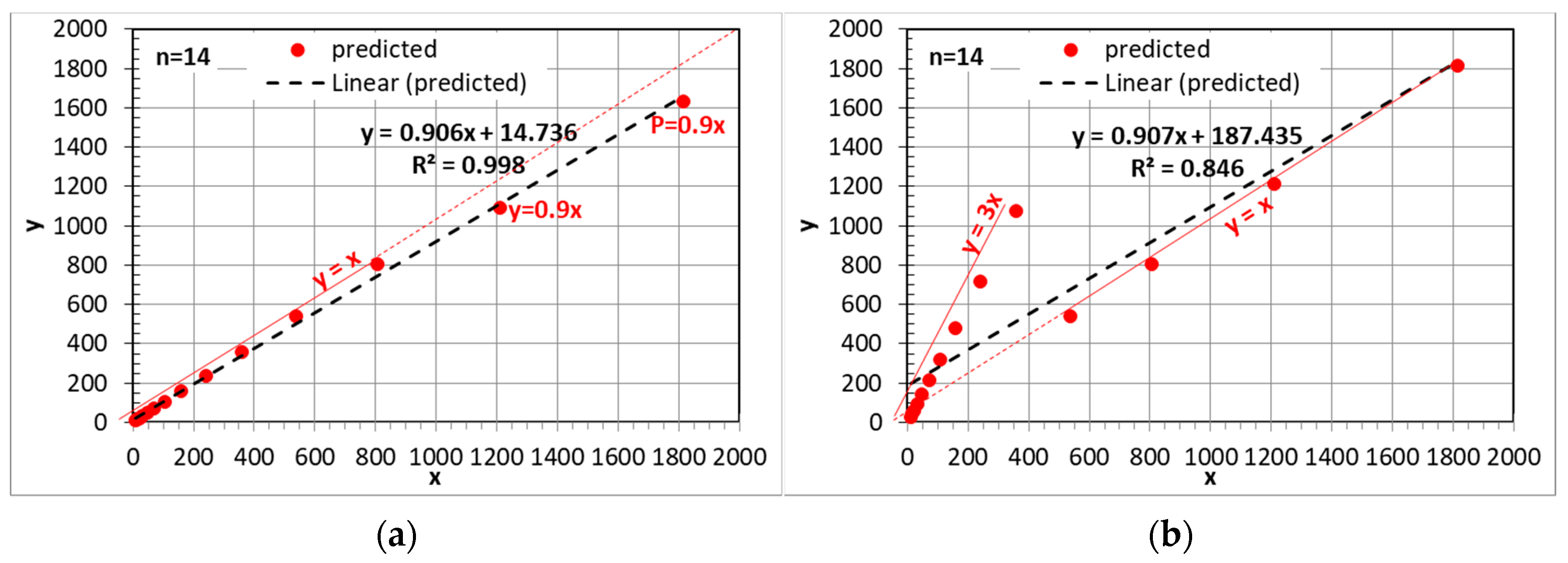
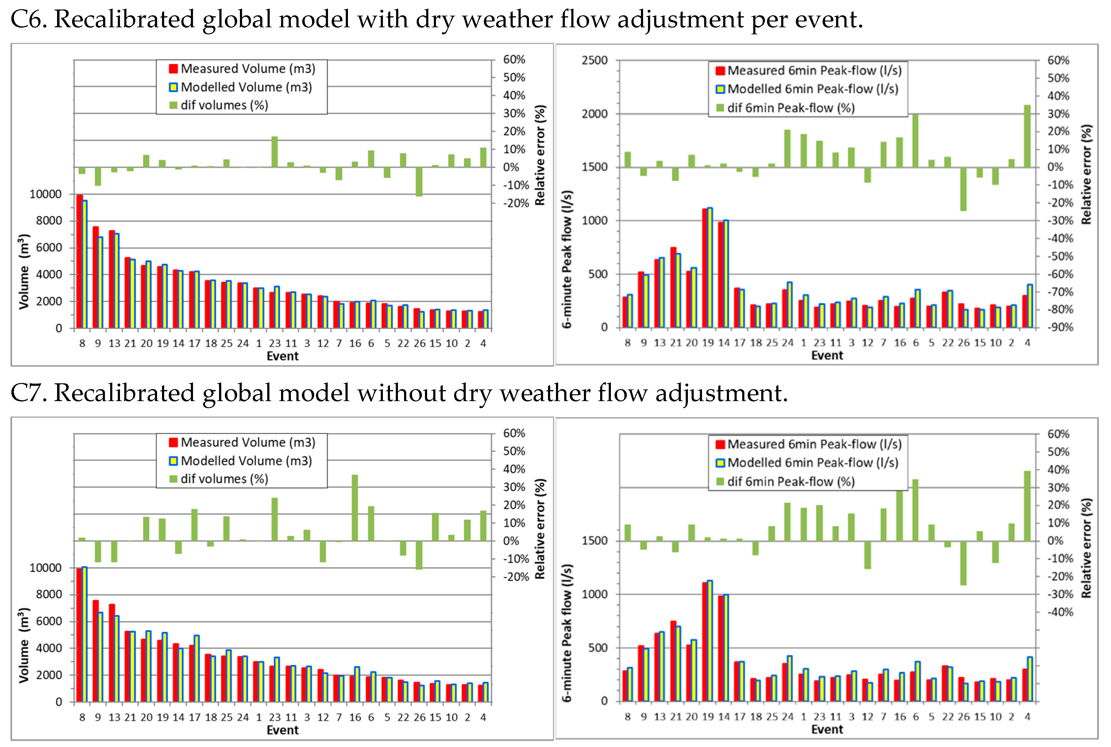
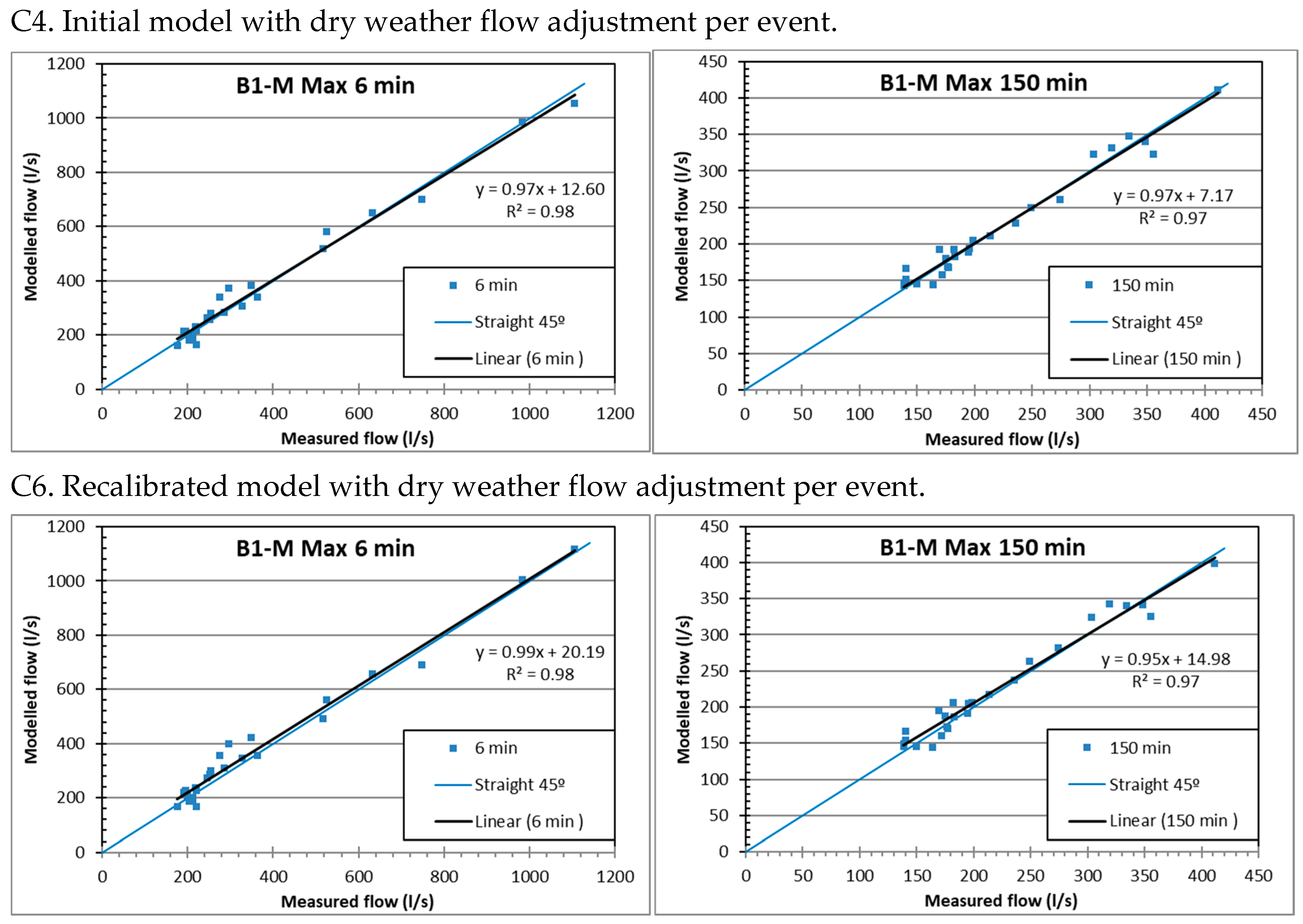
In the application of the described new approach to a model classified as providing a useful but limited and underestimated approximation (assessment C1), the NSE values were below 0.8 for all durations and, for some, below 0.7. KGE values ranged from 0.7 to 0.85. PBIAS values were less than ±10%. For the recalibrated model, providing results that tend to be good but with deviations and limitations for some events (assessment C2), the NSE values tended to be greater than 0.8, the KGE values tended to approach 0.9 and PBIAS were within ±5%. Finally, for models of which the simulated and measured hydrographs are very coincident for some events and show small deviations in other events (assessments C4 and C6), both the NSE and the KGE values were higher than 0.95 for all durations, reaching 0.98 and 0.99 in some cases.
During normal use of the model, base flows are unknown. Without adjusting base flows (assessments C3 and C7), NSE values tended to fall by up to 0.1, depending on duration, while KGE values tended to vary much less. For the “very good” quality model (assessments C7 compared with C6), the RMSE values increased between 20% and 50% as the analysed duration increased to 150 min, due to the influence of the unmodelled RDII.
The various examples of the case study highlight the importance of using different metrics and graphical analyses and the pertinence of the proposed approach.


