

Developing Patient-Specific Statistical Reconstructions of Healthy Anatomical Structures to Improve Patient Outcomes


Abstract
1. Introduction
2. Materials and Methods
2.1. Anatomical Data Description
2.2. Standardized Data Processing
2.3. Anatomical Data from Damaged Structures
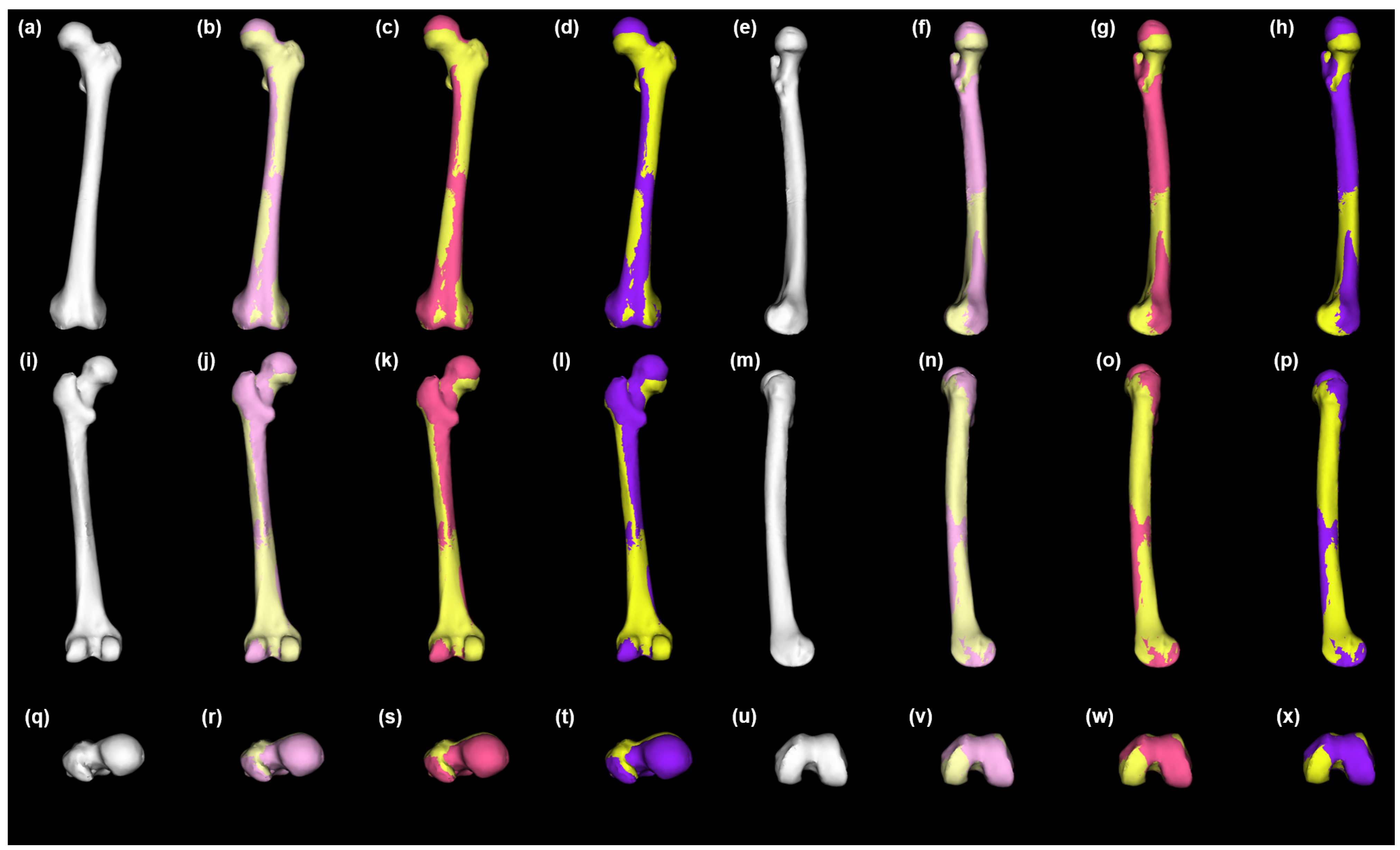
2.4. Statistical Shape Model Generation
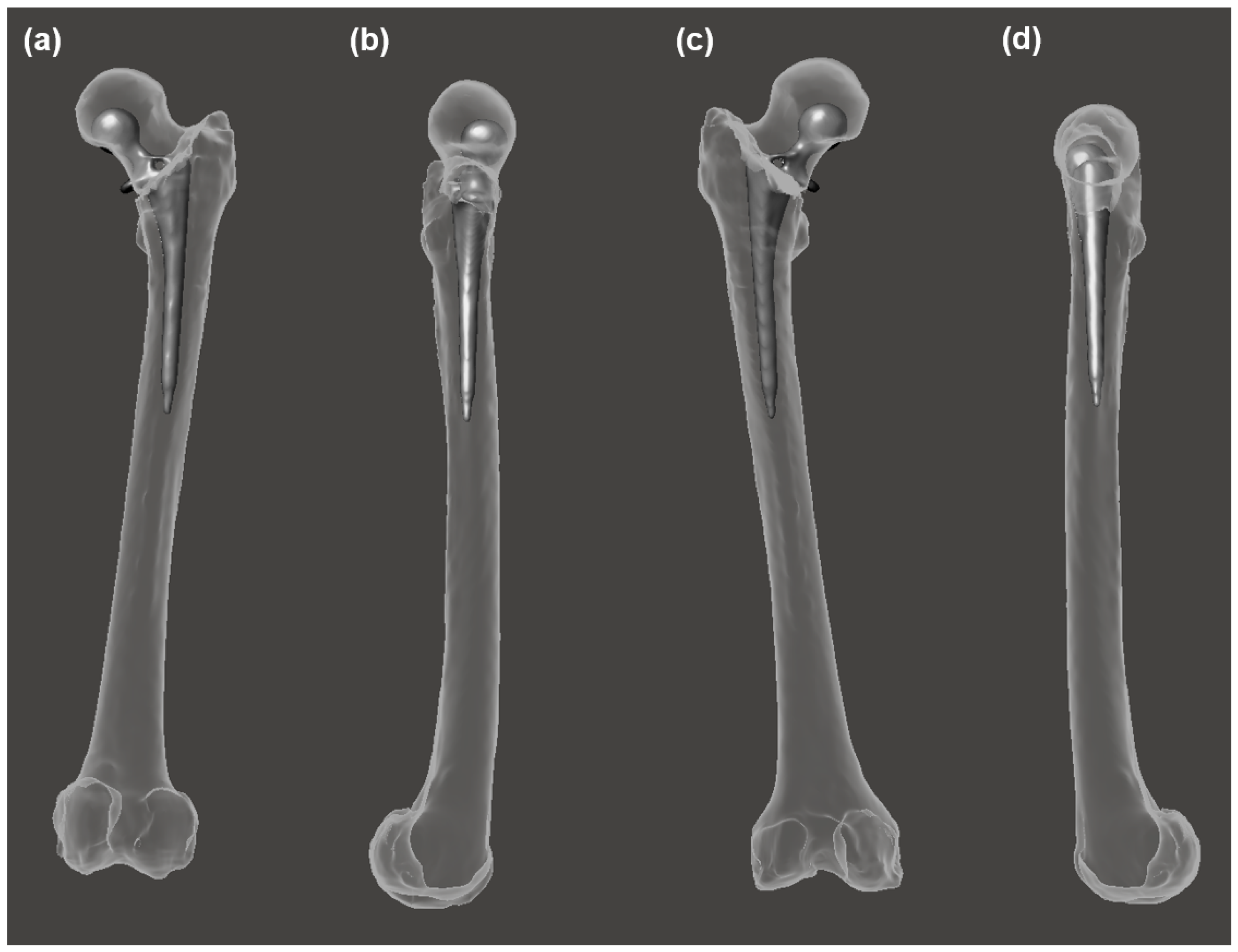
2.5. Statistical Reconstruction of Healthy Anatomy
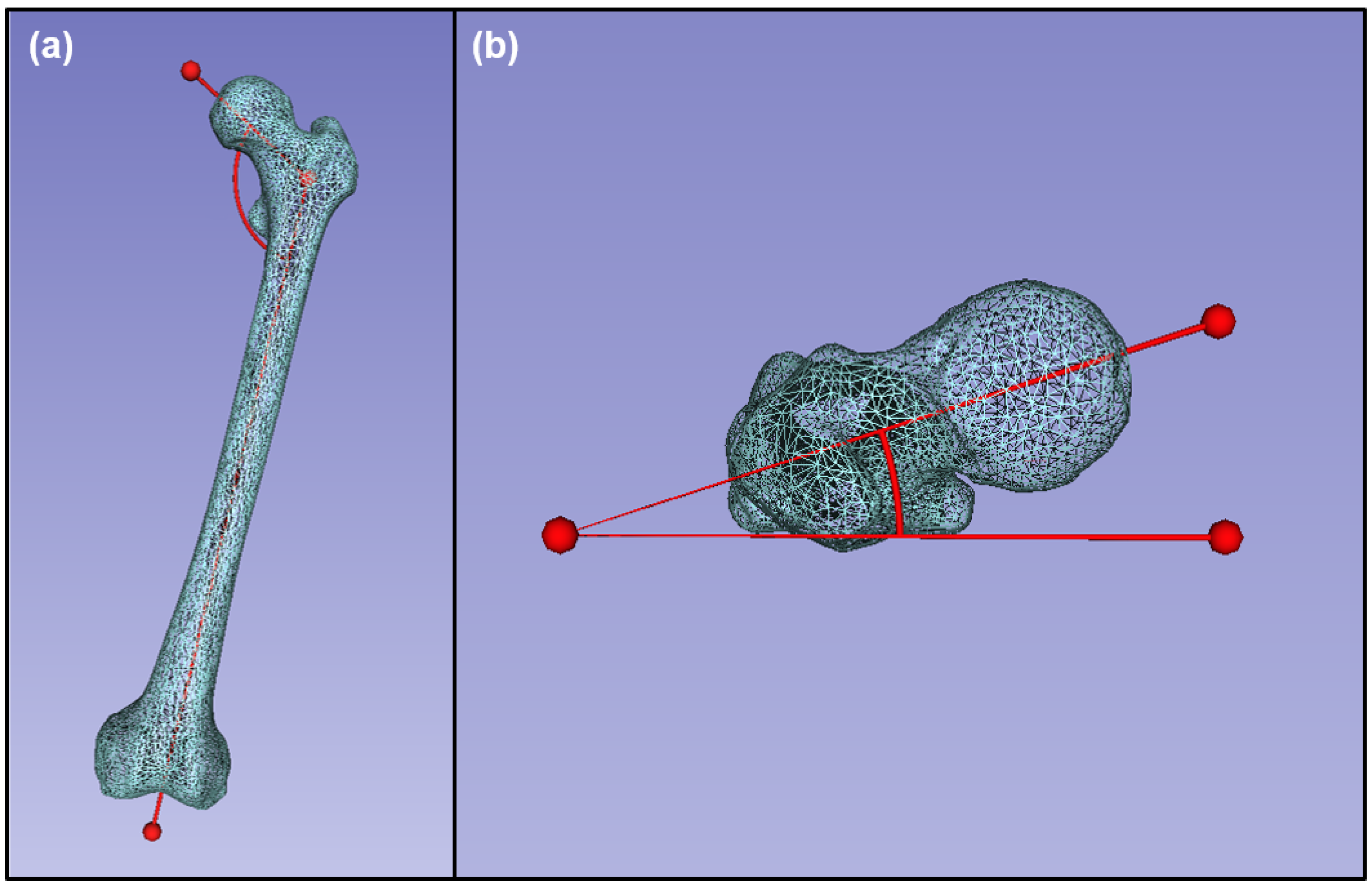
2.6. Morphological Data Collection
3. Results
4. Discussion
5. Conclusions
Author Contributions
Funding
Institutional Review Board Statement
Informed Consent Statement
Data Availability Statement
Acknowledgments
Conflicts of Interest
Abbreviations
| CT | Computed Tomography |
| SSM | Statistical Shape Model |
| UB | University at Buffalo |
| CTRC | Clinical and Translational Research Center |
| ICP | Iterative Closest Points |
| PCA | Principal Component Analysis |
| GP | Gaussian Process |
| SD | Standard Deviation |
| StatRecon | Statistical Reconstructions |
| FNA | Femoral Neck Anteversion |
| NSA | Neck-Shaft Angle |
| TrPr | Traditional Prosthesis |
References
- Pivec, R.; Johnson, A.J.; Mears, S.C.; Mont, M.A. Hip arthroplasty. Lancet 2012, 380, 1768–1777. [Google Scholar] [CrossRef] [PubMed]
- Karachalios, T.; Komnos, G.; Koutalos, A. Total hip arthroplasty: Survival and modes of failure. EFORT Open Rev. 2018, 3, 232–239. [Google Scholar] [CrossRef]
- Dobzyniak, M.; Fehring, T.K.; Odum, S. Early failure in total hip arthroplasty. Clin. Orthop. Relat. Res. 2006, 447, 76–78. [Google Scholar] [CrossRef]
- Berger, R.; Kull, L.; Rosenberg, A.; Galante, J. Hybrid total hip arthroplasty: 7- to 10-year results. Clin. Orthop. Relat. Res. 1996, 333, 134–146. [Google Scholar] [CrossRef]
- Engh, C.A., Jr.; William, J.; Culpepper, I.; Engh, C.A. Long-term results of use of the anatomic medullary locking prosthesis in total hip arthroplasty. JBJS 1997, 79, 177–184. [Google Scholar] [CrossRef]
- Ferguson, R.J.; Palmer, A.J.; Taylor, A.; Porter, M.L.; Malchau, H.; Glyn-Jones, S. Hip replacement. Lancet 2018, 392, 1662–1671. [Google Scholar] [CrossRef]
- Dy, C.J.; Bozic, K.J.; Pan, T.J.; Wright, T.M.; Padgett, D.E.; Lyman, S. Risk factors for early revision after total hip arthroplasty. Arthritis Care Res. 2014, 66, 907–915. [Google Scholar] [CrossRef]
- Pramanik, S.; Agarwal, A.K.; Rai, K. Chronology of total hip joint replacement and materials development. Trends Biomater. Artif. Organs 2005, 19, 15–26. [Google Scholar]
- Vanrusselt, J.; Vansevenant, M.; Vanderschueren, G.; Vanhoenacker, F. Postoperative radiograph of the hip arthroplasty: What the radiologist should know. Insights Imaging 2015, 6, 591–600. [Google Scholar] [CrossRef]
- Brand, R.A.; Mont, M.A.; Manring, M. Biographical sketch: Themistocles Gluck (1853–1942). Clin. Orthop. Relat. Res. 2011, 469, 1525–1527. [Google Scholar] [CrossRef]
- Knight, S.R.; Aujla, R.; Biswas, S.P. Total Hip Arthroplasty-over 100 years of operative history. Orthop. Rev. 2011, 3. [Google Scholar]
- Hopley, C.; Stengel, D.; Ekkernkamp, A.; Wich, M. Primary total hip arthroplasty versus hemiarthroplasty for displaced intracapsular hip fractures in older patients: Systematic review. BMJ 2010, 340. [Google Scholar] [CrossRef] [PubMed]
- Muster, D. Themistocles Gluck, Berlin 1890: A pioneer of multidisciplinary applied research into biomaterials for endoprostheses. Bull. History Dent. 1990, 38, 3–6. [Google Scholar]
- Eynon-Lewis, N.; Ferry, D.; Pearse, M. Themistocles Gluck: An unrecognised genius. BMJ 1992, 305, 1534. [Google Scholar] [CrossRef]
- Lugli, T. Artificial shoulder joint by Péan (1893): The facts of an exceptional intervention and the prosthetic method. Clin. Orthop. Relat. Res. 1978, 133, 215–218. [Google Scholar]
- Charnley, J. Arthroplasty of the hip: A new operation. Lancet 1961, 277, 1129–1132. [Google Scholar] [CrossRef]
- Wiles, P. The surgery of the osteo-arthritic hip. Br. J. Surg. 1958, 45, 488–497. [Google Scholar] [CrossRef]
- Ninh, C.C.; Sethi, A.; Hatahet, M.; Les, C.; Morandi, M.; Vaidya, R. Hip dislocation after modular unipolar hemiarthroplasty. J. Arthroplast. 2009, 24, 768–774. [Google Scholar] [CrossRef]
- Woo, R.Y.; Morrey, B.F. Dislocations after total hip arthroplasty. J. Bone Jt. Surg. Am. 1982, 64, 1295–1306. [Google Scholar] [CrossRef]
- Bierbaum, B.E.; Nairus, J.; Kuesis, D.; Morrison, J.C.; Ward, D. Ceramic-on-ceramic bearings in total hip arthroplasty. Clin. Orthop. Relat. Res. 2002, 405, 158–163. [Google Scholar] [CrossRef]
- Sandhu, H.S.; Middleton, R.G. Controversial topics in orthopaedics: Ceramic-on-ceramic. Ann. R. Coll. Surg. Engl. 2005, 87, 415. [Google Scholar] [PubMed]
- Wilson, L.F.; Nolan, J.F.; Heywood-Waddington, M. Fracture of the femoral stem of the Ring TCH hip prosthesis. J. Bone Jt. Surg. Am. 1992, 74, 725–728. [Google Scholar] [CrossRef]
- Gwam, C.U.; Mistry, J.B.; Mohamed, N.S.; Thomas, M.; Bigart, K.C.; Mont, M.A.; Delanois, R.E. Current epidemiology of revision total hip arthroplasty in the United States: National Inpatient Sample 2009 to 2013. J. Arthroplast. 2017, 32, 2088–2092. [Google Scholar] [CrossRef] [PubMed]
- Bernstein, M.; Walsh, A.; Petit, A.; Zukor, D.J.; Antoniou, J. Femoral head size does not affect ion values in metal-on-metal total hips. Clin. Orthop. Relat. Res. 2011, 469, 1642–1650. [Google Scholar] [CrossRef]
- Suri, M.S.M.; Hashim, N.L.S.; Syahrom, A.; Latif, M.J.A.; Harun, M.N. Influence of dimple depth on lubricant thickness in elastohydrodynamic lubrication for metallic hip implants using fluid structure interaction (FSI) approach. Mal. J. Med. Health Sci. 2020, 16, 28–34. [Google Scholar]
- Jamari, J.; Ammarullah, M.I.; Santoso, G.; Sugiharto, S.; Supriyono, T.; Prakoso, A.T.; Basri, H.; van der Heide, E. Computational Contact Pressure Prediction of CoCrMo, SS 316L and Ti6Al4V Femoral Head against UHMWPE Acetabular Cup under Gait Cycle. J. Funct. Biomater. 2022, 13, 64. [Google Scholar] [CrossRef] [PubMed]
- Vogel, D.; Klimek, M.; Saemann, M.; Bader, R. Influence of the Acetabular Cup Material on the Shell Deformation and Strain Distribution in the Adjacent Bone—A Finite Element Analysis. Materials 2020, 13, 1372. [Google Scholar] [CrossRef] [PubMed]
- Saputra, E.; Budiwan Anwar, I.; Jamari, J.; Heide, E.v.d. Reducing Contact Stress of the Surface by Modifying Different Hardness of Femoral Head and Cup in Hip Prosthesis. Front. Mech. Eng. 2021, 7, 631940. [Google Scholar] [CrossRef]
- Ammarullah, M.I.; Afif, I.Y.; Maula, M.I.; Winarni, T.I.; Tauviqirrahman, M.; Akbar, I.; Basri, H.; van der Heide, E.; Jamari, J. Tresca stress simulation of metal-on-metal total hip arthroplasty during normal walking activity. Materials 2021, 14, 7554. [Google Scholar] [CrossRef]
- Chethan, K.; Shyamasunder Bhat, N.; Satish Shenoy, B. Biomechanics of hip joint: A systematic review. Int. J. Eng. Technol. 2018, 7, 1672–1676. [Google Scholar]
- Ammarullah, M.I.; Santoso, G.; Sugiharto, S.; Supriyono, T.; Wibowo, D.B.; Kurdi, O.; Tauviqirrahman, M.; Jamari, J. Minimizing risk of failure from ceramic-on-ceramic total hip prosthesis by selecting ceramic materials based on tresca stress. Sustainability 2022, 14, 13413. [Google Scholar] [CrossRef]
- Jamari, J.; Ammarullah, M.I.; Saad, A.P.M.; Syahrom, A.; Uddin, M.; van der Heide, E.; Basri, H. The effect of bottom profile dimples on the femoral head on wear in metal-on-metal total hip arthroplasty. J. Funct. Biomater. 2021, 12, 38. [Google Scholar] [CrossRef] [PubMed]
- Ammarullah, M.I.; Santoso, G.; Sugiharto, S.; Supriyono, T.; Kurdi, O.; Tauviqirrahman, M.; Winarni, T.I.; Jamari, J. Tresca stress study of CoCrMo-on-CoCrMo bearings based on body mass index using 2D computational model. J. Tribol. 2022, 33, 31–38. [Google Scholar]
- Chethan, K.; Zuber, M.; Shyamasunder Bhat, N.; Satish Shenoy, B. Optimized trapezoidal-shaped hip implant for total hip arthroplasty using finite element analysis. Cogent. Eng. 2020, 7, 1–14. [Google Scholar]
- Jamari, J.; Ammarullah, M.I.; Santoso, G.; Sugiharto, S.; Supriyono, T.; van der Heide, E. In silico contact pressure of metal-on-metal total hip implant with different materials subjected to gait loading. Metals 2022, 12, 1241. [Google Scholar] [CrossRef]
- Chethan, K.; Zuber, M.; Satish Shenoy, B.; Kini, C.R. Static structural analysis of different stem designs used in total hip arthroplasty using finite element method. Heliyon 2019, 5, e01767. [Google Scholar]
- Jamari, J.; Ammarullah, M.I.; Santoso, G.; Sugiharto, S.; Supriyono, T.; Permana, M.S.; Winarni, T.I.; van der Heide, E. Adopted walking condition for computational simulation approach on bearing of hip joint prosthesis: Review over the past 30 years. Heliyon 2022, 8, e12050. [Google Scholar] [CrossRef]
- Wysocki, M.A.; Doyle, S. Generating statistical shape models of osteological structure from cadaveric CT data. Proc. SPIE Med. Imaging 2022, 12036, 120361F. [Google Scholar] [CrossRef]
- Wysocki, M.A.; Doyle, S. The impact of CT-data segmentation variation on the morphology of osteological structure. Proc. SPIE Med. Imaging 2021, 11595. [Google Scholar] [CrossRef]
- Wysocki, M.A.; Doyle, S. Enhancing biomedical data validity with standardized segmentation finite element analysis. Sci. Rep. 2022, 12, 1–9. [Google Scholar] [CrossRef]
- Fedorov, A.; Beichel, R.; Kalpathy-Cramer, J.; Finet, J.; Fillion-Robin, J.C.; Pujol, S.; Bauer, C.; Jennings, D.; Fennessy, F.; Sonka, M.; et al. 3D Slicer as an image computing platform for the Quantitative Imaging Network. Magn. Reson. Imaging 2012, 30, 1323–1341. [Google Scholar] [CrossRef] [PubMed]
- Kittler, J.; Illingworth, J. Minimum error thresholding. Pattern Recognit. 1986, 19, 41–47. [Google Scholar] [CrossRef]
- Autodesk Inc. Meshmixer. Version 3.5.474. 2017. Available online: www.meshmixer.com (accessed on 1 August 2020).
- Cignoni, P.; Callieri, M.; Corsini, M.; Dellepiane, M.; Ganovelli, F.; Ranzuglia, G. Meshlab: An open-source mesh processing tool. In Proceedings of the Eurographics Italian Chapter Conference, Salerno, Italy, 2–4 July 2008; pp. 129–136. [Google Scholar]
- Cignoni, P.; Montani, C.; Rocchini, C.; Scopigno, R.; Tarini, M. Preserving attribute values on simplified meshes by resampling detail textures. Vis. Comput. 1999, 15, 519–539. [Google Scholar] [CrossRef]
- Wysocki, M.A.; Doyle, S. Optimization of decimation protocols for advancing the validity of 3D model data. Proc. SPIE Med. Imaging 2022, 12031, 120313T. [Google Scholar] [CrossRef]
- Odersky, M.; Spoon, L.; Venners, B. Programming in Scala; Artima Inc.: Mountain View, CA, USA, 2008. [Google Scholar]
- Bouabene, G.; Gerig, T.; Lüthi, M.; Forster, A.; Madsen, D.; Rahbani, D.; Kahr, P. Scalismo: Scalable Image Analysis and Shape Modelling. Available online: http://github.com/unibas-gravis/scalismo (accessed on 15 July 2021).
- Buikstra, J.E. Standards for data collection from human skeletal remains. In Arkansas Archaeological Survey Research Series; 44; Arkansas Archeological Survey Press: Magnolia, AK, USA, 1994. [Google Scholar]
- Martin, R. Lehrbuch der Anthropologie in Systematischer Darstellung: Mit Besonderer Berücksichtigung der Anthropologischen Methoden für Studierende Ärzte und Forschungsreisende; Gustav Fischer: Jena, Germany, 1914. [Google Scholar]
- McKellop, H.; Park, S.H.; Chiesa, R.; Doorn, P.; Lu, B.; Normand, P.; Grigoris, P.; Amstutz, H. In vivo wear of 3 types of metal on metal hip prostheses during 2 decades of use. Clin. Orthop. Relat. Res. 1996, 329, S128–S140. [Google Scholar] [CrossRef] [PubMed]
- Burroughs, B.R.; Hallstrom, B.; Golladay, G.J.; Hoeffel, D.; Harris, W.H. Range of motion and stability in total hip arthroplasty with 28-, 32-, 38-, and 44-mm femoral head sizes: An in vitro study. J. Arthroplast. 2005, 20, 11–19. [Google Scholar] [CrossRef]
- Burroughs, B.R.; Rubash, H.E.; Harris, W.H. Femoral head sizes larger than 32 mm against highly cross-linked polyethylene. Clin. Orthop. Relat. Res. 2002, 405, 150–157. [Google Scholar] [CrossRef]
- Berry, D.J.; Von Knoch, M.; Schleck, C.D.; Harmsen, W.S. Effect of femoral head diameter and operative approach on risk of dislocation after primary total hip arthroplasty. JBJS 2005, 87, 2456–2463. [Google Scholar]
- Kung, P.L.; Ries, M.D. Effect of femoral head size and abductors on dislocation after revision THA. Clin. Orthop. Relat. Res. 2007, 465, 170–174. [Google Scholar] [CrossRef] [PubMed]
- Boisgard, S.; Descamps, S.; Bouillet, B. Complex primary total hip arthroplasty. Orthop. Traumatol. Surg. Res. 2013, 99, S34–S42. [Google Scholar] [CrossRef]
- Munuera, L.; Garcia-Cimbrelo, E. The femoral component in low-friction arthroplasty after ten years. Clin. Orthop. Relat. Res. 1992, 279, 163–175. [Google Scholar] [CrossRef]
- Hedlundh, U.; Ahnfelt, L.; Hybbinette, C.H.; Wallinder, L.; Weckström, J.; Fredin, H. Dislocations and the femoral head size in primary total hip arthroplasty. Clin. Orthop. Relat. Res. 1996, 333, 226–233. [Google Scholar] [CrossRef]


| TrPr | StatRecon | StatRecon | StatRecon | StatRecon | StatRecon | StatRecon | StatRecon | |
|---|---|---|---|---|---|---|---|---|
| −3SD | −2SD | −1SD | Mean | +1SD | +2SD | +3SD | ||
| PASWSRA | 461.3 | 475.7 | 478.1 | 480.7 | 483.4 | 486.2 | 488.7 | 491.6 |
| PASWSRB | 439.5 | 454.8 | 457.3 | 459.9 | 462.5 | 465.2 | 467.8 | 470.6 |
| TrPr | StatRecon | StatRecon | StatRecon | StatRecon | StatRecon | StatRecon | |
|---|---|---|---|---|---|---|---|
| −3SD | −2SD | −1SD | +1SD | +2SD | +3SD | ||
| PASWSRA | 25.5 | 8.5 | 5.7 | 2.9 | 2.9 | 5.9 | 8.8 |
| PASWSRB | 29.0 | 8.4 | 5.7 | 2.8 | 2.9 | 5.7 | 8.6 |
| TrPr | StatRecon | StatRecon | StatRecon | StatRecon | StatRecon | StatRecon | StatRecon | |
|---|---|---|---|---|---|---|---|---|
| −3SD | −2SD | −1SD | Mean | +1SD | +2SD | +3SD | ||
| PASWSRA | 17.2 | 6.2 | 6.1 | 6.0 | 5.8 | 5.6 | 5.5 | 5.4 |
| PASWSRB | 13.0 | 4.5 | 4.4 | 4.3 | 3.9 | 3.8 | 3.7 | 3.6 |
| TrPr | StatRecon | StatRecon | StatRecon | StatRecon | StatRecon | StatRecon | |
|---|---|---|---|---|---|---|---|
| −3SD | −2SD | −1SD | +1SD | +2SD | +3SD | ||
| PASWSRA | 21.1 | 7.0 | 4.7 | 2.2 | 1.6 | 4.6 | 8.3 |
| PASWSRB | 16.6 | 7.4 | 5.5 | 2.8 | 3.0 | 4.9 | 8.6 |
| TrPr | StatRecon | StatRecon | StatRecon | StatRecon | StatRecon | StatRecon | StatRecon | |
|---|---|---|---|---|---|---|---|---|
| −3SD | −2SD | −1SD | Mean | +1SD | +2SD | +3SD | ||
| PASWSRA | 129.3 | 129.8 | 132.7 | 134.6 | 135.7 | 137.9 | 139.2 | 142.2 |
| PASWSRB | 128.1 | 131.4 | 132.5 | 133.8 | 135.0 | 136.4 | 137.9 | 138.5 |
Disclaimer/Publisher’s Note: The statements, opinions and data contained in all publications are solely those of the individual author(s) and contributor(s) and not of MDPI and/or the editor(s). MDPI and/or the editor(s) disclaim responsibility for any injury to people or property resulting from any ideas, methods, instructions or products referred to in the content. |
© 2023 by the authors. Licensee MDPI, Basel, Switzerland. This article is an open access article distributed under the terms and conditions of the Creative Commons Attribution (CC BY) license (https://creativecommons.org/licenses/by/4.0/).
Share and Cite
Wysocki, M.A.; Lewis, S.A.; Doyle, S.T. Developing Patient-Specific Statistical Reconstructions of Healthy Anatomical Structures to Improve Patient Outcomes. Bioengineering 2023, 10, 123. https://doi.org/10.3390/bioengineering10020123
Wysocki MA, Lewis SA, Doyle ST. Developing Patient-Specific Statistical Reconstructions of Healthy Anatomical Structures to Improve Patient Outcomes. Bioengineering. 2023; 10(2):123. https://doi.org/10.3390/bioengineering10020123
Chicago/Turabian StyleWysocki, Matthew A., Steven A. Lewis, and Scott T. Doyle. 2023. "Developing Patient-Specific Statistical Reconstructions of Healthy Anatomical Structures to Improve Patient Outcomes" Bioengineering 10, no. 2: 123. https://doi.org/10.3390/bioengineering10020123
APA StyleWysocki, M. A., Lewis, S. A., & Doyle, S. T. (2023). Developing Patient-Specific Statistical Reconstructions of Healthy Anatomical Structures to Improve Patient Outcomes. Bioengineering, 10(2), 123. https://doi.org/10.3390/bioengineering10020123