1. Introduction
Heart rate variability is the variation in time between consecutive heartbeats. It is closely related to the autonomous nervous system (ANS), actual heart sound, blood pressure, and mental well-being [
1]. Traditionally, HRV has been measured using a contact-based electrocardiogram (ECG), which may cause some patients to feel uncomfortable because it requires attaching electrodes to various parts of the body. Recently, non-contact measurement of HRV has gained momentum due to its user-friendly nature and suitability. Contactless HRV can be obtained from an optical technique known as remote plethysmography (rPPG) by using an off-shelf digital camera.
In recent years, there has been a growing interest in heart rate variability (HRV) estimation using remote photoplethysmography (rPPG), and many researchers have focused on developing robust and accurate algorithms for this purpose. Typically, a pipeline for rPPG-based HRV estimation includes several stages, such as face detection and tracking, skin segmentation, region of interest (ROI) selection, and rPPG construction [
2,
3,
4,
5]. In addition, there are numerous post-processing steps that can be applied to clean, filter, or denoise the rPPG signal to improve the accuracy of HRV estimation.
One such study by Mitsuhashi et al. [
6] obtained the rPPG signal from facial videos using the spatial subspace rotation (2SR) method [
7]. 2SR is an algorithmic method that extracts a pulse signal by calculating the spatial subspace of skin pixels and measuring its temporal movement, and it does not require skin-tone priors. They subsequently applied detrending, heart-rate frequency bandpass filtering (0.75–3 Hz), interpolation, and valley detection to source HRV and estimate stress. Martinez-Delgado et al. [
8] employed color amplification on the red channel and peak detection to calculate multiple time-domain and frequency-domain HRV metrics. Qiao et al. [
9] utilized independent component analysis (ICA) to obtain the rPPG signal and subsequently applied detrending, normalization, and moving average filter to further clean and smooth the rPPG signal. Afterward, they acquired heart rate and time-domain HRV metrics by detecting the peaks of the cleaned rPPG signal. Li et al. [
2] obtained the rPPG signal using a CHROM algorithm [
10], a method that exploits color differences in RGB channels to eliminate specular reflection and reduce noise due to motion. Then, they proposed a post-processing denoising step called Slope Sum Function (SSF), which enhances the quality of the signal and facilitates peak detection by increasing the upward trend and decreasing the downward trend of the rPPG signal. Lastly, heat rate and time-domain HRV metrics were evaluated based on the peak detection results.
A wavelet-based approach was proposed by Huang et al. [
3] and He et al. [
4]. Huang et al. [
3] sourced the rPPG signal by utilizing the CHROM method [
10] and further added a post-processing step based on a continuous wavelet transform, termed CWT-BP and CWT-MAX. CWT-BP is defined as a bandpass filter (0.75–4 Hz), while CWT-MAX is a denoising step based on the scale of the CWT coefficients. During the CWT-MAX step, windows from the signal are chosen and coefficients that have the largest values within a particular window are selected to reconstruct the signal by inverse CWT. He et al. [
4] further improved CWT-based denoising methods by introducing CWT-SNR, which selects coefficients based on the signal-to-noise ratio of the reconstructed rPPG signal. Both methods implemented peak-detection algorithms to acquire time-domain HRV metrics and heart rate.
In another research, Gudi et al. [
5] sourced the rPPG signal by using the plane orthogonal to skin (POS) [
11], a method that projects the pulsatile part of the RGB signal to the plane orthogonal to the skin thereby reducing specular and motion noise. Then they applied further motion noise suppression and narrow fixed bandpass filtering to clean the rPPG signal and subsequently extracted the HRV by detecting peaks and applying HRV formulae. They calculated both time-domain and frequency-domain metrics and benchmarked and tested their algorithm on numerous public datasets. Furthermore, they introduced a method to remove noise artifacts from ground truth PPG signals. In another study, Pai et al. [
12] introduced a novel approach HRVCam. HRVCam applied signal-to-noise ratio (SNR) based adaptive bandpass filtering to the rPPG signal and then used a discrete energy separation algorithm (DESA) to calculate various frequency bands. These instantaneous frequencies are transformed to the time domain to evaluate time-domain HRV metrics. Overall, traditional methods have focused mostly on post-processing steps such as bandpass filtering, detrending, and continuous wavelet transform to clean noisy rPPG signals.
A deep learning approach was presented by Song et al. [
13]. According to this approach, first, a candidate rPPG signal is calculated with traditional algorithmic methods such as CHROM [
10]. Then, a generative adversarial network (GAN) is employed to filter out and denoise the signal by generating a cleaner version of that rPPG signal. An additional study by Yu et al. [
14] proposed an end-to-end deep learning model to obtain an rPPG signal. Their model is based on different 3D-CNN and LSTM networks and benchmarked against heart rate and frequency-domain HRV metrics.
All listed HRV algorithms suffer from relatively poor results when compared with ground truth contact-based values. This may be due to limitations in the non-contact measurement techniques used by these algorithms, which can result in inaccuracies and lower overall performance. Additionally, deep learning models require a large amount of data to train on, which can be expensive. Since HRV is highly sensitive to noise, improved algorithms should be devised to decrease the gap between contact and camera HRV. Therefore, in this paper, we introduce the following:
A novel HRV algorithm, WaveHRV, based on the Wavelet Scattering Transform technique, followed by adaptive bandpass filtering and statistical analysis of inter-beat-intervals (IBIs);
Validation of our algorithm on various public datasets, which achieved promising results;
An innovative preprocessing step to filter out noisy ground truth data.
2. Method
The heart rate variability extraction pipeline from a video is presented in
Figure 1. Initially, the subject’s face is detected and tracked over time by Medipipe FaceMesh [
15]. This is followed by a process of skin segmentation to remove non-skin regions that would improve signal quality. Then, the meanRGB signal is acquired by taking the average of each frame spatially and concatenating them temporally. This meanRGB signal is fed to the plane orthogonal to skin (POS) [
11] algorithm to get the rPPG signal candidate. POS is a robust method that projects the pulsatile part of the RGB signal to the plane orthogonal to the skin while employing division and multiplication of different channels to cancel out noise due to motion and other specular artifacts that are assumed to affect all color channels equally. The rPPG signal is interpolated to the nearest power of 2 framerate to make it easier to work with the scattering transform and make the signal spaced equally in time. Subsequently, scattering transform (
Section 2.1), windowing method (
Section 2.2), and IBI analysis (
Section 2.3) are applied to obtain HRV from the interpolated rPPG signal.
2.1. Scattering Transform
The scattering transform (ST) [
16] is a complex-valued convolutional neural network (CNN) whose filters are fixed wavelets that has modulus as non-linearity and averaging as pooling. It is invariant to translation, frequency shifting, and change in scale. The wavelet scattering transform can be constructed by taking a signal and passing it through a series of wavelet filters called filter banks and modulus non-linearity. Each wavelet within the filter bank is derived from a single wavelet by changing frequency and time. The output of each layer is then passed through another set of filter banks and modulus non-linearity, creating a hierarchical structure of representations. Each layer captures different levels of time and frequency information, with the first layer capturing the energy density of the frequencies over time.
Nth order coefficients are given by
where
r(
t) is a signal,
ψλ is a wavelet of scale
λ,
ϕ is average pooling, |…| is complex-valued modulus operation and ∗ is convolutional operation. In this paper, the Kymatio Library [
17] was used to implement scattering transform, and the Morlet wavelet was chosen to convolve with the signal, which is given by:
where
K is a normalization constant,
ω is frequency, and
t is time. Morlet wavelet has been previously employed in PPG research [
18] because its Gaussian envelope ensures that the Morlet wavelet is localized in both time and frequency domains, making it suitable for analyzing signals with non-stationary and time-varying properties.
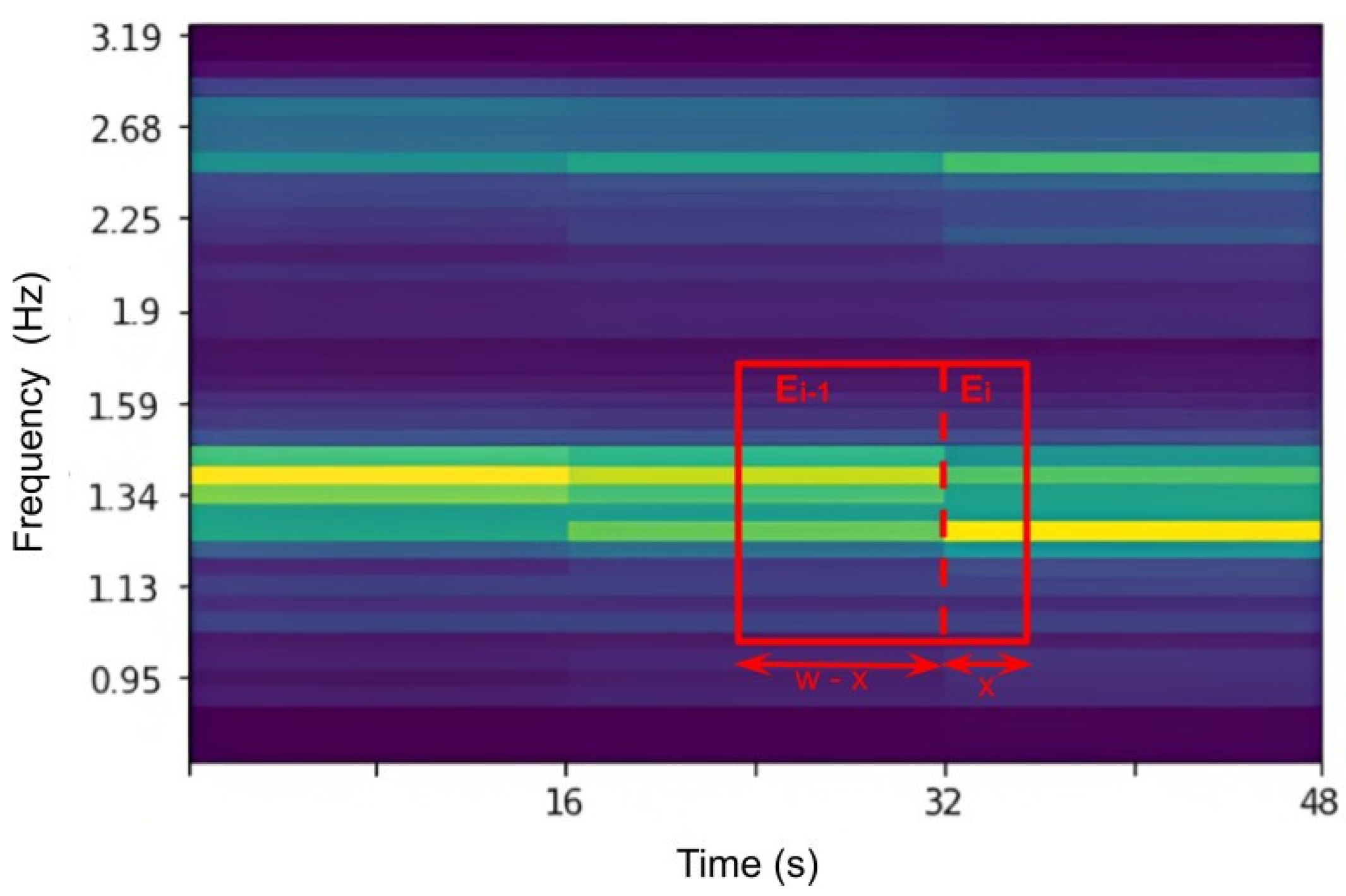
Lastly, an example of coefficients of first-order ST of a PPG signal with a pooling size of 16 s and filter bank of 20 is given in
Figure 2. Frequencies in the y-axis increase exponentially, while time in the x-axis is given as discreet numbers that are multiples of 16 s due to chosen pooling size.
2.2. Windowing
The interpolated rPPG signal is first cleaned with Butterworth bandpass filtering of order 7 with band size 0.7–5 Hz to acquire
rPPGclean. Then, the first-order scattering transform is applied to the obtained signal as explained in
Section 2.1 with a pooling size of 16 s and filter bank of 20. The selection of the pooling size and number of wavelets within the filter bank is task dependent. In the context of our study, simulations revealed that higher frequency resolution generated more favorable outcomes than time resolution. Consequently, a pooling size of 16 s was deemed optimal as it represented a balance between time and frequency resolution. Furthermore, an augmented number of wavelets in the filter bank correlates with an increased frequency resolution. However, this may pose two challenges: firstly, higher computational costs, and secondly, increasing the number of wavelets in the filter bank usually enhances resolution in the higher frequency ranges that are beyond the heart rate region.
Afterward, a windowing step, shown in
Figure 3, is applied on
rPPGclean in the following manner:
1. For each window of size
w calculate the energy around the first harmonic by the given equation:
where
w is window size,
Ei is the energy at time,
i, and
x is the difference between right end of the window and time
i.
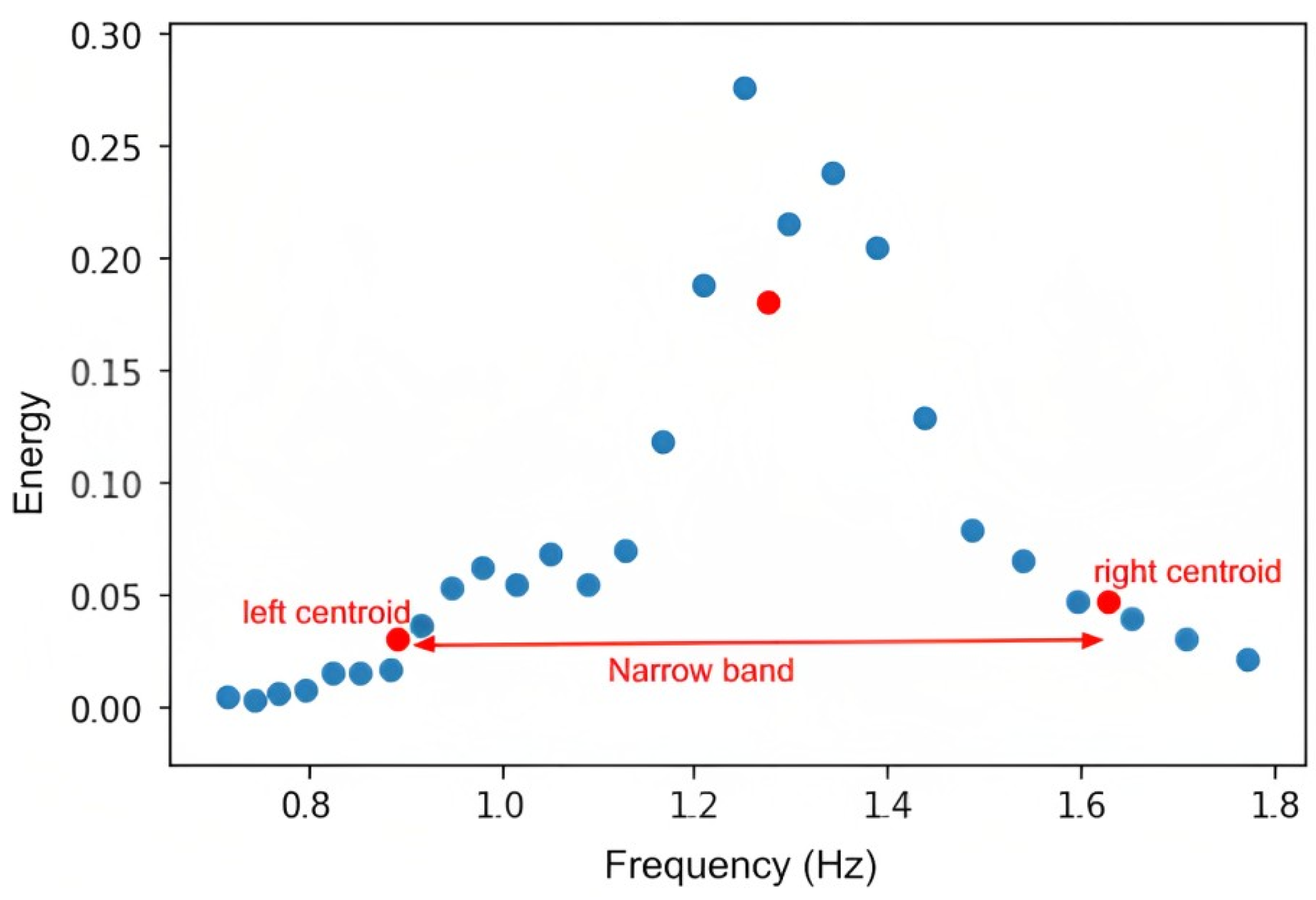
2. Construct K-Means (K = 3) clustering with frequency and energy,
E, as an input and k-mean++ as a centroid initialization to obtain a narrow band, as shown in
Figure 4. The centers of the clusters are shown in red in the
Figure 4. Then, the band size is [left centroid, right centroid].
3. Apply Butterworth bandpass filtering on the windowing signal with previously obtained bands.
4. Subtract the mean of the windowing signal from the windowing signal itself to retain only the pulsatile part and remove the diffuse part.
5. Slide window over whole signal with window size =
w and step size =
s, which can be optimized for different datasets. For instance, in
Figure 3,
w = 14.5 s and
s = 2 s.
6. Reconstruct the cleaned rPPG signal from the windowing segments by adding the segments.
Due to sliding windows, peaks on the edges will be smaller than the rest of the signal. This may result in peak detection issues that can be solved by multiplying both edges of the signal with coefficients (
c), as shown in the pseudo-code (Algorithm 1) below:
| Algorithm 1: peak amplification of the two ends of the signal |
| w ← windowsize |
| s ← stepsize |
| j ← 0 |
| R ← signal |
| whilej≤w/s do |
| c ←
|
| R[ : ] ← R[ : ] |
| j ← j + 1 |
| end while |
2.3. IBI Analysis
Peaks of the reconstructed signal are detected with the automatic multiscale-based peak detection (AMPD) [
19] algorithm and inter-beat-intervals (IBIs) are calculated. Then, refined IBIs are calculated by removing physically impossible regions or misplaced peaks and retaining only those IBIs that satisfy the criteria below:
∀IBI ∈ [400 ms, 1300 ms] **
∀IBI ∈ mean(IBI) ± 0.4mean(IBI)
Non-overlapping window is slid over IBIs with window size 10. IBIs in each window should satisfy ∀IBIwindow ∈ mean(IBIwindow) ± 0.2mean(IBIwindow).
** The boundaries for the IBIs should be chosen based on the task. In this research, we estimate the HRV of adults in a seated position.
6. Discussion
It has been revealed that both the MAE and SD of VIPL-HR and MAHNOB-HCI datasets have significantly dropped after the implementation of the data preprocessing step mentioned in
Section 4. The primary reason for this phenomenon is caused by disconnected or poorly connected electrodes and pulse oximeters, slight motion of fingers inside pulse oximeters, and motion during data collection.
Furthermore, from
Table 4, we note that WaveHRV has lower MAEs on UBFC rPPG and Stroop datasets than on challenging datasets like VIPL-HR and MAHNOB-HCI. UBFC rPPG and Stroop are not compressed and have uniform ambient light, whereas VIPL-HR and MAHNOB-HCI are compressed and recorded under non-uniform or dim lighting. Moreover, in some scenarios of the VIPL-HR, subjects perform large head movements, talk, or are sited further away from the camera.
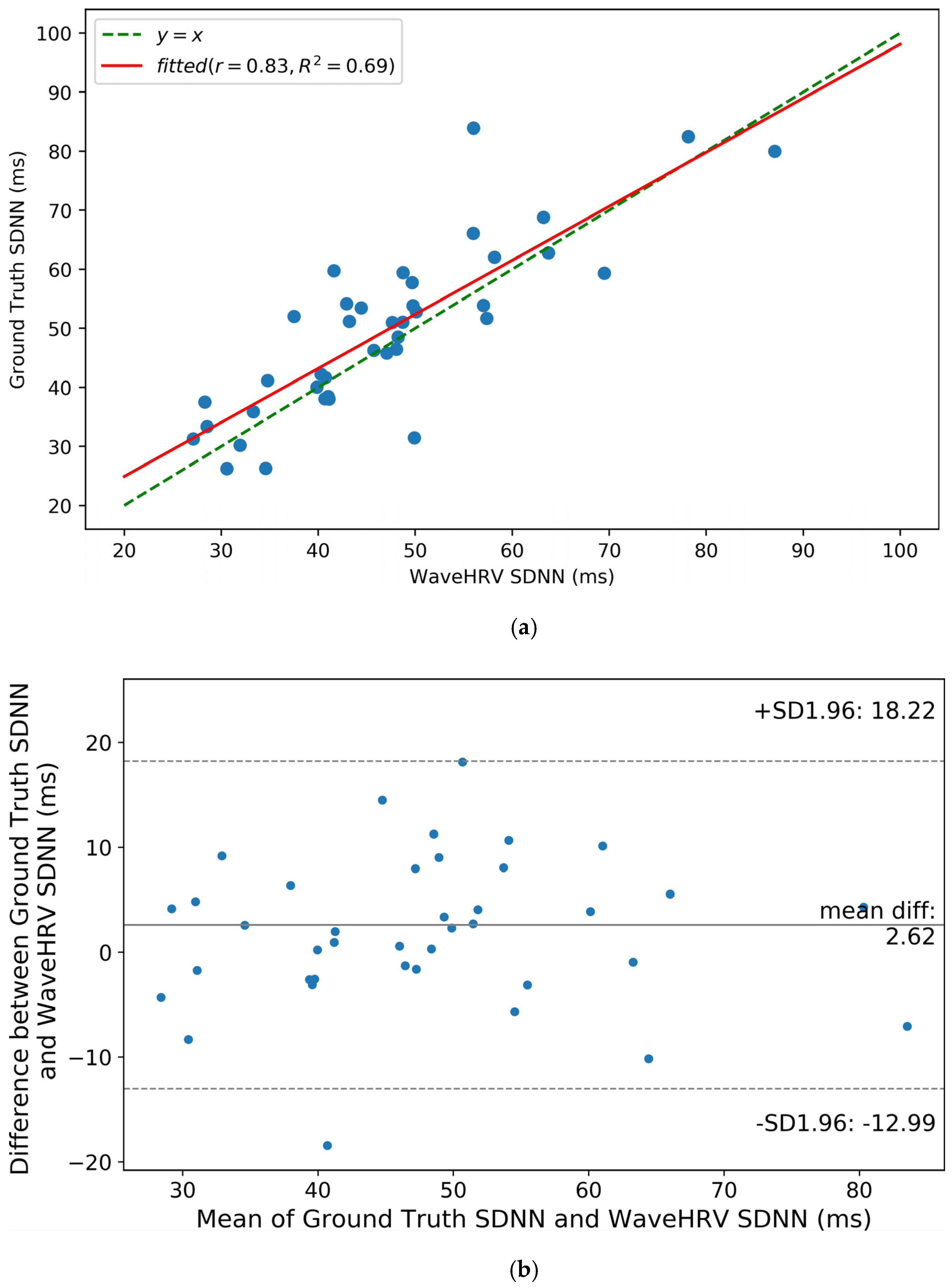
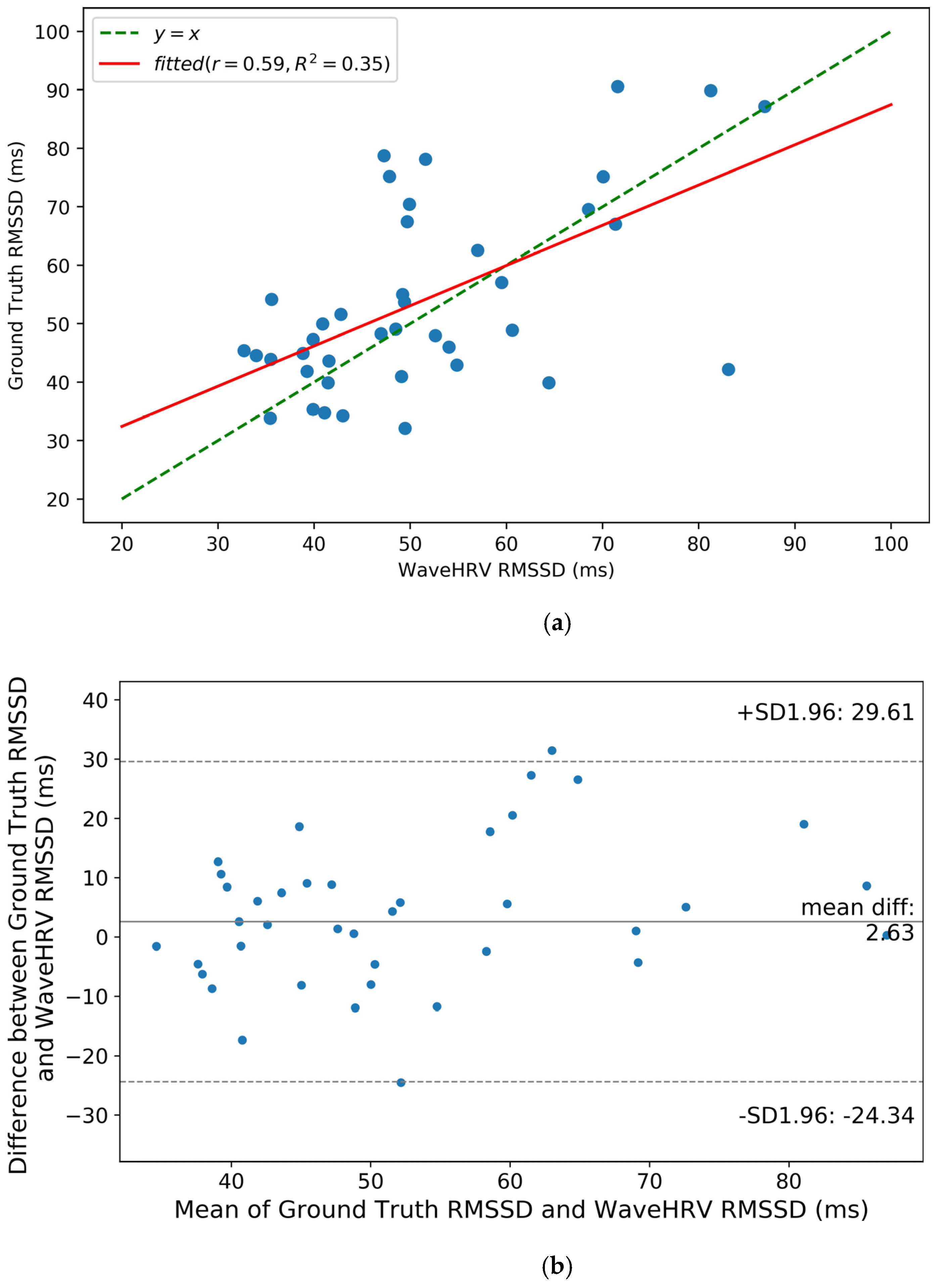
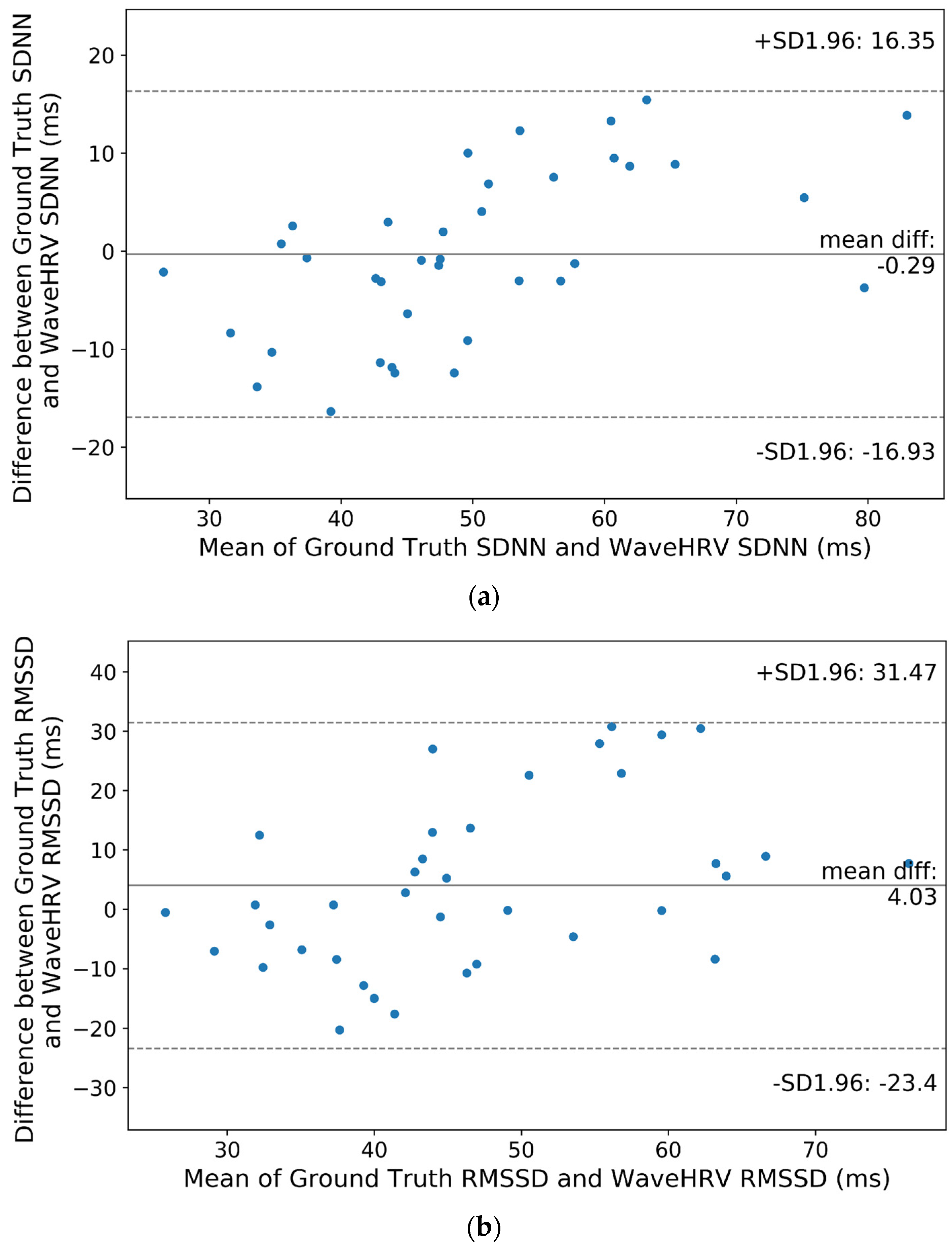
Similar conclusions can be attained from statistical analyses and Bland-Altman plots: when the subjects are not under frequent motion and in a well-lit environment like UBFC rPPG and Stroop datasets, the average WaveHRV SDNN and RMSSD are similar to ground truth SDNN and RMSSD. However, for more challenging, real-life scenarios where there is significant motion and poor lighting conditions like VIPL-HR and MAHNOB-HCI, mean WaveHRV results are different from mean ground truth results.


 ,
, 


