
The Application of Deep Learning to Accurately Identify the Dimensions of Spinal Canal and Intervertebral Foramen as Evaluated by the IoU Index


Abstract

1. Introduction
2. Methods and Materials
2.1. Methods
2.1.1. ResNet
2.1.2. VGG
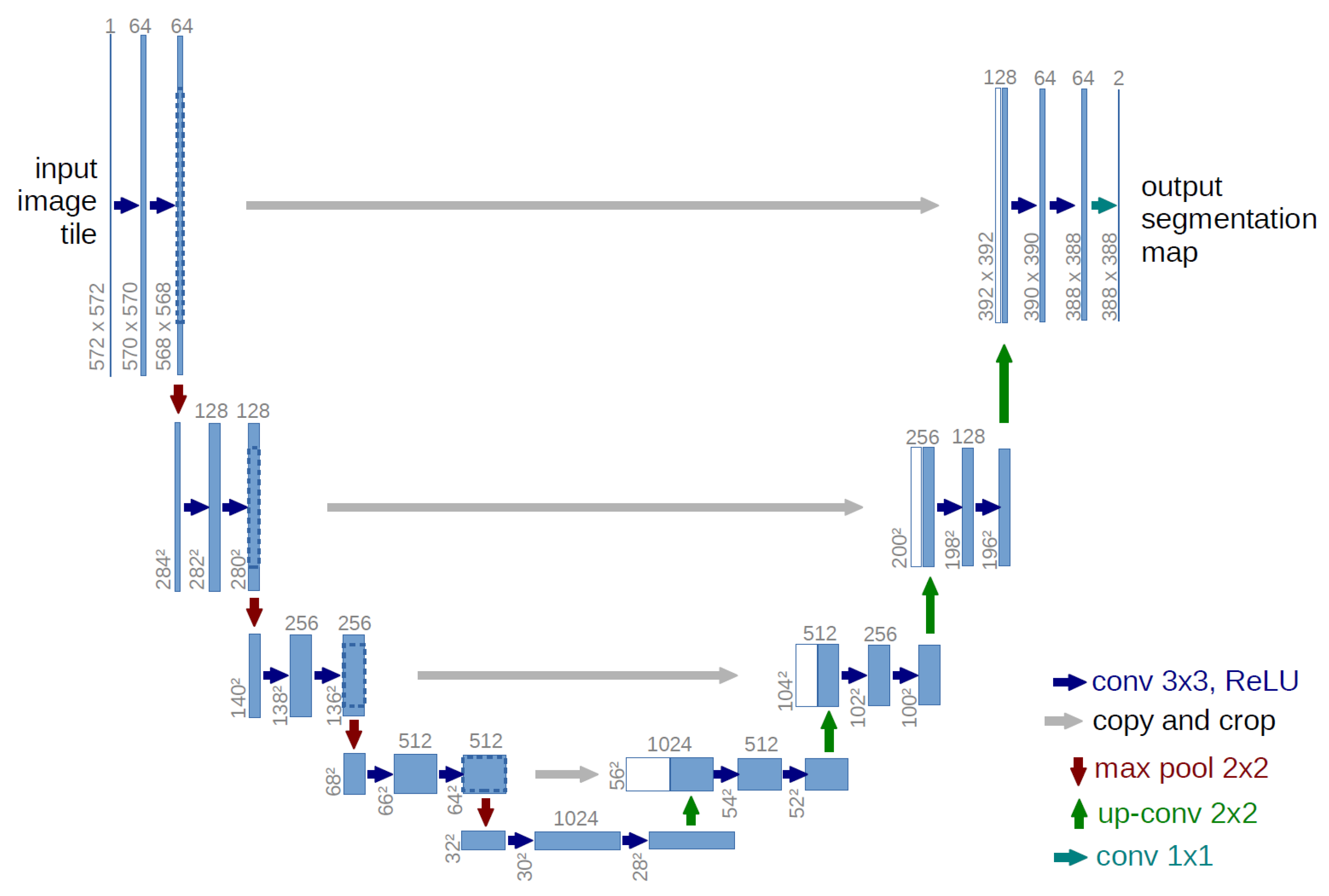
2.1.3. U-Net
2.1.4. YOLO
2.2. Material
2.2.1. Spinal Canal Dataset
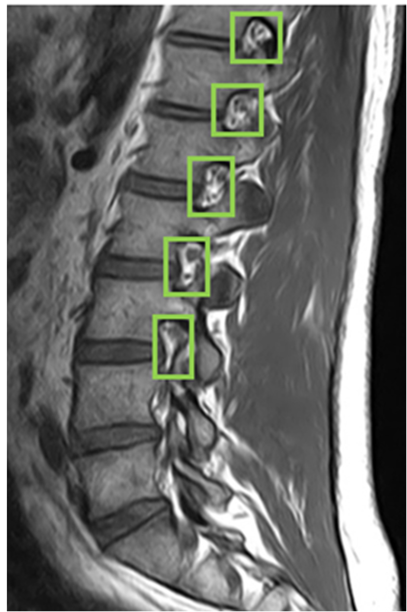
2.2.2. Intervertebral Foramen Dataset
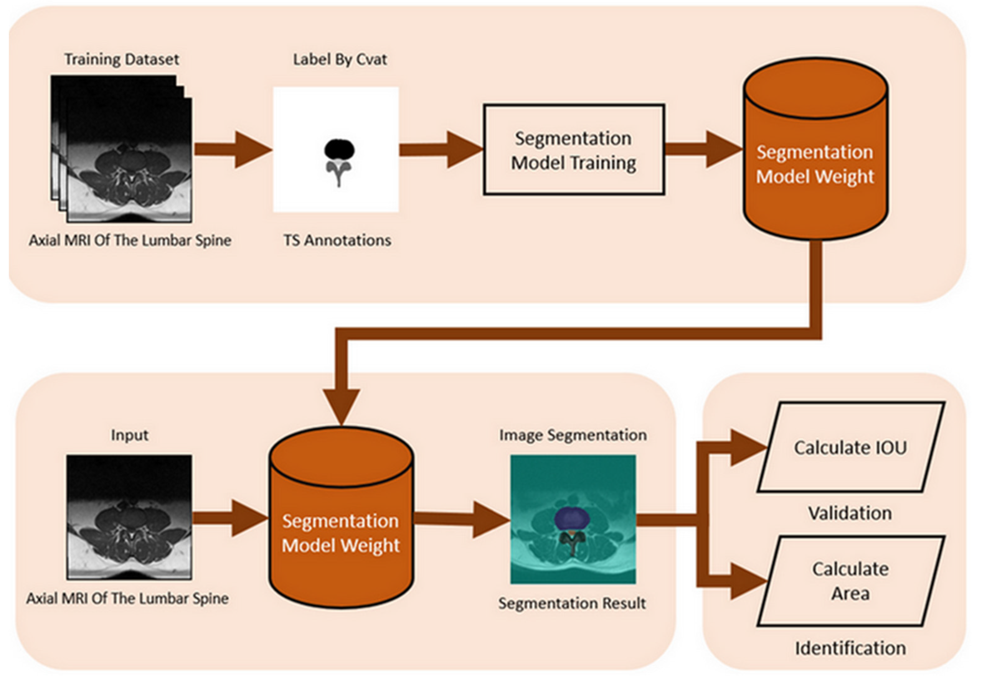
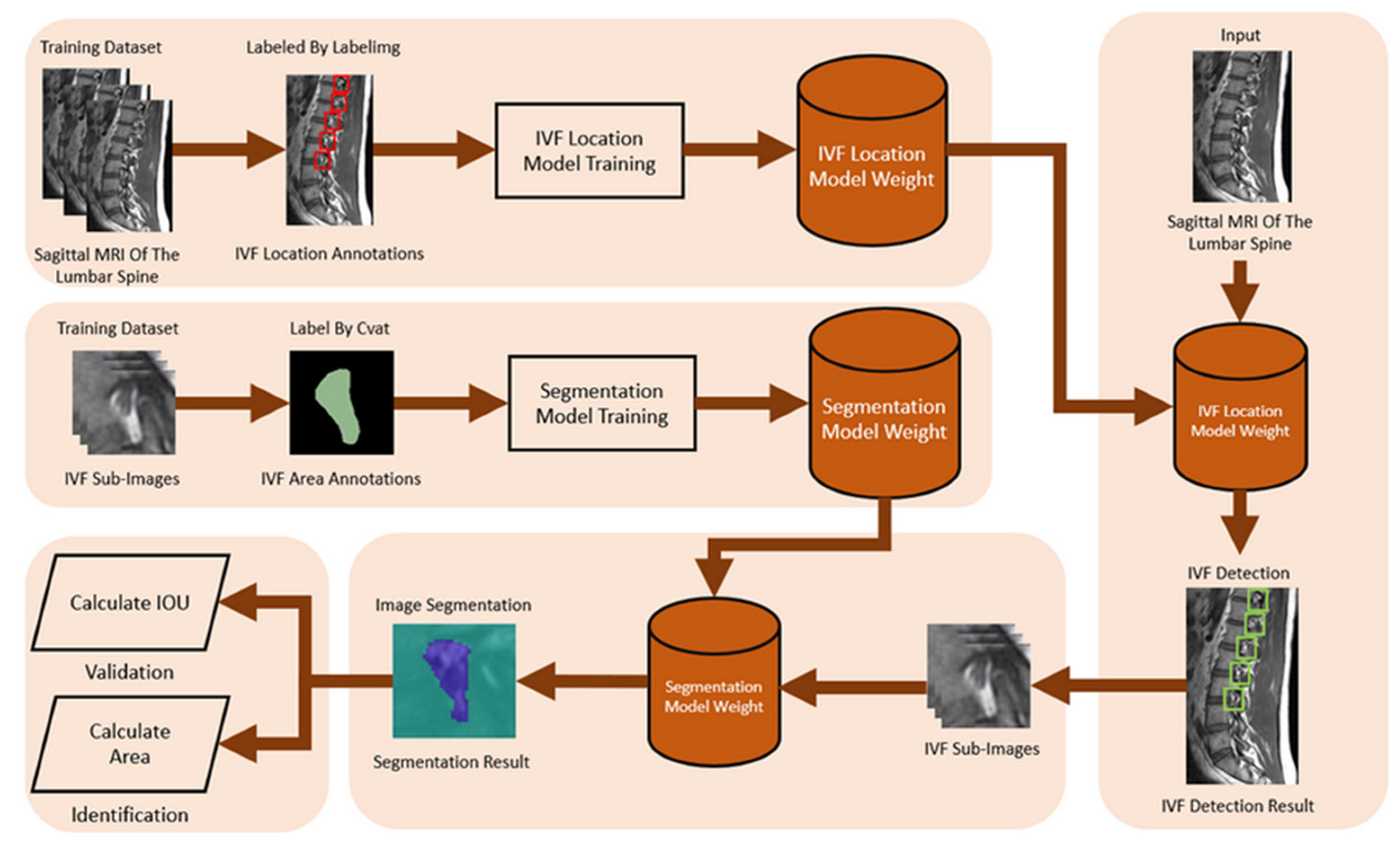
2.2.3. Intervertebral Foramen and Spinal Canal Flowchart
3. Experimental and Hyperparameter Settings
3.1. Experimental
3.2. HyperParameter Settings
3.3. Evaluation Metrics
4. Results
4.1. Spinal Canal Identification
Training Different Segmentation Models Based on Image Category
4.2. Model Comparison
4.3. Intervertebral Foramen Identification
4.4. Assessment of Models and Morphological Processing Techniques
5. Discussion
6. Conclusions
Author Contributions
Funding
Institutional Review Board Statement
Informed Consent Statement
Data Availability Statement
Acknowledgments
Conflicts of Interest
References
- Frost, B.A.; Camarero-Espinosa, S.; Foster, E.J. Materials for the spine: Anatomy, problems, and solutions. Materials 2019, 12, 253. [Google Scholar] [CrossRef]
- Ravindra, V.M.; Senglaub, S.S.; Rattani, A.; Dewan, M.C.; Härtl, R.; Bisson, E.; Park, K.B.; Shrime, M.G. Degenerative lumbar spine disease: Estimating global incidence and worldwide volume. Glob. Spine J. 2018, 8, 784–794. [Google Scholar] [CrossRef] [PubMed]
- Kos, N.; Gradisnik, L.; Velnar, T. A brief review of the degenerative intervertebral disc disease. Med. Arch. 2019, 73, 421. [Google Scholar] [CrossRef]
- Boden, S.D.; Davis, D.; Dina, T.; Patronas, N.; Wiesel, S. Abnormal magnetic-resonance scans of the lumbar spine in asymptomatic subjects. A prospective investigation. J. Bone Jt. Surg. 1990, 72, 403–408. [Google Scholar] [CrossRef]
- Kaul, V.; Enslin, S.; Gross, S.A. History of artificial intelligence in medicine. Gastrointest. Endosc. 2020, 92, 807–812. [Google Scholar] [CrossRef] [PubMed]
- Kulkarni, S.; Seneviratne, N.; Baig, M.S.; Khan, A.H.A. Artificial intelligence in medicine: Where are we now? Acad. Radiol. 2020, 27, 62–70. [Google Scholar] [CrossRef] [PubMed]
- Liu, P.-R.; Lu, L.; Zhang, J.-Y.; Huo, T.-T.; Liu, S.-X.; Ye, Z.-W. Application of artificial intelligence in medicine: An overview. Curr. Med. Sci. 2021, 41, 1105–1115. [Google Scholar] [CrossRef] [PubMed]
- Azimi, P.; Yazdanian, T.; Benzel, E.C.; Aghaei, H.N.; Azhari, S.; Sadeghi, S.; Montazeri, A. A review on the use of artificial intelligence in spinal diseases. Asian Spine J. 2020, 14, 543. [Google Scholar] [CrossRef] [PubMed]
- Hallinan, J.T.P.D.; Zhu, L.; Yang, K.; Makmur, A.; Algazwi, D.A.R.; Thian, Y.L.; Lau, S.; Choo, Y.S.; Eide, S.E.; Yap, Q.V.; et al. Deep learning model for automated detection and classification of central canal, lateral recess, and neural foraminal stenosis at lumbar spine MRI. Radiology 2021, 300, 130–138. [Google Scholar] [CrossRef] [PubMed]
- Lewandrowski, K.-U.; Muraleedharan, N.; Eddy, S.A.; Sobti, V.; Reece, B.D.; León, J.F.R.; Shah, S. Artificial intelligence comparison of the radiologist report with endoscopic predictors of successful transforaminal decompression for painful conditions of the lumber spine: Application of deep learning algorithm interpretation of routine lumbar magnetic resonance imaging scan. Int. J. Spine Surg. 2020, 14 (Suppl. S3), S75–S85. [Google Scholar] [PubMed]
- Rak, M.; Tönnies, K.D. On computerized methods for spine analysis in MRI: A systematic review. Int. J. Comput. Assist. Radiol. Surg. 2016, 11, 1445–1465. [Google Scholar] [CrossRef]
- Dongare, A.; Kharde, R.; Kachare, A.D. Introduction to artificial neural network. Int. J. Eng. Innov. Technol. (IJEIT) 2012, 2, 189–194. [Google Scholar]
- He, K.; Zhang, X.; Ren, S.; Sun, J. Deep residual learning for image recognition. In Proceedings of the IEEE Conference on Computer Vision and Pattern Recognition, Las Vegas, NV, USA, 27–30 June 2016; pp. 770–778. [Google Scholar]
- Simonyan, K.; Zisserman, A. Very deep convolutional networks for large-scale image recognition. arXiv 2014, arXiv:1409.1556. [Google Scholar]
- Krizhevsky, A.; Sutskever, I.; Hinton, G.E. Imagenet classification with deep convolutional neural networks. Adv. Neural Inf. Process. Syst. 2012, 60, 84–90. [Google Scholar] [CrossRef]
- Szegedy, C.; Liu, W.; Jia, Y.; Sermanet, P.; Reed, S.; Anguelov, D.; Erhan, D.; Vanhoucke, V.; Rabinovich, A. Going deeper with convolutions. In Proceedings of the IEEE Conference on Computer Vision and Pattern Recognition, Boston, MA, USA, 7–12 June 2015; pp. 1–9. [Google Scholar]
- Ronneberger, O.; Fischer, P.; Brox, T. U-net: Convolutional networks for biomedical image segmentation. In Medical Image Computing and Computer-Assisted Intervention–MICCAI 2015, Proceedings of the 18th International Conference, Munich, Germany, 5–9 October 2015; Navab, N., Hornegger, J., Wells, W.M., Frangi, A.F., Eds.; Springer: Cham, Switzerland; pp. 234–241.
- Bank, D.; Koenigstein, N.; Giryes, R. Autoencoders. In Machine Learning for Data Science Handbook: Data Mining and Knowledge Discovery Handbook; Rokach, L., Maimon, O., Shmueli, E., Eds.; Springer: Cham, Switzerland, 2023; pp. 353–374. [Google Scholar]
- Bochkovskiy, A.; Wang, C.-Y.; Liao, H.-Y.M. Yolov4: Optimal speed and accuracy of object detection. arXiv 2020, arXiv:2004.10934. [Google Scholar]
- Natalia, F.; Meidia, H.; Afriliana, N.; Al-Kafri, A.S.; Sudirman, S.; Simpson, A.; Sophian, A.; Al-Jumaily, M.; Al-Rashdan, W.; Bashtawi, M. Development of ground truth data for automatic lumbar spine MRI image segmentation. In Proceedings of the 2018 IEEE 20th International Conference on High Performance Computing and Communications; IEEE 16th International Conference on Smart City; IEEE 4th International Conference on Data Science and Systems (HPCC/SmartCity/DSS), Exeter, UK, 28–30 June 2018; pp. 1449–1454. [Google Scholar]
- Al-Kafri, A.S.; Sudirman, S.; Hussain, A.; Al-Jumeily, D.; Natalia, F.; Meidia, H.; Afriliana, N.; Al-Rashdan, W. Boundary delineation of MRI images for lumbar spinal stenosis detection through semantic segmentation using deep neural networks. IEEE Access 2019, 7, 43487–43501. [Google Scholar] [CrossRef]
- Bickle, I. Normal Lumbar Spine MRI. Case Study, Radiopaedia.org. Available online: https://radiopaedia.org/cases/47857 (accessed on 7 September 2016).
- Muzio, B.D. Normal Lumbar Spine MRI—Low-Field MRI Scanner. Case Study, Radiopaedia.org. Available online: https://radiopaedia.org/cases/40976 (accessed on 10 November 2015).
- Hummel, R.A.; Kimia, B.; Zucker, S.W. Deblurring gaussian blur. Comput. Vis. Graph. Image Process. 1987, 38, 66–80. [Google Scholar] [CrossRef]
- Badrinarayanan, V.; Kendall, A.; Cipolla, R. Segnet: A deep convolutional encoder-decoder architecture for image segmentation. IEEE Trans. Pattern Anal. Mach. Intell. 2017, 39, 2481–2495. [Google Scholar] [CrossRef] [PubMed]


| Experimental Environment | Specifications |
|---|---|
| Operating System | Windows 10 |
| CPU | AMD Ryzen 7 2700X Eight-Core Processor 3.70 GHz |
| GPU | GeForce RTX 2070 WINDFORCE 8G |
| CUDA Version | 10.2 |
| RAM | 32.0 GB |
| Framework | Darknet |
| Python | 3.8 |
| Hyperparameter Name | Value |
|---|---|
| learning rate | 0.00261 |
| policy | steps |
| max_batches | 8000 |
| activation | leaky |
| momentum | 0.9 |
| decay | 0.0005 |
| angle | 180 |
| saturation | 1.5 |
| exposure | 1.5 |
| hue | 0.1 |
| gaussian noise | 20 |
| S.No | Encode Model | Decode Model | IoU Mean | IoU Std |
|---|---|---|---|---|
| 1 | VGG16 | U-net | 73.94 | 9.54 |
| 2 | VGG16 | Segnet | 66.94 | 10.38 |
| 3 | Resnet50 | U-net | 77.4 | 8.77 |
| 4 | Resnet50 | Segnet | 68.61 | 12.58 |
| S.No | Encode Model | Decode Model | IoU Mean | IoU Std |
|---|---|---|---|---|
| 1 | VGG16 | U-Net | 61.19 | 10.85 |
| 2 | VGG16 | Segnet | 48.11 | 12.28 |
| 3 | Resnet50 | U-Net | 79.11 | 9.40 |
| 4 | Resnet50 | Segnet | 50.47 | 14.42 |
| S.No | Encode Model | Decode Model | IoU Mean | IoU Std |
|---|---|---|---|---|
| 1 | VGG16 | U-Net | 64.97 | 10.85 |
| 2 | VGG16 | Segnet | 45.26 | 8.99 |
| 3 | Resnet50 | U-Net | 80.89 | 9.44 |
| 4 | Resnet50 | Segnet | 43.09 | 10.60 |
Disclaimer/Publisher’s Note: The statements, opinions and data contained in all publications are solely those of the individual author(s) and contributor(s) and not of MDPI and/or the editor(s). MDPI and/or the editor(s) disclaim responsibility for any injury to people or property resulting from any ideas, methods, instructions or products referred to in the content. |
© 2024 by the authors. Licensee MDPI, Basel, Switzerland. This article is an open access article distributed under the terms and conditions of the Creative Commons Attribution (CC BY) license (https://creativecommons.org/licenses/by/4.0/).
Share and Cite
Wu, C.-Y.; Yeh, W.-C.; Chang, S.-M.; Hsu, C.-W.; Lin, Z.-J. The Application of Deep Learning to Accurately Identify the Dimensions of Spinal Canal and Intervertebral Foramen as Evaluated by the IoU Index. Bioengineering 2024, 11, 981. https://doi.org/10.3390/bioengineering11100981
Wu C-Y, Yeh W-C, Chang S-M, Hsu C-W, Lin Z-J. The Application of Deep Learning to Accurately Identify the Dimensions of Spinal Canal and Intervertebral Foramen as Evaluated by the IoU Index. Bioengineering. 2024; 11(10):981. https://doi.org/10.3390/bioengineering11100981
Chicago/Turabian StyleWu, Chih-Ying, Wei-Chang Yeh, Shiaw-Meng Chang, Che-Wei Hsu, and Zi-Jie Lin. 2024. "The Application of Deep Learning to Accurately Identify the Dimensions of Spinal Canal and Intervertebral Foramen as Evaluated by the IoU Index" Bioengineering 11, no. 10: 981. https://doi.org/10.3390/bioengineering11100981
APA StyleWu, C.-Y., Yeh, W.-C., Chang, S.-M., Hsu, C.-W., & Lin, Z.-J. (2024). The Application of Deep Learning to Accurately Identify the Dimensions of Spinal Canal and Intervertebral Foramen as Evaluated by the IoU Index. Bioengineering, 11(10), 981. https://doi.org/10.3390/bioengineering11100981