
Computational Modeling Approach to Profile Hemodynamical Behavior in a Healthy Aorta

 ,
,  , ,
, ,  , and
, and 
Abstract

1. Introduction
2. Materials and Methods
2.1. Aortic Geometry and Boundary Conditions
2.2. CFD Setup
2.3. Wall Shear Stress Parameters
2.4. Mesh Generation and Sensitivity
3. Results
3.1. Validation of the Study
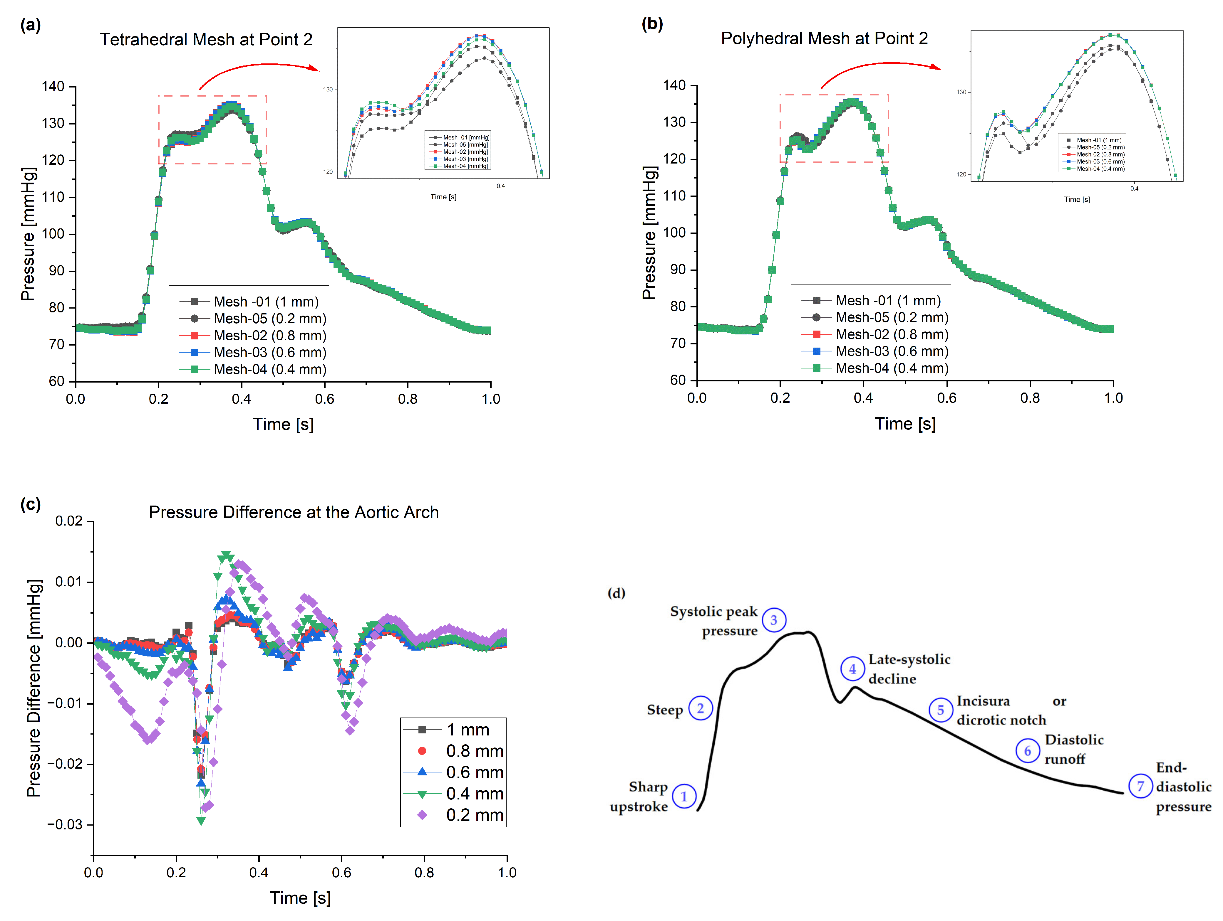
3.2. Pressure Waveform
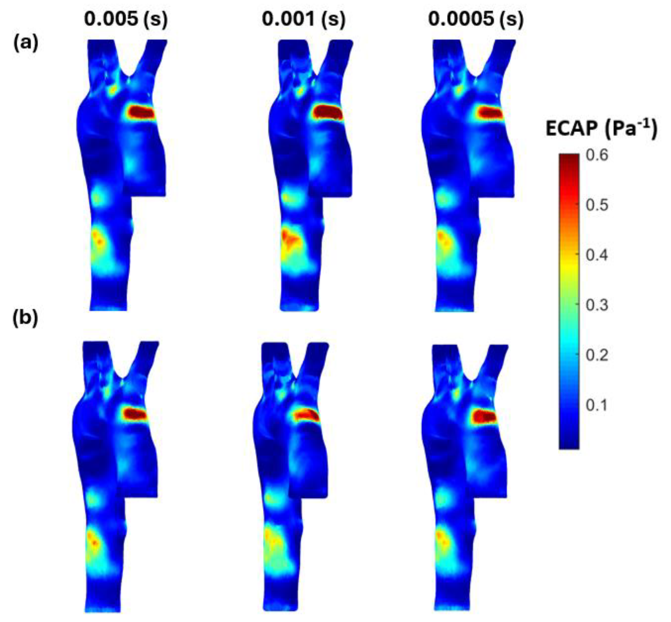
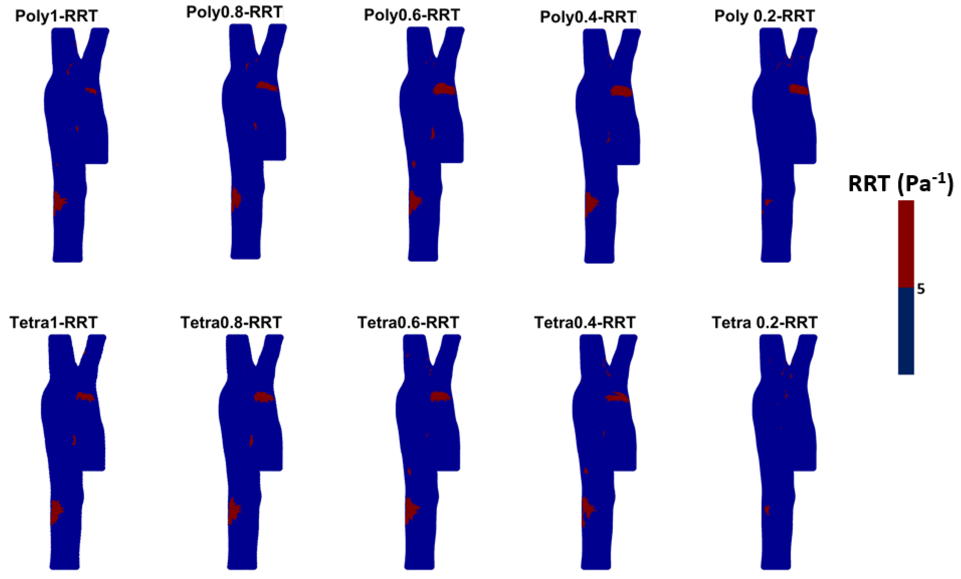
3.3. Endothelial Cell Characteristics
4. Discussion
- Both tetrahedral and polyhedral meshes at a 0.2 mm element size provided high accuracy, with validation against clinical data showing an average error of 3.3% for polyhedral and 3.1% for tetrahedral meshes. Notably, the polyhedral mesh achieved a 54% reduction in simulation time (103 min) compared to the tetrahedral mesh (222 min) while maintaining comparable results;
- The pressure waveform analysis indicated minimal differences between mesh types and sizes. A 0.4 mm polyhedral mesh was found to be a practical balance, producing accurate waveforms in just 37 min;
- WSS-based parameters (TAWSS, OSI, RRT, and ECAP) revealed similar trends across both mesh types, though finer meshes captured more detailed variations. The polyhedral mesh demonstrated better gradient handling, making it suitable for simulating complex vascular regions like the aortic arch.
Limitations and Further Study
5. Conclusions
Author Contributions
Funding
Institutional Review Board Statement
Informed Consent Statement
Data Availability Statement
Acknowledgments
Conflicts of Interest
Appendix A


Appendix B


References
- Martin, S.S.; Aday, A.W.; Almarzooq, Z.I.; Anderson, C.A.; Arora, P.; Avery, C.L.; Baker-Smith, C.M.; Gibbs, B.B.; Beaton, A.Z.; Boehme, A.K.; et al. 2024 Heart Disease and Stroke Statistics: A Report of US and Global Data From the American Heart Association. Circulation 2024, 149, e347–e913. [Google Scholar] [CrossRef] [PubMed]
- AL-Rawi, M.; AL-Jumaily, A.M.; Belkacemi, D. Non-invasive diagnostics of blockage growth in the descending aorta-computational approach. Med. Biol. Eng. comput. 2022, 60, 3265–3279. [Google Scholar] [CrossRef] [PubMed]
- Conrad, N.; Molenberghs, G.; Verbeke, G.; Zaccardi, F.; Lawson, C.; Friday, J.M.; Su, H.; Jhund, P.S.; Sattar, N.; Rahimi, K.; et al. Trends in cardiovascular disease incidence among 22 million people in the UK over 20 years: Population-based study. BMJ 2024, 385, e078523. [Google Scholar] [CrossRef] [PubMed]
- Timmis, A.; Vardas, P.; Townsend, N.; Torbica, A.; Katus, H.; de Smedt, D.; Gale, C.P.; Maggioni, A.P.; Petersen, S.E.; Huculeci, R.; et al. European Society of Cardiology. European Society of Cardiology: Cardiovascular disease statistics 2021. Eur. Heart J. 2022, 43, 716–799. [Google Scholar] [CrossRef] [PubMed]
- Andersson, C.; Vasan, R.S. Epidemiology of cardiovascular disease in young individuals. Nat. Rev. Cardiol. 2018, 15, 230–240. [Google Scholar] [CrossRef]
- Abdalla, S.M.; Yu, S.; Galea, S. Trends in Cardiovascular Disease Prevalence by Income Level in the United States. JAMA Netw. Open 2020, 3, e2018150. [Google Scholar] [CrossRef]
- Roth, G.A.; Mensah, G.A.; Johnson, C.O.; Addolorato, G.; Ammirati, E.; Baddour, L.M.; Barengo, N.C.; Beaton, A.Z.; Benjamin, E.J.; Benziger, C.P.; et al. GBD-NHLBI-JACC Global Burden of Cardiovascular Diseases Writing Group. Global Burden of Cardiovascular Diseases and Risk Factors, 1990–2019: Update From the GBD 2019 Study. J. Am. Coll. Cardiol. 2020, 76, 2982–3021. [Google Scholar] [CrossRef]
- National Center for Health Statistics. Multiple Cause of Death 2018–2021 on CDC WONDER Database. Available online: https://wonder.cdc.gov/mcd.html (accessed on 14 November 2023).
- Tsao, C.W.; Aday, A.W.; Almarzooq, Z.I.; Anderson, C.A.; Arora, P.; Avery, C.L.; Baker-Smith, C.M.; Beaton, A.Z.; Boehme, A.K.; Buxton, A.E.; et al. Heart Disease and Stroke Statistics—2023 Update: A Report From the American Heart Association. Circulation 2023, 147, E93–E621. [Google Scholar] [CrossRef]
- Healthdirect Australia. Heart Foundation. Health Direct. Available online: https://www.healthdirect.gov.au/partners/heart-foundation (accessed on 14 November 2023).
- Heart Foundation, New Zealand. Latest Heart Disease Statistics. Available online: https://www.heartfoundation.org.nz/statistics (accessed on 14 November 2023).
- Al-Rawi, M.; Al-Jumaily, A.M. Assessing abdominal aorta narrowing using computational fluid dynamics. Med. Biol. Eng. Comput. 2016, 54, 843–853. [Google Scholar] [CrossRef]
- Zhu, Y. Clinical validation and assessment of aortic hemodynamics using computational fluid dynamics simulations from computed tomography angiography. BioMed. Eng. Online 2018, 17, 53. [Google Scholar] [CrossRef]
- Numata, S.; Itatani, K.; Kanda, K.; Doi, K.; Yamazaki, S.; Morimoto, K.; Manabe, K.; Ikemoto, K.; Yaku, H. Blood flow analysis of the aortic arch using computational fluid dynamics. Eur. J. Cardio-Thorac. Surg. 2016, 49, 1578–1585. [Google Scholar] [CrossRef] [PubMed]
- Al-Rawi, M.; Al-Jumaily, A.; Belkacemi, D. Do Long Aorta Branches Impact on the Rheological Properties? In Proceedings of the ASME 2021 International Mechanical Engineering Congress and Exposition, Virtual, Online, 1–5 November 2021; Volume 5: Biomedical and Biotechnology. ASME: New York, NY, USA, 2022; p. V005T05A032. [Google Scholar] [CrossRef]
- Kamrath, B.D.; Suess, T.N.; Gent, S.P. Assessment of Pulsatile Blood Flow Models for the Descending Aorta Using CFD. In Proceedings of the ASME 2015 International Mechanical Engineering Congress and Exposition, Houston, TX, USA, 13–19 November 2015; Volume 3: Biomedical and Biotechnology Engineering. ASME: New York, NY, USA, 2016; p. V003T03A100. [Google Scholar] [CrossRef]
- Gao, F.; Ohta, O.; Matsuzawa, T. Fluid-structure interaction in layered aortic arch aneurysm model: Assessing the combined influence of arch aneurysm and wall stiffness. Australas. Phys. Eng. Sci. Med. 2008, 31, 32–41. [Google Scholar] [CrossRef] [PubMed]
- Algabri, Y.A.; Rookkapan, S.; Gramigna, V.; Espino, D.M.; Chatpun, S. Computational study on hemodynamic changes in patient-specific proximal neck angulation of abdominal aortic aneurysm with time-varying velocity. Australas. Phys. Eng. Sci. Med. 2019, 42, 181–190. [Google Scholar] [CrossRef] [PubMed]
- Alkhatib, F.; Wittek, A.; Zwick, B.F.; Bourantas, G.C.; Miller, K. Computation for biomechanical analysis of aortic aneurysms: The importance of computational grid. Comput. Methods Biomech. Biomed. Eng. 2023, 27, 994–1010. [Google Scholar] [CrossRef] [PubMed]
- Takizawa, K.; Tezduyar, T.E.; Uchikawa, H.; Terahara, T.; Sasaki, T.; Yoshida, A. Mesh refinement influence and cardiac-cycle flow periodicity in aorta flow analysis with isogeometric discretization. Comput. Fluids 2019, 179, 790–798. [Google Scholar] [CrossRef]
- Zhu, C.; Seo, J.; Mittal, R. Computational modelling and analysis of haemodynamics in a simple model of aortic stenosis. J. Fluid. Mech. 2018, 851, 23–49. [Google Scholar] [CrossRef]
- Trenti, C.; Ziegler, M.; Bjarnegã¥Rd, N.; Ebbers, T.; Lindenberger, M.; Dyverfeldt, P. Wall shear stress and relative residence time as potential risk factors for abdominal aortic aneurysms in males: A 4D flow cardiovascular magnetic resonance case–control study. J. Cardiovasc. Magn. Reason. 2022, 24, 18. [Google Scholar] [CrossRef]
- Tang, X.; Wu, C. A predictive surrogate model for hemodynamics and structural prediction in abdominal aorta for different physiological conditions. Comput. Methods Programs Biomed. 2024, 243, 107931. [Google Scholar] [CrossRef]
- Simão, M.; Ferreira, J.; Tomás, A.C.; Fragata, J.; Ramos, H.M. Aorta Ascending Aneurysm Analysis Using CFD Models towards Possible Anomalies. Fluids 2017, 2, 31. [Google Scholar] [CrossRef]
- Petuchova, A.; Maknickas, A. Computational analysis of aortic haemodynamics in the presence of ascending aortic aneurysm. Technol. Health Care 2021, 30, 187–200. [Google Scholar] [CrossRef]
- Minderhoud, S.C.; Arrouby, A.; Hoven, A.T.v.D.; Bons, L.R.; Chelu, R.G.; Kardys, I.; Rizopoulos, D.; Korteland, S.-A.; Bosch, A.E.v.D.; Budde, R.P.; et al. Regional Aortic Wall Shear Stress Increases over Time in Patients with a Bicuspid Aortic Valve. J. Cardiovasc. Magn. Reson. 2024, 101070. [Google Scholar] [CrossRef] [PubMed]
- Minderhoud, S.C.S.; Roos-Hesselink, J.W.; Chelu, R.G.; Bons, L.R.; Hoven, A.T.v.D.; Korteland, S.-A.; Bosch, A.E.v.D.; Budde, R.P.J.; Wentzel, J.J.; Hirsch, A. Wall shear stress angle is associated with aortic growth in bicuspid aortic valve patients. Eur. Heart J. Cardiovasc. Imaging 2022, 23, 1680–1689. [Google Scholar] [CrossRef] [PubMed]
- Soulat, G.; Scott, M.B.; Allen, B.D.; Avery, R.; Bonow, R.O.; Malaisrie, S.C.; McCarthy, P.; Fedak, P.W.; Barker, A.J.; Markl, M. Association of Regional Wall Shear Stress and Progressive Ascending Aorta Dilation in Bicuspid Aortic Valve. JACC Cardiovasc. Imaging 2022, 15, 33–42. [Google Scholar] [CrossRef]
- Chiu, J.J.; Chien, S. Effects of disturbed flow on vascular endothelium: Pathophysiological basis and clinical perspectives. Physiol. Rev. 2011, 91, 327–387. [Google Scholar] [CrossRef] [PubMed]
- Osswald, A.; Karmonik, C.; Anderson, J.; Rengier, F.; Kretzler, M.; Engelke, J.; Kallenbach, K.; Kotelis, D.; Partovi, S.; Böckler, D. Elevated Wall Shear Stress in Aortic Type B Dissection May Relate to Retrograde Aortic Type A Dissection: A Computational Fluid Dynamics Pilot Study. Eur. J. Cardiothorac. Surg. 2017, 54, 324–330. [Google Scholar] [CrossRef] [PubMed]
- Meng, X.; Wu, J.; Chen, D.; Wang, C.; Wu, Y.; Sun, T.; Chen, J. Ascending aortic volume: A feasible indicator for ascending aortic aneurysm elective surgery? Acta Biomater. 2023, 167, 100–108. [Google Scholar] [CrossRef]
- Qu, W.; Li, X.; Huang, H.; Xie, C.; Song, H. Mechanisms of the ascites volume differences between patients receiving a left or right hemi-liver graft liver transplantation: From biofluidic analysis. Comput. Methods Programs Biomed. 2022, 226, 107196. [Google Scholar] [CrossRef]
- Caballero, A.; Laín, S. A review on Computational fluid dynamics modelling in human thoracic aorta. Cardiovasc. Eng. Tech. 2013, 4, 103–130. [Google Scholar] [CrossRef]
- Kumar, N.; Khader, A.; Pai, R.; Kyriacou, P.; Khan, S.; Koteshwara, P. Computational fluid dynamic study on effect of Carreau-Yasuda and Newtonian blood viscosity models on hemodynamic parameters. J. Comput. Methods Sci. Eng. 2019, 19, 465–477. [Google Scholar] [CrossRef]
- Spiegel, M.; Redel, T.; Zhang, Y.; Struffert, T.; Hornegger, J.; Grossman, R.; Doerfler, A.; Karmonik, C. Tetrahedral and polyhedral mesh evaluation for cerebral hemodynamic simulation-A comparison. In Proceedings of the 2009 Annual International Conference of the IEEE Engineering in Medicine and Biology Society, Minneapolis, MN, USA, 3–6 September 2009; pp. 2787–2790. [Google Scholar] [CrossRef]
- Wellnhofer, E.; Goubergrits, L.; Kertzscher, U.; Affeld, K.; Fleck, E. Novel non-dimensional approach to comparison of wall shear stress distributions in coronary arteries of different groups of patients. Atherosclerosis 2009, 202, 483–490. [Google Scholar] [CrossRef]
- Martelli, F.; Milani, M.; Montorsi, L.; Ligabue, G.; Torricelli, P. Fluid-Structure Interaction of Blood Flow in Human Aorta Under Dynamic Conditions: A Numerical Approach. In Proceedings of the ASME 2018 International Mechanical Engineering Congress and Exposition, Pittsburgh, PE, USA, 9–15 November 2018; Volume 3: Biomedical and Biotechnology Engineering. ASME: New York, NY, USA, 2019; p. V003T04A054. [Google Scholar] [CrossRef]
- Al-Rawi, M.; Belkacemi, D.; Lim, E.T.A.; Khashram, M. Investigation of Type A Aortic Dissection Using Computational Modelling. Biomedicines 2024, 12, 1973. [Google Scholar] [CrossRef]
- Wang, X.; Shen, Y.; Shang, M.; Liu, X.; Munn, L.L. Endothelial mechanobiology in atherosclerosis. Cardiovasc. Res. 2023, 119, 1656–1675. [Google Scholar] [CrossRef]
- Soudah, E.; Ng, E.Y.K.; Loong, T.H.; Bordone, M.; Pua, U.; Narayanan, S. CFD Modelling of Abdominal Aortic Aneurysm on Hemodynamic Loads Using a Realistic Geometry with CT. Comput. Math. Methods Med. 2013, 2013, e472564. [Google Scholar] [CrossRef]
- Karimi, S.; Dabagh, M.; Vasava, P.; Dadvar, M.; Dabir, B.; Jalali, P. Effect of rheological models on the hemodynamics within human aorta: CFD study on CT image-based geometry. J. Non-Newton. Fluid Mech. 2014, 207, 42–52. [Google Scholar] [CrossRef]
- Cilla, M.; Casales, M.; Peña, E.; Martínez, M.Á.; Malvè, M. A parametric model for studying the aorta hemodynamics by means of the computational fluid dynamics. J. Biomech. 2020, 103, 109691. [Google Scholar] [CrossRef] [PubMed]
- He, Y.; Northrup, H.; Le, H.; Cheung, A.K.; Berceli, S.A.; Shiu, Y.T. Medical Image-Based Computational Fluid Dynamics and Fluid-Structure Interaction Analysis in Vascular Diseases. Front. Bioeng. Biotechnol. 2022, 10, 855791. [Google Scholar] [CrossRef] [PubMed]
- Tse, K.M.; Chang, R.S.; Lee, H.P.; Lim, S.P.; Venkatesh, S.K.; Ho, P. A computational fluid dynamics study on geometrical influence of the aorta on haemodynamics. Eur. J. Cardiothorac. Surg. 2012, 43, 829–838. [Google Scholar] [CrossRef]
- Etli, M.; Canbolat, G.; Karahan, O.; Koru, M. Numerical investigation of patient-specific thoracic aortic aneurysms and comparison with normal subject via computational fluid dynamics (CFD). Med. Biol. Eng. Comput. 2020, 59, 71–84. [Google Scholar] [CrossRef] [PubMed]
- Leuprecht, A.; Kozerke, S.; Boesiger, P.; Perktold, K. Blood flow in the human ascending aorta: A combined MRI and CFD study. J. Eng. Math. 2003, 47, 387–404. [Google Scholar] [CrossRef]
- Hashemi, J.; Patel, B.; Chatzizisis, Y.S.; Kassab, G.S. Study of coronary atherosclerosis using blood residence Time. Front. Physiol. 2021, 12, 625420. [Google Scholar] [CrossRef]
- Pirentis, A.P.; Kalogerakos, P.; Mojibian, H.; Elefteriades, J.A.; Lazopoulos, G.; Papaharilaou, Y. Automated ascending aorta delineation from ECG-gated computed tomography images. Med. Biol. Eng. Comput. 2022, 60, 2095–2108. [Google Scholar] [CrossRef] [PubMed]
- Condemi, F.; Campisi, S.; Viallon, M.; Croisille, P.; Fuzelier, J.; Avril, S. Ascending thoracic aorta aneurysm repair induces positive hemodynamic outcomes in a patient with unchanged bicuspid aortic valve. J. Bioeng. 2018, 81, 145–148. [Google Scholar] [CrossRef] [PubMed]
- Bit, A.; Alblawi, A.; Chattopadhyay, H.; Quais, Q.A.; Benim, A.C.; Rahimi-Gorji, M.; Do, H. Three dimensional numerical analysis of hemodynamic of stenosed artery considering realistic outlet boundary conditions. Comput. Methods Programs Biomed. 2020, 185, 105163. [Google Scholar] [CrossRef]
- Belkacemi, D.; Abbés, M.T.; Al-Rawi, M.; Al-Jumaily, A.M.; Bachene, S.; Laribi, B. Intraluminal thrombus characteristics in AAA patients: Non-Invasive diagnosis using CFD. Bioengineering 2023, 10, 540. [Google Scholar] [CrossRef] [PubMed]
- Kelsey, L.J.; Powell, J.T.; Norman, P.E.; Miller, K.; Doyle, B.J. A comparison of hemodynamic metrics and intraluminal thrombus burden in a common iliac artery aneurysm. Int. J. Numer. Methods Biomed. Eng. 2017, 33, e2821. [Google Scholar] [CrossRef]
- Tzirakis, K.; Kamarianakis, Y.; Kontopodis, N.; Ioannou, C.V. The Effect of Blood Rheology and Inlet Boundary Conditions on Realistic Abdominal Aortic Aneurysms under Pulsatile Flow Conditions. Bioengineering 2023, 10, 272. [Google Scholar] [CrossRef]
- Belkacemi, D.; Al-Rawi, M.; Abbes, M.T.; Laribi, B. Flow Behaviour and Wall Shear Stress Derivatives in Abdominal Aortic Aneurysm Models: A Detailed CFD Analysis into Asymmetry Effect. CFD Lett. 2022, 14, 60–74. [Google Scholar] [CrossRef]
- Peiffer, V.; Sherwin, S.J.; Weinberg, P.D. Computation in the rabbit aorta of a new metric–the transverse wall shear stress to quantify the multidirectional character of disturbed blood flow. J. Biomech. 2013, 46, 2651–2658. [Google Scholar] [CrossRef]
- Himburg, H.A.; Grzybowski, D.M.; Hazel, A.L.; LaMack, J.A.; Li, X.M.; Friedman, M.H. Spatial comparison between wall shear stress measures and porcine arterial endothelial permeability. Am. J. Physiol. Heart Circ. 2004, 286, H1916–H1922. [Google Scholar] [CrossRef]
- Morbiducci, U.; Gallo, D.; Ponzini, R.; Massai, D.N.C.; Antiga, L.; Montevecchi, F.M.; Redaelli, A. Quantitative analysis of bulk flow in Image-Based Hemodynamic Models of the carotid bifurcation: The influence of outflow conditions as test case. Ann. Biomed. Eng. 2010, 38, 3688–3705. [Google Scholar] [CrossRef]
- Achille, P.D.; Tellides, G.; Figueroa, C.A.; Humphrey, J.D. A haemodynamic predictor of intraluminal thrombus formation in abdominal aortic aneurysms. Proc. R. Soc. A Math. Phys. Eng. Sci. 2014, 470, 20140163. [Google Scholar] [CrossRef]
- Mutlu, O.; Salman, H.E.; Al-Thani, H.; El-Menyar, A.; Qidwai, U.; Yalcin, H.C. How does hemodynamics affect rupture tissue mechanics in abdominal aortic aneurysm: Focus on wall shear stress derived parameters, time-averaged wall shear stress, oscillatory shear index, endothelial cell activation potential, and relative residence time. Comput. Biol. Med. 2023, 154, 106609. [Google Scholar] [CrossRef] [PubMed]
- Ohhara, Y.; Oshima, M.; Iwai, T.; Kitajima, H.; Yajima, Y.; Mitsudo, K.; Krdy, A.; Tohnai, I. Investigation of blood flow in the external carotid artery and its branches with a new 0D peripheral model. BioMed. Eng. Online 2016, 15, 1. [Google Scholar] [CrossRef] [PubMed]
- Curta, A.; Jaber, A.; Rieber, J.; Hetterich, H. Estimation of endothelial shear stress in atherosclerotic lesions detected by intravascular ultrasound using computational fluid dynamics from coronary CT scans with a pulsatile blood flow and an individualized blood viscosity. Clin. Hemorheol. Microcirc. 2021, 79, 505–518. [Google Scholar] [CrossRef] [PubMed]
- Cheng, H.; Zhong, W.; Wang, L.; Zhang, Q.; Ma, X.; Wang, Y.; Wang, S.; He, C.; Wei, Q.; Fu, C. Effects of shear stress on vascular endothelial functions in atherosclerosis and potential therapeutic approaches. Biomed. Pharmacother. 2023, 158, 114198. [Google Scholar] [CrossRef] [PubMed]
- Fuchs, A.; Berg, N.; Fuchs, L.; Prahl Wittberg, L. Assessment of Rheological Models Applied to Blood Flow in Human Thoracic Aorta. Bioengineering 2023, 10, 1240. [Google Scholar] [CrossRef]
- Tzirakis, K.; Kamarianakis, Y.; Kontopodis, N.; Ioannou, C.V. Classification of Blood Rheological Models through an Idealized Symmetrical Bifurcation. Symmetry 2023, 15, 630. [Google Scholar] [CrossRef]
- Al-Rawi, M.; Djelloul, B.; Al-Jumaily, A. Comparison of Laminar and Turbulent K-Omega Shear Stress Transport Models Under Realistic Boundary Conditions Using Clinical Data for Arterial Stenosis. J. Eng. Sci. Med. Diagn. Ther. 2024. [Google Scholar] [CrossRef]
- Al-Rawi, M. Two-Way Interaction (Aorta Blood-Artery) Using Computational Fluid Dynamics (CFD) Simulation. In Proceedings of the IEEE 4th Eurasia Conference on Biomedical Engineering, Healthcare and Sustainability (ECBIOS), Tainan, Taiwan, 27–29 May 2022; pp. 79–82. [Google Scholar] [CrossRef]


| Location | Diameter (mm) | Area (mm2) | Boundary Condition | Waveform |
|---|---|---|---|---|
| Ascending aorta (AA) | 35.88 | 100.15 | Ascending inlet blood velocity waveform |  |
| Iliac (I) | 29.74 | 65.58 | Iliac outlet blood pressure waveform |  |
| Brachiocephalic (BC) | 13.48 | 14.02 | Outlet blood pressure waveform | 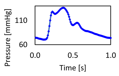 |
| Left common carotid (LCC) | 8.43 | 5.36 | ||
| Left subclavian (LS) | 11.75 | 10.00 |
| (A) | ||||||
| Element Size [mm] | Element Number (T) | Vmax(T) [m/s] | % | WSSmax(T) [Pa] | % | Time (T) (min) |
| 0.2 | 7,030,641 | 0.7200 | 2% | 21.8233293 | 2% | 222 |
| 0.4 | 1,148,142 | 0.7075 | 3% | 22.3736838 | 3% | 50 |
| 0.6 | 547,059 | 0.6854 | 6% | 23.0381622 | 3% | 35 |
| 0.8 | 405,490 | 0.6442 | 13% | 23.6513115 | 12% | 31 |
| 1 | 369,728 | 0.5607 | 26.7444558 | 30 | ||
| (B) | ||||||
| Element Size [mm] | Element Number (P) | Vmax(P) [m/s] | % | WSSmax(P) [Pa] | % | Time (P) (min) |
| 0.2 | 9,248,899 | 0.753678 | 1% | 19.67837 | 2% | 103 |
| 0.4 | 1,753,454 | 0.748364 | 1% | 20.14034 | 6% | 37 |
| 0.6 | 951,802 | 0.741864 | 2% | 21.35883 | 6% | 31 |
| 0.8 | 766,309 | 0.725355 | 4% | 22.67753 | 8% | 27 |
| 1 | 732,146 | 0.753678 | 24.66996 | 25 | ||
Disclaimer/Publisher’s Note: The statements, opinions and data contained in all publications are solely those of the individual author(s) and contributor(s) and not of MDPI and/or the editor(s). MDPI and/or the editor(s) disclaim responsibility for any injury to people or property resulting from any ideas, methods, instructions or products referred to in the content. |
© 2024 by the authors. Licensee MDPI, Basel, Switzerland. This article is an open access article distributed under the terms and conditions of the Creative Commons Attribution (CC BY) license (https://creativecommons.org/licenses/by/4.0/).
Share and Cite
Al-Jumaily, A.M.; Al-Rawi, M.; Belkacemi, D.; Sascău, R.A.; Stătescu, C.; Țurcanu, F.-E.; Anghel, L. Computational Modeling Approach to Profile Hemodynamical Behavior in a Healthy Aorta. Bioengineering 2024, 11, 914. https://doi.org/10.3390/bioengineering11090914
Al-Jumaily AM, Al-Rawi M, Belkacemi D, Sascău RA, Stătescu C, Țurcanu F-E, Anghel L. Computational Modeling Approach to Profile Hemodynamical Behavior in a Healthy Aorta. Bioengineering. 2024; 11(9):914. https://doi.org/10.3390/bioengineering11090914
Chicago/Turabian StyleAl-Jumaily, Ahmed M., Mohammad Al-Rawi, Djelloul Belkacemi, Radu Andy Sascău, Cristian Stătescu, Florin-Emilian Țurcanu, and Larisa Anghel. 2024. "Computational Modeling Approach to Profile Hemodynamical Behavior in a Healthy Aorta" Bioengineering 11, no. 9: 914. https://doi.org/10.3390/bioengineering11090914
APA StyleAl-Jumaily, A. M., Al-Rawi, M., Belkacemi, D., Sascău, R. A., Stătescu, C., Țurcanu, F.-E., & Anghel, L. (2024). Computational Modeling Approach to Profile Hemodynamical Behavior in a Healthy Aorta. Bioengineering, 11(9), 914. https://doi.org/10.3390/bioengineering11090914