Wineinformatics: Using the Full Power of the Computational Wine Wheel to Understand 21st Century Bordeaux Wines from the Reviews

Abstract
1. Introduction
2. Materials and Methods
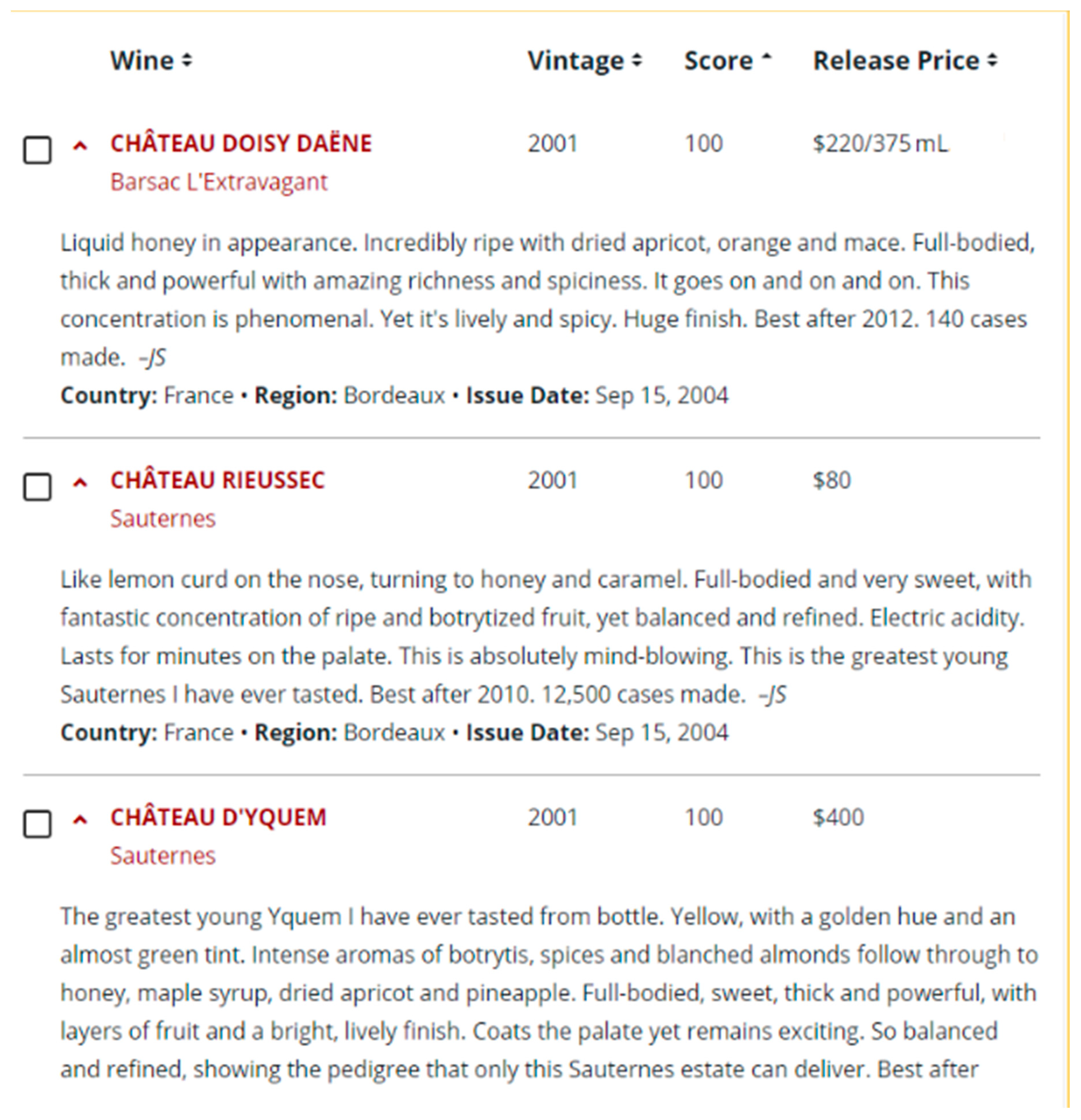
2.1. Wine Spectator
- 95–100 Classic: a great wine
- 90–94 Outstanding: a wine of superior character and style
- 85–89 Very good: a wine with special qualities
- 80–84 Good: a solid, well-made wine
- 75–79 Mediocre: a drinkable wine that may have minor flaws
- 50–74 Not recommended
2.2. Bordeaux Datasets
2.3. Supervised Learning Algorithms and Evaluations
2.3.1. Naïve Bayes Classifier
2.3.2. SVM
2.4. Evaluation Methods
- TP: The real condition is true (1) and predicted as true (1); 90+ wine correctly classified as 90+ wine;
- TN: The real condition is false (−1) and predicted as false (−1); 89− wine correctly classified as 89− wine;
- FP: The real condition is false (−1) but predicted as true (1); 89− wine incorrectly classified as 90+ wine;
- FN: The real condition is true (1) but predicted as false (−1); 90+ wine incorrectly classified as 89− wine;
3. Results and Discussion
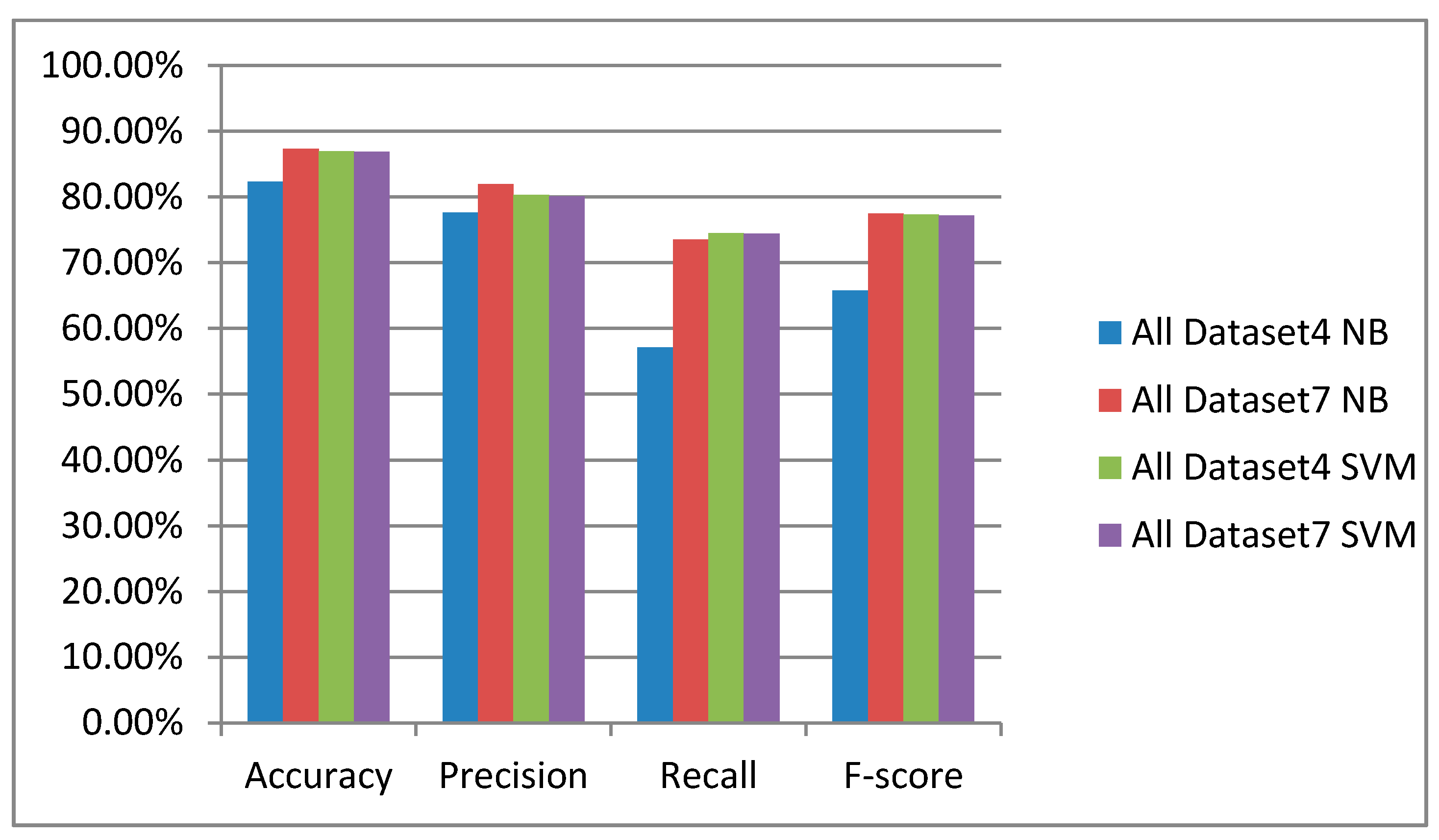
3.1. Results of All Bordeaux Wine Datasets
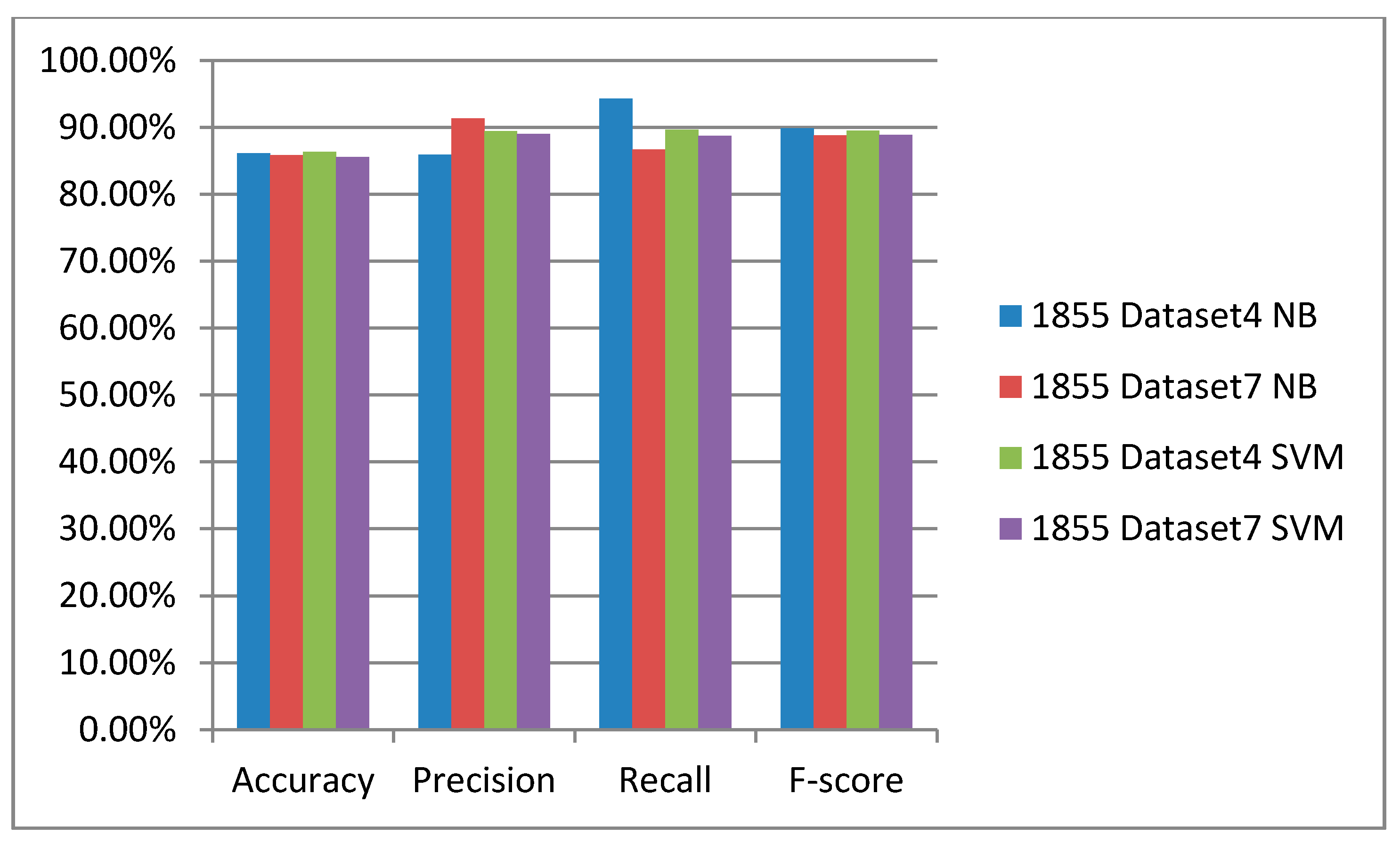
3.2. Results of 1855 Bordeaux Wine Official Classification Dataset
3.3. Comparison of Datasets 4 and 7
4. Conclusions
Author Contributions
Funding
Acknowledgments
Conflicts of Interest
References
- Caruana, R.; Niculescu-Mizil, A. An empirical comparison of supervised learning algorithms. In Proceedings of the 23rd International Conference on Machine Learning, Ser. ICML’06, Pittsburgh, PA, USA, 25–29 June 2006; pp. 161–168. [Google Scholar]
- Hastie, T.; Tibshirani, R.; Friedman, J. Unsupervised Learning; Springer: New York, NY, USA, 2009; pp. 485–585. [Google Scholar]
- Zhu, X.; Goldberg, A.B. Introduction to semi-supervised learning. Synth. Lect. Artif. Intell. Mach. Learn. 2009, 3, 1–130. [Google Scholar] [CrossRef]
- Levine, S. Reinforcement learning and control as probabilistic inference: Tutorial and review. arXiv 2018, arXiv:1805.00909. [Google Scholar]
- Karlsson, P. World Wine Production Reaches Record Level in 2018, Consumption is Stable. BKWine Magazine. 2019. Available online: https://www.bkwine.com/features/more/world-wine-production-reaches-record-level-2018-consumption-stable/ (accessed on 1 January 2021).
- Robert Parker Wine Advocate. Available online: https://www.robertparker.com/ (accessed on 1 January 2020).
- James Suckling Wine Ratings. Available online: https://www.jamessuckling.com/tag/wine-ratings/ (accessed on 1 January 2020).
- Wine Spectator. Available online: https://www.winespectator.com (accessed on 1 January 2020).
- Wine Enthusiast. Available online: https://www.wineenthusiast.com/ (accessed on 1 January 2020).
- Decanter. Available online: https://www.decanter.com/ (accessed on 1 January 2020).
- Chen, B.; Velchev, V.; Palmer, J.; Atkison, T. Wineinformatics: A Quantitative Analysis of Wine Reviewers. Fermentation 2018, 4, 82. [Google Scholar] [CrossRef]
- Palmer, J.; Chen, B. Wineinformatics: Regression on the Grade and Price of Wines through Their Sensory Attributes. Fermentation 2018, 4, 84. [Google Scholar] [CrossRef]
- Cortez, P.; Cerdeira, A.; Almeida, F.; Matos, T.; Reis, J. Modeling wine preferences by data mining from physicochemical properties. Decis. Support Syst. 2009, 47, 547–553. [Google Scholar] [CrossRef]
- Edelmann, A.; Diewok, J.; Schuster, K.C.; Lendl, B. Rapid method for the discrimination of red wine cultivars based on mid-infrared spectroscopy of phenolic wine extracts. J. Agric. Food Chem. 2001, 49, 1139–1145. [Google Scholar] [CrossRef]
- Chen, B.; Rhodes, C.; Crawford, A.; Hambuchen, L. Wineinformatics: Applying data mining on wine sensory reviews processed by the computational wine wheel. In Proceedings of the 2014 IEEE International Conference on Data Mining Workshop, Shenzhen, China, 14 December 2014; pp. 142–149. [Google Scholar]
- Chen, B.; Rhodes, C.; Yu, A.; Velchev, V. The computational wine wheel 2.0 and the TriMax triclustering in wineinformatics. In Industrial Conference on Data Mining; Springer: Cham, Switzerland, 2016; pp. 223–238. [Google Scholar]
- Johnson, H. World Atlas of Wine, 4th ed.; Octopus Publishing Group Ltd.: London, UK, 1994; p. 13. [Google Scholar]
- History. Available online: https://www.bordeaux.com/us/Our-know-how/History (accessed on 1 January 2021).
- Combris, P.; Lecocq, S.; Visser, M. Estimation of a hedonic price equation for Bordeaux wine: Does quality matter? Econ. J. 1997, 107, 389–402. [Google Scholar] [CrossRef]
- Cardebat, J.M.; Figuet, J. What explains Bordeaux wine prices? Appl. Econ. Lett. 2004, 11, 293–296. [Google Scholar] [CrossRef]
- Ashenfelter, O. Predicting the quality and prices of Bordeaux wine. Econ. J. 2008, 118, F174–F184. [Google Scholar] [CrossRef]
- Shanmuganathan, S.; Sallis, P.; Narayanan, A. Data mining techniques for modelling seasonal climate effects on grapevine yield and wine quality. In Proceedings of the 2010 2nd International Conference on Computational Intelligence, Communication Systems and Networks, Liverpool, UK, 28–30 July 2010; pp. 84–89. [Google Scholar]
- Noy, N.F.; Sintek, M.; Decker, S.; Crubézy, M.; Fergerson, R.W.; Musen, M.A. Creating semantic web contents with protege-2000. IEEE Intell. Syst. 2001, 16, 60–71. [Google Scholar] [CrossRef]
- Noy, F.N.; McGuinness, D.L. Ontology Development 101: A Guide to Creating Your First Ontology. Stanford Knowledge Systems Laboratory Technical Report KSL-01-05 and Stanford Medical Informatics Technical Report SMI-2001-0880. 2001. Available online: http://www.ksl.stanford.edu/people/dlm/papers/ontology-tutorial-noy-mcguinness-abstract.html (accessed on 1 January 2021).
- Quandt, R.E. A note on a test for the sum of rank sums. J. Wine Econ. 2007, 2, 98–102. [Google Scholar] [CrossRef]
- Ashton, R.H. Improving experts’ wine quality judgments: Two heads are better than one. J. Wine Econ. 2011, 6, 135–159. [Google Scholar] [CrossRef]
- Ashton, R.H. Reliability and consensus of experienced wine judges: Expertise within and between? J. Wine Econ. 2012, 7, 70–87. [Google Scholar] [CrossRef]
- Bodington, J.C. Evaluating wine-tasting results and randomness with a mixture of rank preference models. J. Wine Econ. 2015, 10, 31–46. [Google Scholar] [CrossRef]
- Dong, Z.; Guo, X.; Rajana, S.; Chen, B. Understanding 21st Century Bordeaux Wines from Wine Reviews Using Naïve Bayes Classifier. Beverages 2020, 6, 5. [Google Scholar] [CrossRef]
- Chen, B. Wineinformatics: 21st Century Bordeaux Wines Dataset, IEEE Dataport. 2020. Available online: https://ieee-dataport.org/open-access/wineinformatics-21st-century-bordeaux-wines-dataset (accessed on 1 January 2021).
- Robinson, J. The Oxford Companion to Wine, 3rd ed.; Oxford University Press: Oxford, UK, 2006; pp. 175–177. [Google Scholar]
- Bird, S.; Klein, E.; Loper, E. Natural Language Processing with Python: Analyzing Text with the Natural Language Toolkit; O’Reilly Media, Inc.: Newton, MA, USA, 2009. [Google Scholar]
- Cardebat, J.M.; Livat, F. Wine experts’ rating: A matter of taste? Int. J. Wine Bus. Res. 2016, 28, 43–58. [Google Scholar] [CrossRef]
- Cardebat, J.M.; Figuet, J.M.; Paroissien, E. Expert opinion and Bordeaux wine prices: An attempt to correct biases in subjective judgments. J. Wine Econ. 2014, 9, 282–303. [Google Scholar] [CrossRef]
- Cao, J.; Stokes, L. Evaluation of wine judge performance through three characteristics: Bias, discrimination, and variation. J. Wine Econ. 2010, 5, 132–142. [Google Scholar] [CrossRef]
- Cardebat, J.M.; Paroissien, E. Standardizing expert wine scores: An application for Bordeaux en primeur. J. Wine Econ. 2015, 10, 329–348. [Google Scholar] [CrossRef]
- Hodgson, R.T. An examination of judge reliability at a major US wine competition. J. Wine Econ. 2008, 3, 105–113. [Google Scholar] [CrossRef]
- Hodgson, R.T. An analysis of the concordance among 13 US wine competitions. J. Wine Econ. 2009, 4, 1–9. [Google Scholar] [CrossRef]
- Hodgson, R.; Cao, J. Criteria for accrediting expert wine judges. J. Wine Econ. 2014, 9, 62–74. [Google Scholar] [CrossRef]
- Hopfer, H.; Heymann, H. Judging wine quality: Do we need experts, consumers or trained panelists? Food Qual. Prefer. 2014, 32, 221–233. [Google Scholar] [CrossRef]
- Li, W.; Liu, Z. A method of SVM with Normalization in Intrusion Detection. Procedia Environ. Sci. 2011, 11, 256–262. [Google Scholar] [CrossRef]
- Metsis, V.; Androutsopoulos, I.; Paliouras, G. Spam Filtering with Naive Bayes—Which Naive Bayes? In Proceedings of the CEAS, Mountain View, CA, USA, 27–28 July 2018.
- Rish, I. An empirical study of the naive Bayes classifier. In Proceedings of the IJCAI 2001 Workshop on Empirical Methods in Artificial Intelligence, Seattle, WA, USA, 4–10 August 2001; Volume 3, pp. 41–46. [Google Scholar]
- Lou, W.; Wang, X.; Chen, F.; Chen, Y.; Jiang, B.; Zhang, H. Sequence based prediction of DNA-binding proteins based on hybrid feature selection using random forest and Gaussian naive Bayes. PLoS ONE 2014, 9, e86703. [Google Scholar] [CrossRef]
- Narayanan, V.; Arora, I.; Bhatia, A. Fast and accurate sentiment classification using an enhanced Naive Bayes model. In International Conference on Intelligent Data Engineering and Automated Learning; Springer: Berlin/Heidelberg, Germany, 2013; pp. 194–201. [Google Scholar]
- Suykens, K.J.A.; Vandewalle, J. Least squares support vector machine classifiers. Neural Process. Lett. 1999, 9, 293–300. [Google Scholar] [CrossRef]
- Thorsten, J. Svmlight: Support Vector Machine. Available online: https://www.researchgate.net/profile/Thorsten_Joachims/publication/243763293_SVMLight_Support_Vector_Machine/links/5b0eb5c2a6fdcc80995ac3d5/SVMLight-Support-Vector-Machine.pdf (accessed on 1 January 2020).
- Chen, B.; Velchev, V.; Nicholson, B.; Garrison, J.; Iwamura, M.; Battisto, R. Wineinformatics: Uncork Napa’s Cabernet Sauvignon by Association Rule Based Classification. In Proceedings of the 2015 IEEE 14th International Conference on Machine Learning and Applications (ICMLA), Miami, FL, USA, 9–11 December 2015; pp. 565–569. [Google Scholar]
- Chen, B.; Jones, D.; Tunc, M.; Chipolla, K.; Beltrán, J. Weather Impacts on Wine, A BiMax examination of Napa Cabernet in 2011 and 2012 Vintage. In Proceedings of the ICDM 2019, New York, NY, USA, 17–21 July 2019; pp. 242–250. [Google Scholar]
- Palmer, J.; Sheng, V.S.; Atkison, T.; Chen, B. Classification on grade, price, and region with multi-label and multi-target methods in wineinformatics. Big Data Min. Anal. 2019, 3, 1–12. [Google Scholar] [CrossRef]


| CATEGORY_NAME | SUBCATEGORY_NAME | SPECIFIC_NAME | NORMALIZED_NAME |
|---|---|---|---|
| CARAMEL | CARAMEL | 71 | 40 |
| CHEMICAL | PETROLEUM | 9 | 5 |
| SULFUR | 11 | 10 | |
| PUNGENT | 4 | 3 | |
| EARTHY | EARTHY | 72 | 31 |
| MOLDY | 2 | 2 | |
| FLORAL | FLORAL | 61 | 39 |
| FRUITY | BERRY | 49 | 28 |
| CITRUS | 37 | 23 | |
| DRIED FRUIT | 67 | 60 | |
| FRUIT | 22 | 9 | |
| OTHER | 25 | 18 | |
| TREE FRUIT | 39 | 31 | |
| TROPICAL FRUIT | 48 | 27 | |
| FRESH | FRESH | 41 | 29 |
| DRIED | 25 | 21 | |
| CANNED/COOKED | 16 | 15 | |
| MEAT | MEAT | 25 | 13 |
| MICROBIOLOGICAL | YEASTY | 5 | 4 |
| LACTIC | 14 | 6 | |
| NUTTY | NUTTY | 25 | 15 |
| OVERALL | TANNINS | 90 | 4 |
| BODY | 50 | 23 | |
| STRUCTURE | 40 | 2 | |
| ACIDITY | 40 | 3 | |
| FINISH | 184 | 5 | |
| FLAVOR/DESCRIPTORS | 649 | 432 | |
| OXIDIZED | OXIDIZED | 1 | 1 |
| PUNGENT | HOT | 3 | 2 |
| COLD | 1 | 1 | |
| SPICY | SPICE | 83 | 44 |
| WOODY | RESINOUS | 24 | 9 |
| PHENOLIC | 6 | 4 | |
| BURNED | 47 | 26 |
| All Bordeaux Datasets (14,349 Wines) | 1855 Bordeaux Datasets (1359 Wines) | Attributes Used in the Dataset |
|---|---|---|
| 1 | 1 | 14 category attributes |
| 2 | 2 | 34 subcategory attributes |
| 3 | 3 | 985 normalized attributes |
| 4 | 4 | 14 category attributes + 34 subcategory attributes + 985 normalized attributes |
| 5 | 5 | 14 category attributes + 34 subcategory attributes |
| 6 | 6 | 34 subcategory attributes + 985 normalized attributes |
| 7 | 7 | 14 category attributes + 985 normalized attributes |
| All Bordeaux Dataset | Accuracy | Precision | Recall | F-Score |
|---|---|---|---|---|
| 1 | 74.39% | 61.64% | 36.48% | 45.83% |
| 2 | 74.72% | 61.17% | 40.86% | 48.98% |
| 3 | 85.17% | 73.22% | 79.03% | 76.01% |
| 4 | 82.37% | 77.65% | 57.10% | 65.80% |
| 5 | 74.93% | 62.09% | 40.11% | 48.73% |
| 6 | 84.79% | 81.32% | 63.38% | 71.22% |
| 7 | 87.32% | 81.94% | 73.52% | 77.49% |
| All Bordeaux Dataset | Accuracy | Precision | Recall | F-Score |
|---|---|---|---|---|
| 1 | 80.46% | 73.31% | 53.81% | 62.06% |
| 2 | 82.09% | 75.58% | 58.67% | 66.06% |
| 3 | 86.97% | 80.68% | 73.80% | 77.10% |
| 4 | 87.00% | 80.35% | 74.50% | 77.31% |
| 5 | 82.12% | 75.53% | 58.88% | 66.17% |
| 6 | 87.00% | 80.31% | 74.53% | 77.30% |
| 7 | 86.92% | 80.13% | 74.45% | 77.18% |
| 1855 Bordeaux Dataset | Accuracy | Precision | Recall | F-Score |
|---|---|---|---|---|
| 1 | 70.36% | 77.15% | 78.21% | 77.37% |
| 2 | 71.97% | 75.10% | 85.73% | 79.91% |
| 3 | 84.62% | 86.79% | 90.02% | 88.38% |
| 4 | 86.18% | 85.92% | 94.33% | 89.89% |
| 5 | 76.02% | 76.08% | 92.63% | 83.43% |
| 6 | 86.17% | 86.54% | 93.31% | 89.78% |
| 7 | 85.88% | 91.34% | 86.72% | 88.84% |
| 1855 Bordeaux Dataset | Accuracy | Precision | Recall | F-Score |
|---|---|---|---|---|
| 1 | 71.22% | 73.94% | 86.17% | 79.55% |
| 2 | 79.18% | 82.17% | 86.74% | 84.37% |
| 3 | 81.38% | 86.84% | 84.12% | 85.46% |
| 4 | 86.38% | 89.42% | 89.68% | 89.53% |
| 5 | 85.58% | 86.47% | 92.29% | 89.26% |
| 6 | 82.48% | 86.67% | 86.28% | 86.46% |
| 7 | 85.57% | 89.05% | 88.77% | 88.89% |
Publisher’s Note: MDPI stays neutral with regard to jurisdictional claims in published maps and institutional affiliations. |
© 2021 by the authors. Licensee MDPI, Basel, Switzerland. This article is an open access article distributed under the terms and conditions of the Creative Commons Attribution (CC BY) license (http://creativecommons.org/licenses/by/4.0/).
Share and Cite
Dong, Z.; Atkison, T.; Chen, B. Wineinformatics: Using the Full Power of the Computational Wine Wheel to Understand 21st Century Bordeaux Wines from the Reviews. Beverages 2021, 7, 3. https://doi.org/10.3390/beverages7010003
Dong Z, Atkison T, Chen B. Wineinformatics: Using the Full Power of the Computational Wine Wheel to Understand 21st Century Bordeaux Wines from the Reviews. Beverages. 2021; 7(1):3. https://doi.org/10.3390/beverages7010003
Chicago/Turabian StyleDong, Zeqing, Travis Atkison, and Bernard Chen. 2021. "Wineinformatics: Using the Full Power of the Computational Wine Wheel to Understand 21st Century Bordeaux Wines from the Reviews" Beverages 7, no. 1: 3. https://doi.org/10.3390/beverages7010003
APA StyleDong, Z., Atkison, T., & Chen, B. (2021). Wineinformatics: Using the Full Power of the Computational Wine Wheel to Understand 21st Century Bordeaux Wines from the Reviews. Beverages, 7(1), 3. https://doi.org/10.3390/beverages7010003