1. Introduction
A variable annuity (VA) is a popular life insurance product created by insurance companies to address many people’s concerns about outliving their assets [
1,
2]. Under a VA policy, the policyholder agrees to make a lump-sum or a series of purchase payments to the insurer and in return the insurer agrees to make benefit payments to the policyholder, beginning either immediately or on a future date. Policyholders choose to invest their money in one or more investment funds provided by the insurance company. A main feature of VAs is that they come with guarantees or riders, which are designed to protect the policyholder’s capital against market downturns.
There are two types of guaranteed benefits embedded in VA policies: death benefits and living benefits. A guaranteed minimum death benefit (GMDB) guarantees a specified amount to the beneficiary upon the death of the policyholder regardless of the performance of the investment portfolio. Examples of living benefits include the guaranteed minimum withdrawal benefit (GMWB), the guaranteed minimum income benefit (GMIB), the guaranteed minimum maturity benefit (GMMB), and the guaranteed minimum accumulation benefit (GMAB). A GMWB guarantees that the policyholder can take systematic annual withdrawals of a specified amount from the policy over a period of time, even though the investment portfolio might be depleted. A GMIB guarantees that the policyholder can convert the VA policy to an annuity according to a specified rate. A GMMB guarantees that the policyholder can receive a specific amount at the maturity of the policy. A GMAB guarantees that the policyholder can renew the contract during a specified window after a specified waiting period.
Due to these attractive guarantees, many VA policies were sold in the past two decades.
Figure 1 shows the annual VA sales in the United States during the period from 2008 to 2017. In the figure, we see that, except for 2017, the annual sales in all these years were above
$100 billion. The guarantees embedded in VA policies are financial guarantees and cannot be adequately addressed by traditional actuarial methods [
3]. To mitigate the financial risks associated with the VA guarantees, many insurance companies with a VA business have adopted dynamic hedging [
4,
5].
To simulate the performance of dynamic hedging for VA products, insurance companies rely on nested stochastic projections [
5]. Nested stochastic projections are also referred to as “stochastic on stochastic” projections.
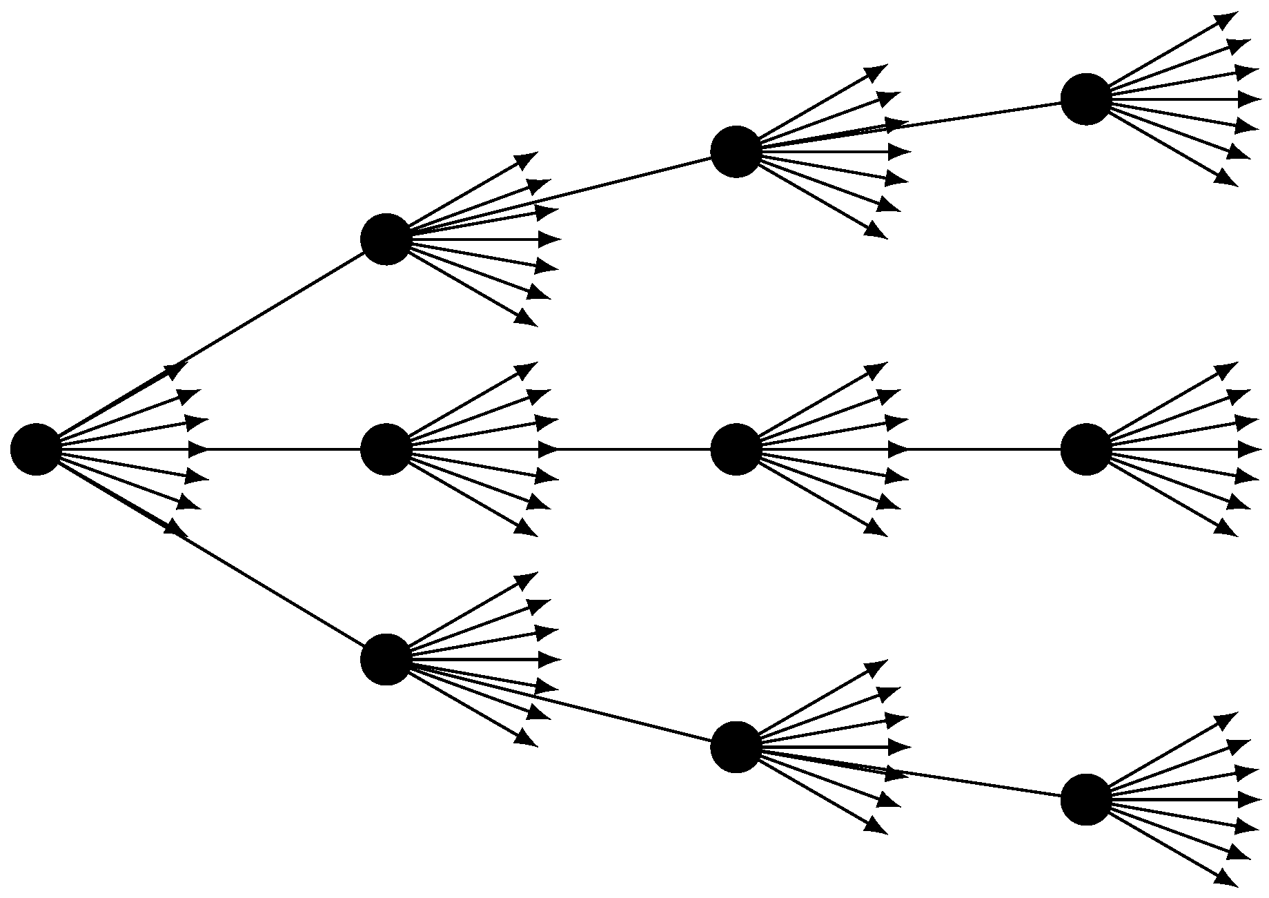
Figure 2 conceptualizes the structure of a typical nested stochastic projection, which involves two layers of stochastic projections. At each node of an outer stochastic path, a set of inner stochastic paths is embedded. Usually the outer stochastic paths are real-world scenarios, which reflect a realistic pattern of underlying market prices that are used to generate realistic distributions of outcomes. In contrast, the inner stochastic paths are risk-neutral scenarios, which use unrealistic assumptions about risk premiums for purposes of calculating derivative prices under the no-arbitrage assumption.
The computation of nested stochastic projections for a large VA portfolio is highly computationally intensive and often prohibitive because every policy in the portfolio needs to be projected over many paths for a long time horizon [
6]. For example, if we use 1000 real-world scenarios in the outer layer and 1000 risk-neutral paths in the inner layer, and project the cash flows at yearly steps for 30 years, then the total number of projections for each policy is
which is already a big number. For a portfolio of 100,000 contracts, the number of projections would be
. Suppose that a single CPU can process 200,000 cash flow projections in a second. Then, it will take this CPU
years to process all the cash flow projections for the portfolio. The amount of time shown in the above equation is just the runtime used to project the cash flows once. To calculate the Greeks, we need to project the cash flows multiple times at different shocks of the market. This will increase the runtime multifold.
Recently, metamodeling approaches have been proposed to address the computational issues associated with the valuation of large VA portfolios (see, for example, [
7,
8,
9,
10,
11,
12,
13,
14,
15,
16]). The main idea of these metamodeling approaches is to build a predictive model based on a set of representative VA policies and their fair market values (or other quantities of interest). The predictive model is then used to estimate the fair market values for all the policies in the portfolio. This can reduce the number of policies that are valued by Monte Carlo simulation. Since predictive models are usually much faster than Monte Carlo simulation, the gain in valuation runtime is significant.
However, it is difficult for academic researchers to obtain real datasets from insurance companies to assess the performance of metamodeling techniques. In this paper, we create synthetic datasets that can be used by researchers and practitioners to test metamodeling methods for the efficient valuation of large VA portfolios under nested stochastic simulation. In particular, we implement a nested stochastic valuation engine that is used to calculate the Greeks for VA policies along outer layer paths. The purpose of this work is to relieve researchers from spending time on creating such datasets, which can be extremely time-consuming to create. This paper differs from a previous paper [
10] in that this paper focuses on developing comprehensive synthetic datasets while the previous paper focuses on metamodeling. This paper also differs from the paper [
17] because this paper is about creating synthetic datasets under the stochastic-on-stochastic valuation framework while the paper [
17] is about creating synthetic datasets for valuation only at time zero.
The remaining part of this paper is structured as follows.
Section 2 presents a nested stochastic simulation engine for valuing the guarantees embedded in variable annuities. In
Section 3 and
Section 4, we present synthetic datasets that can be used to test the performance of metamodeling techniques. In
Section 5, we conclude the paper with some remarks. The software that implements the nested Monte Carlo simulation engine is described in
Appendix A.
2. Nested Stochastic Valuation
In this section, we describe the nested stochastic valuation engine. In particular, we introduce the risk-neutral scenario generator, the real-world scenario generator, and the cash flow projections.
2.1. Risk-Neutral Scenario Generator
Risk-neutral scenarios are used in the inner loop to calculate the dollar Deltas. We use a multivariate Black–Scholes model introduced by Carmona and Durrelman [
18] to generate risk-neutral scenarios. This model is also described in [
17].
Let
,
, …,
be
k indices in the financial market. Under the multivariate Black–Scholes model, the risk-neutral dynamics of the
k indices are given by [
18]:
or
where
,
, …,
are independent standard Brownian motions,
is the short rate of interest, and the matrix
is used to capture the correlation among the indices.
Let
be time steps with equal space
and suppose that the continuous forward rate is constant within each period. For
, the accumulation factor of the
hth index for the period
can be calculated as:
where
is the annualized continuous forward rate for period
and
By the property of Brownian motion, we know that , , …, are independent random variables with a standard normal distribution.
The continuous return for the period
is calculated as:
The matrix
can be obtained from the following Cholesky decomposition of the covariance matrix
:
where
is a vector of index volatilities,
is a diagonal matrix with
as diagonal elements, and
is the correlation matrix. In matrix form, Equation (
4) can be expressed as
Algorithm 1 shows the pseudo-code of the risk-neutral scenario generator. Once we have index scenarios simulated from Equation (
3), we can obtain the investment fund scenarios by blending these index scenarios as follows:
where
g is the number of investment funds and
is the fund mapping that maps the
k indices to the
g investment funds.
| Algorithm 1: Pseudo-code of the Risk-neutral Scenario Generator. |
![Data 03 00031 i001]() |
2.2. Real-World Scenario Generator
Real-world scenarios are used in the outer loop to simulate the movements of the market. Risk-neutral scenarios are prospective and parameters of the risk-neutral scenario generator are calibrated to market data. Real-world scenarios are retrospective and the parameters of a real-world scenario generator are calibrated to historical data.
In practice, the regime-switching model [
19] is typically used to generate real-world scenarios. Here, we introduce a multivariate two-regime regime-switching model for generating correlated real-world scenarios for multiple indices. Within a regime and a time period, the evolution of the indices follows the multivariate log-normal model.
Let
denote the regime at time
t and
M denote the transition matrix, i.e.,
where
Let
be the unconditional probability distribution of the regime-switching process. Then, we have
which gives [
19]:
Let
,
, …,
be
k indices in the financial market. Under the multivariate two-regime regime-switching log-normal model, the risk-world dynamics of the
k indices are given by:
where
,
, …,
are independent standard Brownian motions,
is the geometric mean of the
hth index in the regime
, the matrix
is used to capture the correlation among the indices in the regime
, and
is the regime number.
Let
,
, …,
be time steps, where
is the time step. Then, for
, the accumulation factor of the
hth index for the period
in the regime
can be calculated as
where
In matrix form, the returns can be expressed as
where the matrix
can be obtained from the following Cholesky decomposition of the covariance matrix
:
where
is a vector of index volatilities for regime
,
is a diagonal matrix with
as diagonal elements, and
is the correlation matrix for regime
.
Let
be the initial regime. Then, for
, the regime for period
j can be determined by generating a uniform random number
u as follows:
The continuous return of the
hth index for the period
in the regime
is calculated
Algorithm 2 shows the pseudo-code of the two-regime regime-switching real-world scenario generator.
| Algorithm 2: Pseudo-code of the Two-regime Regime-switching Real-world Scenario Generator. |
![Data 03 00031 i002]() |
From the above equation, we can derive the expectations and covariances of the conditioned returns as follows:
and
The return of the
hth index for the period
can be expressed as
where
I is an indicator function.
The expected return for the period
can be calculated as p177 in [
20]:
From Equation (
14), we have
which gives
Letting
in the above equation, we get the variance of the return as follows:
where
is the volatility of the
hth index in the regime
, i.e.,
Equations (
15) and (
17) can be used to validate the real-world scenarios. These equations can also be used to specify parameters for the two-regime regime-switching model if we want to control the overall mean returns and the overall volatilities of the indices.
2.3. Nested Stochastic Valuation
To describe how nested stochastic projections are done, we let
be the number of outer loop paths and let
be the number of time nodes in the outer loop. Let
be a portfolio of
n VA policies. Algorithm 3 shows a high-level sketch of the nested stochastic valuation engine. At each node along each outer loop path, we calculate the fair market values of each policy using the risk-neutral scenarios. For details about how policies are aged along a real-world path and how the cash flows are projected along a risk-neutral path, readers are referred to [
17].
| Algorithm 3: A High-level Sketch of the Nested Stochastic Valuation Engine. |
![Data 03 00031 i003]() |
To assess the performance of dynamic hedging, partial dollar deltas are required as hedging is done by individual tradable indices. The partial dollar delta on the
hth index is normally calculated as follows:
where
denotes the account value invested in the
hth index. However, calculating partial dollar deltas using the above equation requires projecting cash flows at many index shocks. This is prohibitive under the nested stochastic valuation framework.
To reduce the runtime, we only calculate total dollar delta at each node along an outer loop path as follows:
where
k is the number of indices. Then, we approximate the partial dollar deltas as follows:
The relation given in Equation (
18) can be derived as follows. Suppose that the fair market value of the guarantees embedded in a VA policy is a function of the total account value, i.e.,
Then, the partial dollar delta on the
hth index is calculated as
where
is the total account value.
4. Partial Dollar Deltas
In this section, we present the partial dollar deltas calculated by the nested Monte Carlo simulation method described in
Section 2.
As discussed in
Section 2, the nested stochastic valuation program produces many matrices of the partial dollar deltas. In fact, the program produces
matrices of partial dollar deltas, where
is the number of real-world paths and
H is the number of indices. For
and
, let
be the matrix of the partial dollar deltas on the
hth index:
where
n is the number of policies in the portfolio,
T is the number of time points where partial dollar deltas are calculated, and
denotes the partial dollar delta of the
ith policy on the
hth index at
jth evaluation time point along the
pth real-world path. Since we used
real-world paths and
evaluation time points and the number of indices is
, the number of matrices we produced is 5000. Each matrix has a size of
. We saved all the matrices to CSV files with only six decimal places. If zip all the CSV files, the size of the zip file is around 20 GB.
4.1. Aggregate Results
The aggregate partial dollar deltas along a real-world path are calculated as follows:
In other words, the aggregate partial dollar deltas are the partial dollar deltas of the whole portfolio. The aggregate total dollar deltas are calculated as
Figure 7 shows the aggregate partial dollar deltas and aggregate total dollar deltas along the 1000 real-world paths. In the figure, we have the following observations:
The aggregate partial dollar deltas do not approach zero at the end of the projection horizon. This is caused by the GMAB products, which behave similar to call options.
The guarantees are more sensitive to indices with higher volatilities. For example, the magnitudes of the aggregate partial dollar deltas on the small cap equity are larger than those on other indices.
The aggregate total dollar deltas along the best and the worst real-world paths have similar magnitudes. This is because the dollar deltas of the GMAB product offset those of other products.
For equity indices, which have high volatilities, the aggregate partial dollar deltas have similar magnitudes along the best and the worst real-world paths. For non-equity indices, which have low volatilities, the aggregate partial dollar deltas along the worst real-world path have higher magnitudes than those along the best real-world path.
Figure 8 and
Figure 9 show the histograms of the aggregate partial dollar deltas at the Year 1 and the Year 30, respectively. In the figures, we see that the distributions of the aggregate partial dollar deltas at the Year 30 is more skewed that those at the Year 1.
4.2. Seriatim Results
There are many seriatim results, making it difficult to show all the results in detail. In this section, we only show the seriatim results from the best and the worst real-world paths identified before.
Figure 10 shows a histogram of the seriatim partial dollar deltas at the end of Year 1 if the best real-world path occurs.
Figure 11 shows a similar histogram if the worst real-world path occurs. Both figures show that the distributions of the seriatim partial dollar deltas are highly skewed. In addition, some policies have positive dollar deltas if the best real-world path occurs. This is caused by the GMAB products as a bull market can trigger the renew option embedded in such products.
Figure 12 and
Figure 13 show the box plots of seriatim partial dollar deltas by product type at the end of Year 1 along the best and the worst real-world paths, respectively. In these figures, we see that the GMAB, GMIB, and GMMB products are more sensitive than the GMDB and GMWB products in terms of the magnitudes of the deltas. In addition, more policies have positive deltas when the best real-world path occurs than the case when the worst real-world path occurs.
4.3. Runtime
We implemented the nested stochastic valuation engine as a distributed multi-threading program in Java. We used the HPC (High Performance Computing) cluster (
https://hpc.uconn.edu/) at the University of Connecticut to run the program. In particular, we used eight instances of the program with 20 cores for each instance to calculate the partial dollar deltas for the portfolio. Each instance of the program handles one outer loop path at a time. The coordination between different instances is done via the mechanism of file locking. Even with 160 cores, it took about two weeks to get all the calculations done.
For the convenience of comparison, we accumulate the runtime used by all threads to get the runtime that would be used by a single core.
Figure 14 shows a histogram of the runtime used to calculate the partial dollar deltas for an outer loop path. In the figure, we see that, if a single core is used, it would take the core about 20–32 h to finish the calculation for a single outer loop path. If we aggregate the runtime used to process all 1000 outer loop paths, the runtime is 93,722,002.966 s or 2.97 years. In other words, if we used a single CPU to calculate the partial dollar deltas for the portfolio of 38,000 VA policies with 1000 real-world path and 1000 risk-neutral paths, it would take this CPU about 2.97 years to finish the calculation. Note that we only calculated the partial dollar deltas at 30 time points along the outer loop paths. If we want to calculate the deltas at 360 time points along the outer loop paths, it would take a single core about 36 years.
5. Concluding Remarks
Metamodeling techniques have been proposed to address the computational issues associated with the nested stochastic valuation of large VA portfolios. However, it is difficult for researchers to obtain real datasets from insurance companies to test the metamodeling techniques and publish the results in academic journals. It is the primary purpose of this paper to create synthetic datasets to address computational issues. These synthetic datasets can be used by researchers and practitioners to test techniques, especially metamodeling techniques, to speed up the nested stochastic valuation of large VA portfolios.
These synthetic datasets have some limitations. First, the synthetic VA policies are simpler than VA policies sold in the real-world. Second, the Monte Carlo simulation is also simpler than the one used in practice. For example, we did not consider the policyholder behavior in the cash flow projections. Although the synthetic datasets have limitations, we can still use them to test metamodeling techniques. If a metamodeling technique does not work for the synthetic datasets, then it is unlikely to work for real datasets.


