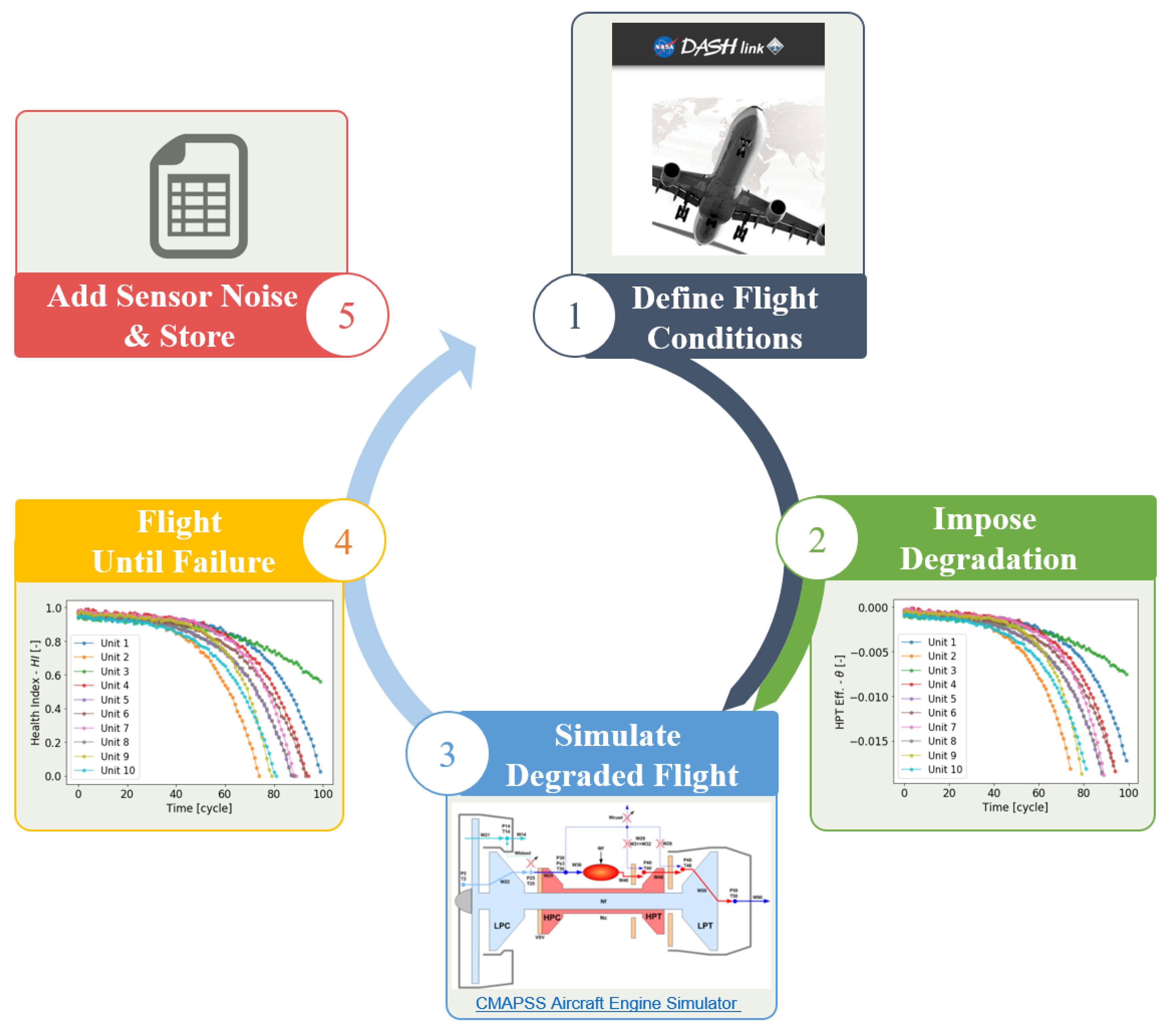
In the following, we describe the key steps of the data generation process outlined above in more detail.
3.1. Degradation Model
The degradation of each engine is modelled as the combination of three contributors: an initial degradation, a normal degradation and abnormal degradation. The dataset generation process assumes failure modes exhibiting a continuous degradation of the main rotating engine sub-components: fan, LPC, HPC, HPT and LPT. The degradation effects are modelled by adjustments of flow capacity and efficiency of these engine sub-components (i.e., the engine health parameters ).
Initial degradation. Due to manufacturing and assembly tolerances, each unit of the fleet has sightly different initial wear at the engine sub-component. Degradation due to this initial wear is not considered abnormal but can make a difference in useful operational life of a component. Following the original work, this initial wear is modeled by variations in flow and efficiencies of the various sub-component. An uniform random distribution is assumed for each of the sub-components. The magnitude of such variations is relatively low, resulting in a health index within the range [0.9 to 1.0]. We denote the initial degradation as .
Normal degradation. In addition to the initial wear, the system’s components also experience degradation due to wear and tear resulting from usage. This type of degradation is considered normal and is modelled as linear decreasing trend given by:
where
is the slope of the degradation, and
t refers to the time in units of cycles, i.e., flights.
Transition from normal to abnormal degradation. Some time during an engine’s life, its health state might transition to an
abnormal state resulting from the presence of a particular failure mode. That is, at a point in time,
, the corresponding fault leads to an
abnormal condition and to an eventual failure at
(i.e., end-of-life). We model the onset of a fault as a stochastic process governed by past operation history. While the detailed computation of the micro-level processes leading to a degraded state was not within the scope of this analysis, we capture the macro-level degradation characteristics leading to a fault by computing the energy balances around each sub-component. Concretely, it is assumed that each sub-component can only withstand certain excitation energy before reaching a state of abnormal degradation. We denote the maximum excitation energy of sub-component
as
, which we model as a Gaussian distribution to represent variability on the material properties of each unit. The fault onset time corresponds to the point in time at which the total amount of energy
E that a component has been exited with from an initial time
to a time
t exceeds
. i.e.,
. The excitation energy experienced by a sub-component in the time interval
is given by:
where
is the power consumed or produced by each component.
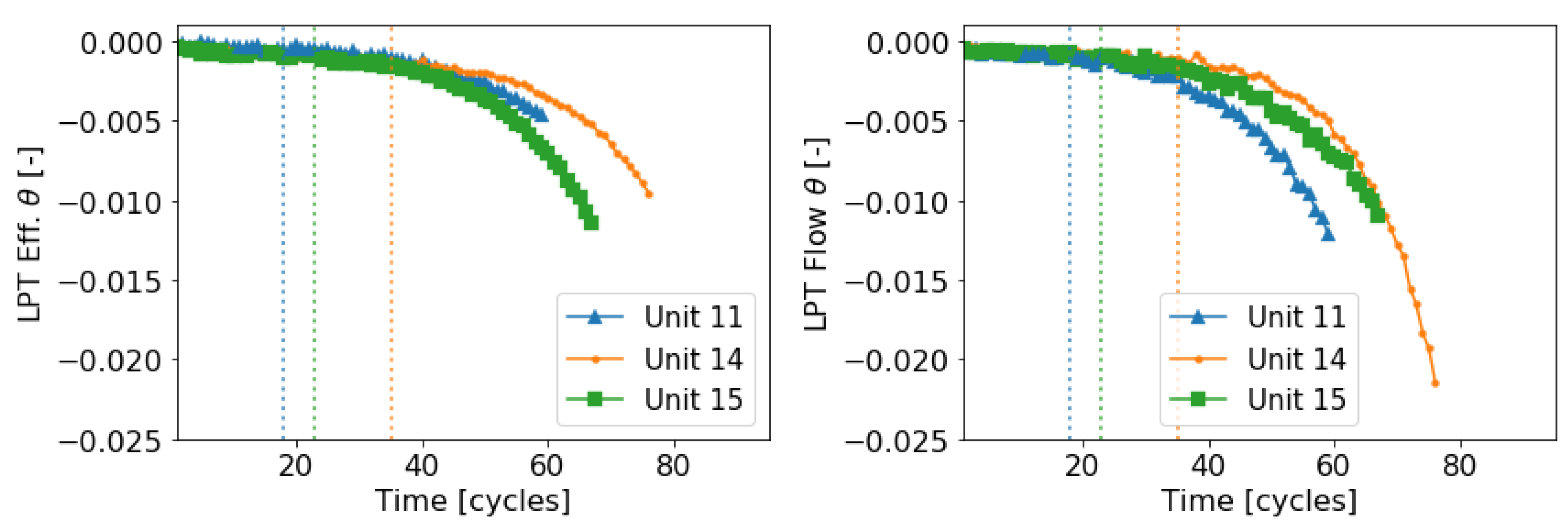
Abnormal degradation. The evolution of the abnormal system degradation with time follows the modelling of the original work. In brief, the abnormal degradation model assumes the degradation of each system sub-components flow and efficiencies (i.e.,
) is governed by the following model:
where
,
and
is the process noise with
when
corresponds to an efficiency and
to a flow capacity.
Since
a,
b and
are random variables, the evolution of the abnormal degradation with time is stochastic. The degradation process follows an exponential behaviour common in multiple damage propagation models (e.g., Arrhenius, Coffin–Manson, and Eyring models). Concretely, the modelling assumes a generalized equation for wear,
, which ignores micro-level deterioration processes but retains macro-level degradation characteristics. The between-flight maintenance is not explicitly modeled but is considered by the process noise. This allows the engine health parameters (flow and efficiency) to improve within allowable limits at any point and hence the loss in efficiency or flow is not locally monotonic (see step 2 in
Figure 1).
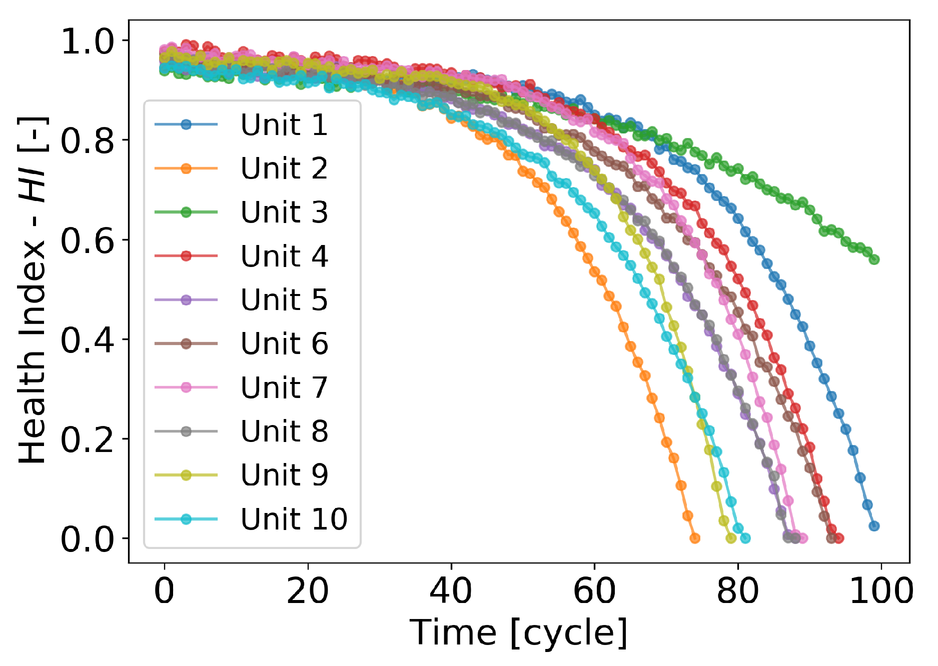
3.2. Health Condition
The modelling approach assumes an overall health index of the engine i.e.,
. The health index of the engine is monitored at each flight, and the end of life is declared when the health index reaches a zero value i.e.,
or the system has reached more that 100 operative cycles. The overall health index is modelled as aggregation of four normalized remaining operative margins (
) that characterize the wear/health of the engine:
In particular, the surge margins of the fan (
), LPC (
) and HPC (
) and the exhaust gas temperature (
) computed at reference conditions
2 are the operative margins considered that we denote as
. Delta differences of these operative margins between a degraded engine and the corresponding values of a clean new engine are assumed as measures of wear i.e.,
. Furthermore, the degradation model assumes upper wear thresholds,
, that denote the operational limits beyond which the engine cannot be operated. Under this assumption, the evolution of the normalized remaining operative margins with time,
, for each of the operative margins monitored is obtained by subtracting the wear from an upper threshold
and normalizing it with respect to the upper threshold:


