Article

Structural Optimization of the Venturi Fertilizer Applicator Using Head Loss Calculation Methods

1
School of Mechanical and Electrical Engineering, Jiangsu Vocational College of Agriculture and Forestry, Zhenjiang 212400, China
2
School of Mechanical Engineering, Jiangsu University of Technology, Changzhou 213001, China
3
Jiangsu Modern Agricultural Equipment and Engineering Center, Zhenjiang 212400, China
4
Research Center of Fluid Machinery and Technology, Jiangsu University, Zhenjiang 212013, China
5
Nanjing Wotian Intelligent Technology Company Limited, Nanjing 210046, China
*
Author to whom correspondence should be addressed.
Fluids 2025, 10(4), 87; https://doi.org/10.3390/fluids10040087
Submission received: 16 February 2025 / Revised: 26 March 2025 / Accepted: 28 March 2025 / Published: 31 March 2025
(This article belongs to the Special Issue Hydraulic Flow in Pipelines)

Abstract

:
Fertilizer suction flow rate is an important performance parameter of the Venturi fertilizer applicator. This study aims to analyze the optimal structure of the Venturi fertilizer applicator with the goal of maximizing the suction flow rate at the same inlet and outlet pressures. A Venturi tube was used as a simplified case for investigating the Venturi injector. A calculation formula for the head loss between the inlet and outlet of the Venturi tube was derived based on the Bernoulli equation and the Darcy–Weisbach formula. Subsequently, it was modified through regression analysis based on the experimental and numerical simulation results of the flow on the Venturi tube. The optimal structure of the Venturi injector was further analyzed based on the head loss calculation formula. The optimal range for the reducing angle and expanding angle of the Venturi injector were determined to be 20–28° and 6–10°, respectively. The optimal throat diameter was identified to be 5–7 mm when the inlet flow rates were within the range of 1.5–2.5 m3/h. The optimum suction pipe diameter and throat pipe length were both equal to the throat diameter.

1. Introduction

The performance of a fertigation system significantly relies on the effectiveness of the fertilization equipment. The Venturi injector, developed based on the Venturi effect, plays a crucial role in this regard. Due to its low cost, ease of operation, and consistent suction flow rate, it is widely employed in drip irrigation [1,2,3]. Some researchers carried out experiments to assess the performance of the Venturi injector. For instance, Sobenko et al. [4] conducted performance tests using water as the suction fluid and proposed a predictive model for the injection flow rate based on their experimental findings. Furthermore, the performance of the Venturi injector in a drip fertigation system was assessed in relation to water and fertilizer uniformity [5]. The uniformity of fertilization using a Venturi injector in a fertigation system was compared with that of a pressure differential tank and a proportional fertilization pump. It was found that the uniformity of fertilization with the Venturi injector and the proportional fertilization pump was better than that with the pressure differential tank [6]. The performance parameters of the Venturi injector and its performance in drip irrigation systems have been mastered through experimentation.
The Venturi injector performance study found that the fertilizer absorption performance of the Venturi injector is related to its structure parameters. In an effort to create a better-structured Venturi fertilizer applicator, early researchers [7,8,9] created Venturi injectors with different structures and compared their operating effectiveness. However, as well as being labor-intensive and time-consuming, the production of Venturi test specimens requires accuracy in the manufacturing process, which affects the result. Some experimental factors are more difficult to control, such as changing the inlet flow rate while maintaining the pressure differential. With the advances in computer technology and Computational Fluid Dynamics (CFDs), numerical simulation has been an effective method to study the performance of Venturi injectors with different architectures [10,11]. Many scientists have used CFD simulation methods to obtain the optimal structural parameters of the Venturi fertilizer applicator under specific operating conditions, as shown in Table 1 [12,13,14].
The use of numerical simulations to study Venturi injectors could reduce experimental costs and define structure parameters that are not easily produced in experimental prototypes. Nevertheless, there has been a paucity of attention devoted to comprehensive optimization methodologies that consider the full range of parameters influencing the performance of Venturi injectors. In addition, while the optimal structure of the Venturi injector was determined based on experimental or simulation results, it lacks theoretical support.
This study conducted theoretical analysis and numerical simulations to examine the internal flow characteristics within a Venturi tube. Initially, a theoretical Equation was formulated to determine the head loss between the inlet and outlet of the Venturi tube, which was subsequently refined through computational simulations. As a result, a regression model for calculating the head loss of the Venturi tube was derived. Furthermore, the throat pressure of the Venturi injector was obtained based on the head loss calculation formula. The optimal parameters of the Venturi injector were determined according to the throat pressure calculation formula. The optimal parameters include the reducing angle, expanding angle, throat length, throat diameter, suction pipe diameter, and inlet flow rate.

2. Materials and Methods

2.1. Theoretical Analysis on the Internal Flow of the Venturi Injector

Figure 1 illustrates the structure of the Venturi injector. The water velocity increases when water flows through the throat of the Venturi tube and when the pressure at the throat is decreased. When the velocity reaches a certain value, the pressure at the throat drops below atmospheric pressure, allowing fertilizer to be drawn into the main body of the Venturi injector by the sub-atmospheric pressure.
The flow regime within the Venturi injector is incompressible and steady and can be described using the Bernoulli Equation and the continuity Equation [15,16]. Equation (1) shows the energy Equation at the inlet and throat sections of the Venturi tube.
v 1 2 2 g + p 1 ρ g + z 1 = v 2 2 2 g + p 2 ρ g + z 2 + h 1 2 ,
where v1, v2, p1, and p2 are inlet velocity, throat velocity, inlet pressure, and throat pressure of the Venturi injector; z1 and z2 denote the vertical height of inlet and throat; ρ and g represent the fluid density and gravitational acceleration; and h1–2 denotes hydraulic loss form inlet to throat of Venturi injector. The Venturi injector was typically installed horizontally, resulting in z1 being equal to z2. Equation (1) can be simplified to Equation (2), as follows:
v 1 2 2 g + p 1 ρ g = v 2 2 2 g + p 2 ρ g + h 1 2 .
The theoretical formula for calculating the suction flow rate of a Venturi injector, as depicted in Equation (3), has been proposed in previous research [17,18].
q v = 1 4 π d 4 2 2 ( ρ g H + p 2 ) ρ ,
where qv, d4 and H are the suction flow rate, suction pipe diameter, and suction height. It was identified form Equation (3) that the suction flow rate could be determined if the throat pressure was known. Moreover, the suction flow rate was observed to increase as the throat pressure decreased. Both the suction flow rate and pressure loss between the inlet and outlet were recognized as important performance parameters of Venturi injectors. Modification of the venturi injector design, such as throat diameter, reduction angle, and expansion angle, has been found to provide an opportunity to increase the suction flow rate while maintaining a constant pressure drop [12,14].

2.2. Theoretical Analysis on Head Loss in the Venturi Tube

The flow rate of suction was lower than the inlet flow of the Venturi injector [19,20], and the loss caused by the suction pipe was less than other losses. Therefore, it is possible to simplify a Venturi injector into a Venturi tube to study its internal flow. Figure 2 shows the simplified Venturi tube.
The energy Equation at the inlet and outlet sections of the Venturi tube was expressed in Equation (4).
v 1 2 2 g + p 1 ρ g + z 1 = v 3 2 2 g + p 3 ρ g + z 3 + h 1 3 ,
where v3, p3, z3, and h1–3 are the outlet velocity, outlet pressure, potential energy of outlet, and hydraulic loss form inlet to outlet of Venturi injector. The Venturi tube was usually installed horizontally, resulting in z1 being equal to z3. Moreover, due to the equal inlet and outlet diameters, the relationship between flow rate and flow velocity dictates that v1 was equal to v2. Equation (4) can be simplified and transformed into Equation (5), as follows:
Δ p = p 1 p 3 = ρ g h 1 3 .
The head loss in the straight pipe section of the Venturi tube is far less than other losses and therefore deemed negligible. Notably, the head loss from the inlet to the outlet of the Venturi tube encompassed frictional losses in the reducing, throat, and expanding sections, as well as local head losses in the reducing and expanding sections. Figure 3 illustrates the structure of the reducing section. When considering the frictional loss from the inlet to the x position represented as f(x), the frictional loss from the inlet to the (x + Δx) position can be calculated through the Darcy–Weisbach formula, as expressed in Equation (6).
f ( x + Δ x ) = f ( x ) + λ ( x ) Δ x d ( x ) v 2 ( x ) 2 g ,
where λ(x), d(x), and v(x) denote frictional loss coefficient, cross-sectional diameter, and velocity in the x position.
The flow inside the Venturi tube is steady and the inside wall of the tube is smooth. The water flow is fully developed before entering the Venturi tube. The drag loss coefficient can be represented by Equation (7).
λ ( x ) = 0.3164 R e 0.25 = 0.3164 [ ρ v ( x ) d ( x ) / μ ] 0.25 ,
where μ is fluid viscosity. Equation (8) can be obtained according to the structure of the reducing section in Figure 3. From the relationship between flow rate and flow velocity, Equation (9) can be derived.
d ( x ) = d 1 2 x tan α 2 ,
v ( x ) = 4 Q π d 2 ( x ) ,
where α, d1 and Q are reducing angle, inlet diameter of Venturi tube and flow rate. By Substituting Equations (7)–(9) into Equation (6), Equation (10) was derived.
f ( x + Δ x ) f ( x ) = ( 4 Q ) 1.75 2 g ( ρ / μ ) 0.25 π 1.75 0.3164 Δ x ( d 1 2 x tan α 2 ) 4.75 .
Equation (10) can be reformulated into a differential form and integrated to yield Equation (11), which is used in calculating the frictional loss in the reduction section of the Venturi tube. Similarly, the frictional loss in the expansion section can be determined using Equation (12).
h l 1 = 0.3164 ( γ 3.75 1 ) 7.5 tan α 2 R e 1 0.25 v 1 2 2 g = λ r v 1 2 2 g ,
h l 2 = 0.3164 ( γ 3.75 1 ) 7.5 tan β 2 R e 1 0.25 v 1 2 2 g = λ e v 1 2 2 g ,
where hl1, hl2, γ, Re1 and β are the frictional loss in the reducing section, the frictional loss in the expanding section, the contraction ratio of Venturi tube (inlet diameter/throat diameter), Reynolds number at the inlet of Venturi tube, and the expanding angle, respectively. λr and λe denote the frictional loss coefficient of the reducing and expanding sections. The frictional loss in the throat section can be calculated through Equation (13) [21,22].
h l 3 = 0.3164 R e 2 0.25 l 2 γ 4 d 2 v 1 2 2 g = λ t v 1 2 2 g ,
where λt, l2, d2, and Re2 are the frictional loss coefficient, length, diameter, and Reynolds number of throat section. Local head losses in the reducing and expanding sections can be calculated using Equation (14) [23,24].
h f 1 = ξ r v 1 2 2 g h f 2 = ξ e v 1 2 2 g ,
where hf1 and hf2 are local loss in the reducing and expanding sections; ξr and ξe denote local loss coefficient at major diameter of the reducing and expanding sections. Empirical formulas for calculating the local loss coefficient of reducing and expanding circular tubes were as Equations (15) and (16) [25].
ξ r = 0.8 sin α 2 ( γ 4 γ 2 ) , α 45 ° 0.5 sin α 2 ( γ 4 γ 2 ) , 45 ° < α 180 ° ,
ξ e = 2.6 sin β 2 ( γ 2 1 ) 2 , β 45 ° ( γ 2 1 ) 2 , 45 ° < β 180 ° .
Equation (17), for calculating the head loss from the inlet to the outlet of the Venturi tube, can be obtained by combining Equations (12)–(14).
h 1 3 = h l 1 + h l 2 + h l 3 + h f 1 + h f 2 = ( λ r + λ e + λ t + ξ r + ξ e ) v 1 2 2 g .

2.3. Numerical Simulation on the Interflow of the Venturi Tube

The theoretical calculation of head loss from the Venturi inlet to the outlet was derived in part 2.2. To verify the accuracy of Equation (17), a numerical simulation based on the Computational Fluid Dynamics (CFD) method was conducted within the Venturi tube.

2.3.1. The Geometric Model

Equation (17) reveals that the head loss through the Venturi tube was intricately linked to the flow velocity, reducing angle, expanding angle, inlet diameter, and throat diameter. In reference to common models of Venturi injectors available in the market, the inlet diameter was designed to be within the range of 15 to 50 mm, while the reducing and expanding angles were set in the range of 1 to 50°. Additionally, the Venturi fertilizer applicator with a throat diameter of less than 5mm is not only difficult to manufacture, but also prone to cavitation. An orthogonal experiment as shown in Table 2 was designed to simulate the internal flow of the Venturi tube.
A geometric model based on the parameters listed in Table 2 was constructed in UG software (version 12.0, Siemens Digital Industries Software, Plano, TX, USA). Subsequently, this model was imported into the ICEM module of ANSYS software (version 17.0, ANSYS, Canonsburg, PA, USA) for meshing. Hexahedral meshes were utilized to establish the numerical model, and the boundary layer meshes were refined to elevate the simulation accuracy. To refine the boundary layer mesh, Y+ was set to 30, the estimated wall distance calculated according to the parameters in Table 2 was 0.27 mm–0.44 mm and the Reynolds number was 1.5 × 10⁴–9.0 × 10⁴. In order to satisfy the simulation under all parameters, the wall distance calculated in this research was set to 0.027 mm. One of the numerical models generated is depicted in Figure 4.

2.3.2. Governing Equation

The numerical model was integrated into the FLUENT module of the ANSYS software for calculation. The FLUENT software (version 17.0, ANSYS, Canonsburg, PA, USA) was run in double precision. As temperature variations were not taken into account during this study, the energy equation was omitted from the numerical model. The fluid in the Venturi tube consistently adheres to the principles of mass conservation and momentum conservation; thus, the continuity equation and the Navier–Stokes equation were utilized as the fundamental governing equations:
Continuity   Equation   u x + v y + w z = 0 ,
Navier Stokes   Equation   ( ρ u ) t + ( ρ u U ) = ρ x + μ 2 u + F x ( ρ v ) t + ( ρ v U ) = ρ y + μ 2 v + F y ( ρ w ) t + ( ρ w U ) = ρ z + μ 2 w + F z ,
where U is the velocity vector; u, v, and w denote the component of the velocity vector in the x, y, and z directions; and Fx, Fy, and Fz are the components of the physical force in the x, y, and z directions.

2.3.3. Boundary Conditions

Velocity inlet and pressure outlet conditions were selected as the boundary conditions. The flow in the Venturi tube was incompressible, and the flow state was turbulent. Consequently, the standard kε turbulence model [26,27] was employed in the simulation. Gravity was taken into account, and the gravitational acceleration was set to −9.81 ms−2. The standard wall functions were used for near-wall treatment, while the pressure–velocity coupling scheme was set as SIMPLE (Semi-Implicit Method for Pressure-Linked Equations). The spatial discretization was established as follows: the gradient was discretized based on least square elements, second-order discretization was employed for the pressure equation, second-order upwind was utilized for turbulent kinetic energy, turbulent dissipation rate discretization, and discretizing the momentum equation. A convergence accuracy of 10−5 was set. The simulation results were post-processed using the CFD-POST software (version 17.0, ANSYS, Canonsburg, PA, USA).

2.3.4. Grid Independence Verification

The accuracy of the simulation would be affected by the mesh quality, so the appropriate mesh size should be selected to ensure high simulation accuracy and short simulation time. Hexahedral meshes with global dimensions of 0.8, 0.9, 1.0, 1.1, and 1.2 mm were employed, taking a Venturi tube with an inlet diameter of 15 mm, a throat diameter of 5 mm, a throat length of 10 mm, a reducing angle of 20°, and an expanding angle of 10° as an example. The inlet velocity was set to 1 m/s, while the outlet pressure was maintained at atmospheric levels. Figure 5 illustrates the static pressure along the axial direction of the Venturi tube. Interestingly, as the grid size decreased to less than 1 mm, the static pressure at the same axial position remained essentially unchanged. Consequently, a grid with a global size of 1 mm emerged as the optimal solution, balancing simulation accuracy and time efficiency. Subsequent research will utilize a 1 mm hexahedron grid to mesh Venturi tubes of varying sizes.

2.3.5. Comparison of Numerical and Experimental Results

A prototype Venturi tube as shown in Figure 6, with engineering plastic material, an inlet diameter of 15 mm, a throat diameter of 5 mm, a throat length of 10 mm, a convergence angle of 20°, and an expansion angle of 10° was fabricated using a 3D printer (F152, WEEDO, Nanjing, China) to conduct a validation experiment. The relationship between the flow rate and pressure of the Venturi tube was examined, and the experimental results were compared with the simulation outcomes. The experimental setup for evaluating the hydraulic performance of the prototype is depicted in Figure 7. A variable frequency centrifugal pump (CM5-6, Grundfos, Suzhou, China) with a rated flow of 5 m3/h and a head of 45 m was utilized to supply water in the experimental system. The nominal diameter of the pipes used for testing was 15 mm. Two 15 mm ball valves were employed to regulate the pressure difference between the inlet and outlet of the Venturi tube. An electromagnetic flowmeter (DN15, Fengkong, Hangzhou, China, accuracy of ±0.5%) precisely measured the water flow through the Venturi tube. Additionally, two digital display pressure gauges (YB-80A, XuanSheng, Suzhou, China, with a range of 0~0.4 MPa and an accuracy of ±0.3%) were installed upstream and downstream of the Venturi tube to monitor the inlet and outlet pressure. During the experiments, the flow rate of the pump was set to 1 m3/h, and the outlet pressure of the Venturi tube was adjusted to 0, 50, 100, and 150 kPa, respectively. Subsequently, the pressure value at the inlet of the Venturi tube was recorded. Each experiment was repeated three times, and the same parameters were employed in the simulation to facilitate a comparative analysis of the results.
The wall roughness constant (Ks) of the Venturi tube was set as 0.3, 0.4, and 0.5 to investigate the effect of wall roughness on the head loss. The experimental and simulation results are demonstrated in Table 3. It was observed that the inlet pressure increased proportionally with an increase in the outlet pressure, with a consistent incremental pattern. The effect of wall roughness on losses can be ignored in numerical simulations. In the following studies, the Ks of the Venturi tube was set to 0.5. The disparities between the simulation and experimental results were found to be between 2.02% and 5.21%. Consequently, the simulation method proposed in this study was deemed viable, demonstrating the capability to accurately simulate the internal flow within a Venturi tube.

3. Results

3.1. Internal Flow State of the Venturi Tube

A Venturi tube with an inlet diameter of 15 mm, a throat diameter of 5 mm, a throat length of 10 mm, a reducing angle of 20°, and an expanding angle of 10° was taken as an example. The inlet velocity was set to 1 m/s. The velocity contours of the flow field in the Venturi tube can be observed in Figure 8. The velocity was found to reach its maximum at the throat section and remained largely unchanged. As water flowed through the reducing and expanding sections, the velocity gradually increased and decreased, respectively. In the reducing and expanding sections, a discernible trend of high center velocity and low wall velocity was observable, which was attributed to the obstructive influence of the wall surface on the flow. The radial velocity gradient in the expanding section was observed to be larger than that in the reducing section. Water would flow from the expanding section to the straight section, passing over a given distance to maintain a nearly constant velocity. Figure 9 illustrates the pressure distribution in the Venturi tube. It was apparent that the pressure decreased as the diameter of the pipe decreased. Notably, the relative pressure became negative (less than 0) when the pipe diameter reached a certain value. Furthermore, due to the minimum diameter, the relative pressure was at its minimum in the throat section, with a value of −33,817 Pa.

3.2. Verification and Revision of the Loss Calculation Equation

Taking a Venturi tube with an inlet diameter of 15 mm, a throat diameter of 5 mm, a throat length of 10 mm, a reducing angle of 20°, and an expanding angle of 10° as an example, the calculation and simulation of head losses of the Venturi tube at different flow rates were recorded in Table 4. It was observed that the loss in calculation was significantly higher than the loss in simulation. This was due to the uneven velocity distribution in the pipe caused by the gradual change in the flow area, resulting in a large deviation in the calculation equation. Additionally, the deviation was found to increase with the inlet velocity.
It was necessary to revise Equation (18) to enhance the accuracy of head loss calculations. The revision coefficients were multiplied before each loss coefficient in Equation (15) to derive the revised Equation, as shown in Equation (20).
h 1 3 = ( a λ r + b λ e + c λ t + f ξ r + j ξ e ) v 1 2 2 g ,
where a, b, c, d, e, and f were revision coefficients. An Orthogonal table of L25(5factor-6 level) was constructed based on the parameters in Table 2. The simulation head losses, inlet velocity, and Venturi tube parameters were then substituted into Equation (20). The regression formula, as depicted in Equation (21), was derived through regression analysis employing Origin software (version 9.1, OriginLab, Northampton, MA, USA). The deviations between the simulation head loss and the loss calculated by Equation (21) were summarized in Table 5. It was found that the maximum deviation was 8.68%, while the average deviation was 4.43%.
h 1 3 = ( 2.103 λ r + 1.378 λ e + 1.2 λ t + 0.221 ξ r + 0.465 ξ e ) v 1 2 2 g λ r = 0.3164 ( γ 3.75 1 ) 7.5 tan α 2 R e 1 0.25 λ e = 0.3164 ( γ 3.75 1 ) 7.5 tan β 2 R e 1 0.25 λ t = 0.3164 R e 2 0.25 l 2 γ 4 d 2 ( R 2 = 0.945 ) ξ r = 0.8 sin α 2 ( γ 4 γ 2 ) , α 45 ° 0.5 sin α 2 ( γ 4 γ 2 ) , 45 ° < α 180 ° ξ e = 2.6 sin β 2 ( γ 2 1 ) 2 , β 45 ° ( γ 2 1 ) 2 , 45 ° < β 180 °
Equation (21) was obtained under orthogonal experimental conditions, and it was imperative to verify whether it maintained accuracy under various other conditions. To conduct this verification, random structure parameters and inlet velocities were selected, as shown in Table 6. The simulation and calculation head losses were also detailed in Table 6, revealing that the maximum deviation among the eight groups of experiments was 8.11%. In summary, Equation (21) exhibited high accuracy in calculating the head loss of the Venturi tube.
Further investigations were conducted using sensitivity analysis [28] to assess the impact level of the reducing angle, expanding angle, inlet diameter, throat diameter, and inlet velocity on the head loss. The reference values for each parameter were as follows: α = 20°, β = 10°, d1 = 20 mm, d2 = 5 mm, and v1 = 1 m/s. The sensitivity analysis was performed within a ±10% range. The sensitivity of head loss to various parameters can be approximately expressed as shown in Equation (22). It was observed that the head loss of the Venturi tube was most sensitive to the inlet velocity, followed by the throat diameter, the inlet diameter, the expanding angle, and the reducing angle.
Δ h 1 3 = 0.01 Δ α Δ h 1 3 = 0.07 Δ β Δ h 1 3 = 0.56 Δ d 1 Δ h 1 3 = 2.34 Δ d 2 Δ h 1 3 = 5.27 Δ v 1 .

3.3. Optimum Design Analysis of the Venturi Injector Based on the Head Loss Regression Formula

The total head loss between inlet and throat sections of the Venturi injector encompassed the frictional loss and local loss in the reducing section, as well as the frictional loss in the throat section. According to Equation (21), the total head loss between inlet and throat sections of the Venturi injector (h1–2) can be expressed as Equation (23). Typically, the suction pipe was installed in the middle of the throat pipe; thus, the frictional loss in the throat section was calculated as half of the throat loss of the Venturi tube. Equation (24), which calculates throat pressure, was derived by combining Equations (2), (5), (21), and (23).
h 1 2 = ( 2.103 λ r + 0.221 ξ r + 0.6 λ t ) v 1 2 2 g ,
p 2 = p 3 + 1 γ 4 + 1.378 λ e + 0.6 λ t + 0.465 ξ e 2.103 λ r + 1.378 λ e + 1.2 λ t + 0.221 ξ r + 0.465 ξ e Δ p .

3.3.1. Optimal Throat Pipe Length

It was observed that the suction flow rate of the Venturi injector increased as the suction pipe diameter increased [29,30]. The suction pipe is installed at the throat pipe, so the suction pipe diameter should be less than or equal to the throat pipe diameter. To achieve a greater suction flow rate of the Venturi injector, the optimal suction pipe diameter was equal to the throat pipe diameter. Additionally, it was noted from Equation (24) that the negative pressure at the throat section decreased as the throat length increased. Thus, to achieve a greater suction flow rate of the Venturi injector, the throat pipe length should be as short as possible. Since the throat pipe length was less than the suction pipe diameter, the optimal throat pipe length was also equal to the throat pipe diameter.

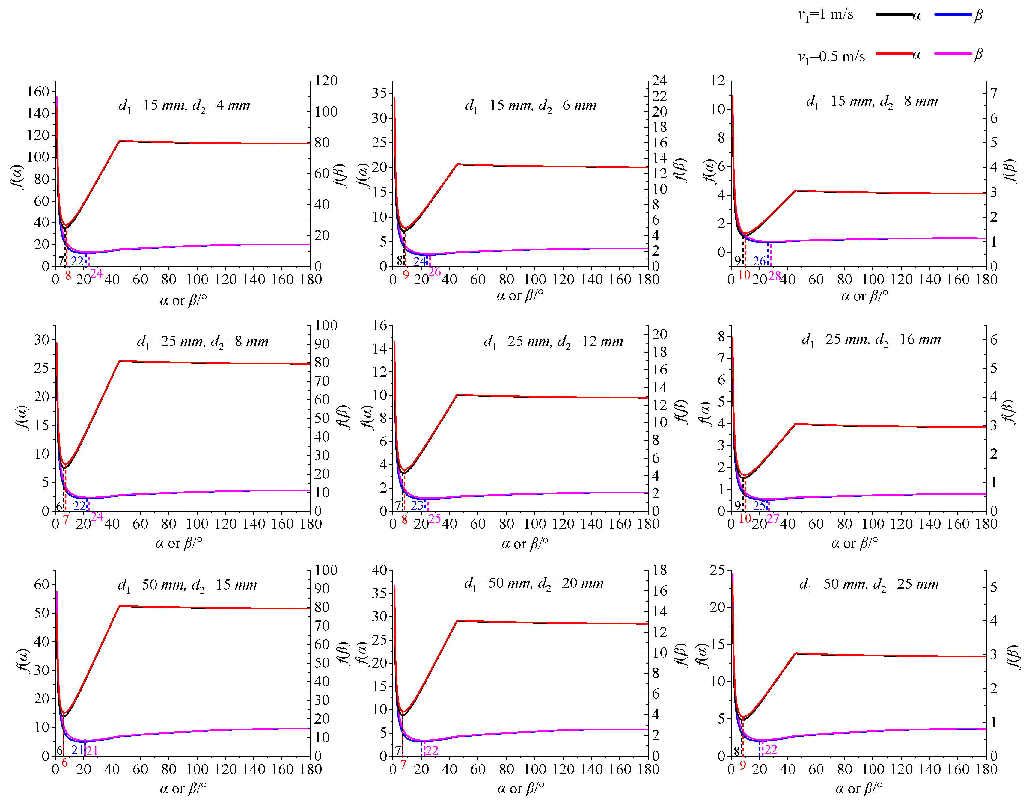
3.3.2. Optimal Reducing Angle and Expanding Angle

Following a consolidation of similar items in Equations (11)–(16), it was found that λr, λe, ξr, and ξe are functions of α and β. This led to the derivation of Equation (25). It was observed from Equation (25) that p2 decreased with the decreasing values of f(α) and f(β), resulting in p2 being at a minimum when both f(α) and f(β) reached their minimum, leading to maximum throat negative pressure.
p 2 = p 3 + 1 γ 4 + f ( β ) + 0.6 λ t f ( α ) + f ( β ) + 1.2 λ t Δ p ,
where
f ( α ) = 0.089 R e 1 0.25 tan α 2 ( γ 3.75 1 ) + 0.177 sin α 2 ( γ 4 γ 2 ) , α 45 ° 0.089 R e 1 0.25 tan α 2 ( γ 3.75 1 ) + 0.111 sin α 2 ( γ 4 γ 2 ) , 45 ° < α 180 ° f ( β ) = 0.058 R e 1 0.25 tan β 2 ( γ 3.75 1 ) + 1.209 sin β 2 ( γ 2 1 ) 2 , β 45 ° 0.058 R e 1 0.25 tan β 2 ( γ 3.75 1 ) + 0.465 ( γ 2 1 ) 2 , 45 ° < β 180 °
The extreme points varied with changes in the inlet velocity and the parameters of the Venturi injector. Therefore, the inlet velocity, as well as the inlet and throat diameters, were substituted into f(α) and f(β) to determine the optimal reducing angle and expanding angle. The structure parameters of the Venturi injector were chosen by referencing common products available in the market, as depicted in Figure 10. It was difficult to find the extreme points directly from the expressions of f(α) and f(β). Consequently, values of α and β were iterated at 1° intervals between 0° and 180° to identify the extreme points for Venturi injectors with different structural configurations. The corresponding relationship between α, β and f(α), f(β) was presented in Figure 10. There were significant differences on f(α) and f(β) when the inlet and throat diameter changed while the extreme points of α and β were close. It was observed that f(α) initially decreased and then increased as α increased. Similarly, from Figure 10, it was noted that f(β) initially decreased, followed by an increase, and then exhibited a slight decrease as β increased. Despite subtle variations in the values of f(α) and f(β) with changes in the inlet velocity, the optimal reducing and expanding angles only marginally increased with an increase in the inlet velocity. Significant differences were observed in f(α) and f(β) with changes in the inlet and throat diameters, despite the close proximity of the extreme points of α or β. The values of α and β that minimized f(α) and f(β) were found to be in the ranges of 20–28° and 6–10°, respectively. Additionally, minimal changes were observed in f(α) and f(β) when α and β varied near their extreme points.

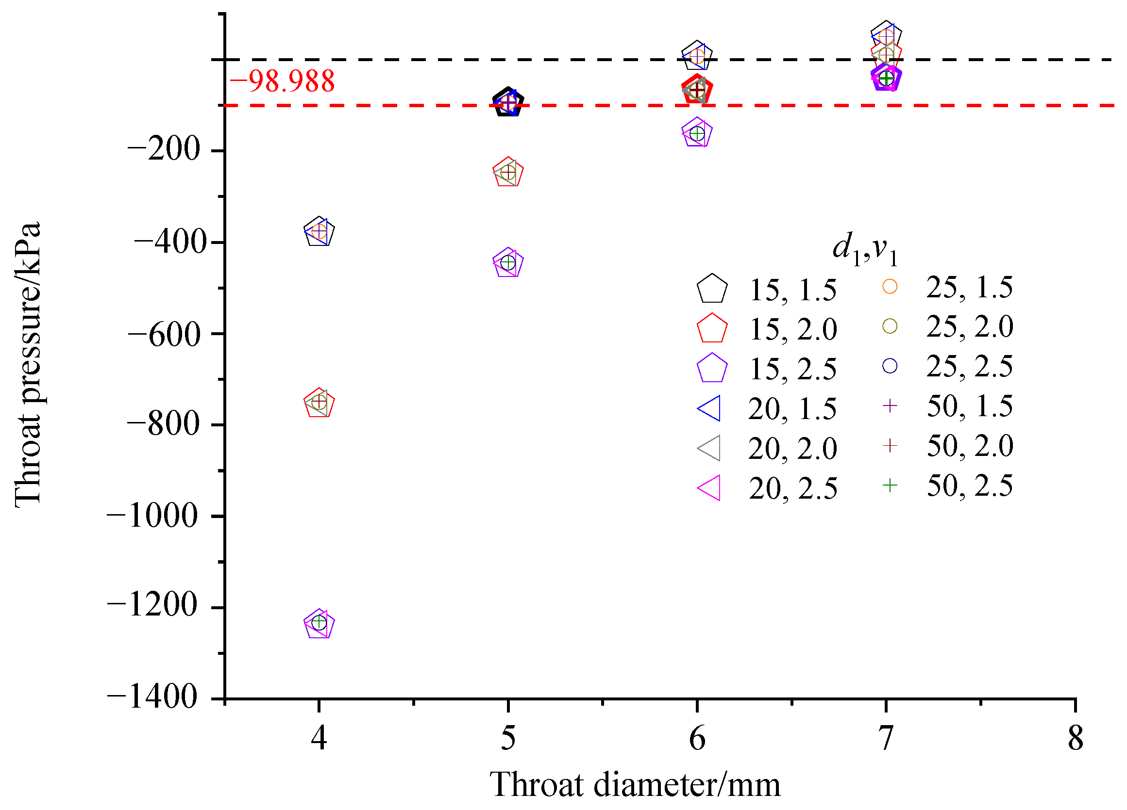
3.3.3. Optimal Throat Diameter

Equation (3) revealed that as the negative pressure within the Venturi throat increased, the suction flow rate also increased. In fact, the suction flow rate would remain unchanged if the negative pressure of the Venturi injector increased to a certain value. This was because the cavitation occurred in the Venturi throat when the negative pressure was high, and bubbles hindered the suction of the fertilizer. The optimization of throat negative pressure is achieved by increasing it to an appropriate level while avoiding cavitation. The saturated vapor pressure of water at room temperature (25 °C) was 2337 Pa, and the relative pressure was −98.988 kPa. Thus, cavitation would occur in the Venturi throat when the throat pressure was less than −98.988 kPa. The throat pressure should be better between −98.988 kPa and 0 kPa. The optimal range for the reducing and expanding angles was found to be 20–28° and 6–10°, respectively, with marginal differences in throat pressures within this range. In this study, the optimal throat diameter of the Venturi injector was explored based on a reducing angle of 24° and an expanding angle of 8°. The throat length equaled the inlet diameter. The inlet diameters (15, 20, 25, 30, and 50 mm) were chosen following common market products. To facilitate production, the throat diameter was rounded to a range of 5–8 mm, as diameters under 5 mm would be impractical for throat section production. The Venturi injector was typically utilized in drip irrigation, where the standard dripper working pressure was 100 kPa. Thus, for this investigation, the outlet pressure of the Venturi injector was set at 100 kPa. Common flow rates for drip irrigation systems range from 1.5 to 2.5 m3/h. Thus, flow rates of 1.5, 2.0, and 2.5 m3/h were employed in this study.
These parameters were input into Equation (24) to calculate the throat pressure, the results of which are presented in Figure 11. Interestingly, it was observed that little influence of the inlet diameter on the throat pressure. The negative pressure in the throat section increased as inlet flow rates increased and throat diameters decreased. For an inlet flow rate of 1.5 m3/h, the negative pressure within the throat section surpassed the cavitation threshold pressure when the throat diameter was less than 5 mm. Conversely, the throat pressure exceeded 0 when the throat diameter exceeded 6 mm. Consequently, the optimal throat diameter was determined to be 5 mm at an inlet flow rate of 1.5 m−3h. Similarly, at inlet flow rates of 2.0 and 2.5 m3/h, the optimal throat diameters were found to be 6 mm and 7 mm, respectively.

4. Discussion

The radial velocity gradient in the expanding section was observed to be greater than that in the reducing section. This disparity indicated that the expanding section of the Venturi tube would induce more significant interference with water flow, ultimately leading to a higher pressure loss compared to the reducing section. Notably, this study was conducted without considering cavitation, assuming that cavitation would occur when the throat pressure was less than −98.988 kPa. Similar findings were also reported by several researchers [31,32]. The optimal reducing and expanding angles of the Venturi injector were derived based on the formula for calculating throat pressure. Regarding the investigation of the optimal reducing and expanding angles, some researchers have explored this through experiments and numerical simulations. For instance, it was discovered that for a Venturi injector with an inlet diameter of 25 mm and a throat diameter of 5 mm operated under an inlet flow of 1 ms−1, the optimal reducing and expanding angles were found to be 20 and 8° [33]. Similarly, another study revealed that when the inlet flow was 0.519 ms−1, the inlet diameter was 15 mm, the throat diameter was 5 mm, and the optimal reducing and expanding angles were 25 and 7° [34].
By substituting the aforementioned data into Equation (26) and rounding α and β between 0 and 180° into f(α) and f(β), the obtained optimal reducing and expanding angles were consistent with the results of the aforementioned research. This reaffirmed the accuracy of the formula proposed in this study for calculating the throat pressure of the Venturi injector.

5. Conclusions

(1)
Frictional losses and local head losses in the reducing, throat, and expanding sections of the Venturi injector were analyzed based on fluid mechanics. Subsequently, a theoretical equation for calculating the head loss between the inlet and outlet of the Venturi tube was proposed. To verify and refine the theoretical equation, simulations based on CFD methods were conducted. The coefficient of determination of the regression equation was 0.945. The average deviation between the simulated and calculated head loss was 4.43%. The regression equation can be reliably utilized for head loss calculations in the Venturi tube;
(2)
The equation for calculating the throat pressure of the Venturi injector was derived based on the regression equation for head loss. Subsequently, the optimal structure parameters of the Venturi injector were analyzed to maximize the suction flow rate of the Venturi injector under identical inlet and outlet pressures. The optimal throat length and suction pipe diameter were set equal to the throat diameter of the Venturi injector. The optimal range for the reducing angle and expanding angle of the Venturi injector were identified as 20–28° and 6–10°, respectively. Moreover, it was determined that the optimal throat diameter fell within the range of 5–7 mm when the inlet flow rate ranged from 1.5 to 2.5 m3/h. These results provide a theoretical framework for parameter optimization in diverse applications;
(3)
The throat pressure calculation model established in this study has significant engineering application value. When certain parameters (such as inlet flow rate and inlet diameter) have been determined in actual working conditions, the optimal structural parameters can be rapidly solved based on this model. For open systems with completely variable parameters, an optimization range is provided that includes the contraction angle, diffusion angle, and throat diameter. The model’s versatility extends to a range of applications, including agricultural irrigation and fertilization and industrial liquid mixing, among others.

Author Contributions

Conceptualization, Z.Z. and P.T.; methodology, Y.L.; software, Z.Z.; validation, Z.Z. and Y.L.; resources, F.H.; data curation, Z.Z.; writing—original draft preparation, Z.Z.; writing—review and editing, Z.Z. and J.G.; funding acquisition, Z.Z. and J.G. All authors have read and agreed to the published version of the manuscript.

Funding

This research was funded by the Science and Technology Project of Jiangsu Vocational College of Agriculture and Forestry, grant number 2024rc44; Changzhou Science and Technology Support Program, grant number CJ20235054; “333 Project” of Jiangsu Province, grant number (2022)3-23-070; and The Key Research and Development Program of Jiangsu Province, grant number BE2021379.

Data Availability Statement

Since the dataset collected for this experiment is the public property of the laboratory, if you need the experimental dataset, please contact the corresponding author via email at zhangzhiyang@jsafc.edu.cn or zhangzhiyan94@163.com.

Acknowledgments

The authors are thankful to the editor and reviewers for their valuable comments in improving the quality of this paper.

Conflicts of Interest

Author Feng Huang was employed by the company Nanjing Wotian Intelligent Technology Company Limited. The remaining authors declare that the research was conducted in the absence of any commercial or financial relationships that could be construed as a potential conflict of interest.

Abbreviations

The following abbreviations are used in this manuscript:
CFDComputational Fluid Dynamics
Kswall roughness constant
R2coefficient of determination
ReReynolds number
SIMPLE Semi-Implicit Method for Pressure-Linked Equations
Y+wall-distance non-dimensional parameter

References

  1. Li, P.; Li, H.; Li, J.; Huang, X.Q.; Liu, Y.; Jiang, Y. Effect of Aeration on Blockage Regularity and Microbial Diversity of Blockage Substance in Drip Irrigation Emitter. Agriculture 2022, 12, 1941. [Google Scholar] [CrossRef]
  2. Li, J.; Meng, Y.; Liu, Y. Hydraulic performance of differential pressure tanks for fertigation. Trans. ASAE 2006, 49, 1815–1822. [Google Scholar]
  3. Li, H.; Li, H.; Huang, X.; Han, Q.; Yuan, Y.; Qi, B. Numerical and Experimental Study on the Internal Flow of the Venturi Injector. Process 2020, 8, 64. [Google Scholar]
  4. Sobenko, L.R.; Frizzone, J.A.; Camargo, A.P.D.; Saretta, E.; Rocha, H.S.D. Characterization of venturi injector using dimensional analysis characterization of venturi injector using dimensional analysis. Rev. Bras. Eng. Agrícola Ambient. 2019, 23, 484–491. [Google Scholar] [CrossRef]
  5. Fan, J.; Wu, L.; Zhang, F.; Yan, S.; Xiang, Y. Evaluation of drip fertigation uniformity affected by injector type, pressure difference and lateral layout. Irrig. Drain. 2017, 66, 520–529. [Google Scholar]
  6. Li, J.; Meng, Y.; Li, B. Field evaluation of fertigation uniformity as affected by injector type and manufacturing variability of emitters. Irrig. Sci. 2007, 25, 117–125. [Google Scholar] [CrossRef]
  7. Yuan, Z.; Choi, C.Y.; Waller, P.M.; Colaizzi, P. Effects of liquid temperature and viscosity on venturi injectors. Trans. ASAE 2000, 43, 1441–1447. [Google Scholar]
  8. Neto, I.E.L.; Porto, R.D.M. Performance of low–cost ejectors. J. Irrig. Drain. Eng. 2004, 130, 122–128. [Google Scholar]
  9. Hu, G.; Guan, X.; Li, S.; Liu, N.; Zhang, J.; Zhang, J.; Wang, Z. Structure optimization and fertilizer injection performance analysis of a non–axisymmetric Venturi injector. Irrig. Drain. 2023, 73, 400–414. [Google Scholar] [CrossRef]
  10. Bartzanas, T.; Kacira, M.; Zhu, H.; Karmakar, S.; Tamimi, E.; Katsoulas, N.; Lee, I.B.; Kittas, C. Computational fluid dynamics applications to improve crop production systems. Comput. Electron. Agric. 2013, 93, 151–167. [Google Scholar]
  11. Dione, F.; Cong, T.; Jayeola, M. Open-FOAM CFD simulation of critical heat flux in vertical pipe under typically PWR conditions. Ann. Nucl. Energy 2022, 174, 109174. [Google Scholar] [CrossRef]
  12. Huang, X.; Li, G.; Wang, M. CFD simulation to the flow field of venturi injector. In Computer and Computing Technologies in Agriculture II, Volume 2: Proceedings of the Second IFIP International Conference on Computer and Computing Technologies in Agriculture (CCTA2008), 18–20 October 2008, Beijing, China; Li, D., Zhao, C., Eds.; Springer: New York, NY, USA, 2009; pp. 805–815. [Google Scholar]
  13. Wang, H.; Wang, J.; Yang, B.; Mo, Y.; Zhang, Y.; Ma, X. Simulation and optimization of venturi injector by machine learning algorithms. J. Irrig. Drain. Eng. 2020, 146, 04020021. [Google Scholar]
  14. Zhang, L.; Wei, Z.; Qian, Z. Structural optimization of the low-pressure venturi injector with double suction ports based on computational fluid dynamics and orthogonal test. Desalin. Water Treat. 2021, 214, 347–354. [Google Scholar]
  15. Liu, J.P.; Hussain, Z.; Wang, X.J.; Li, Y.F. Optimization and Numerical Simulation of the Internal Flow Field of Water–Pesticide Integrated Microsprinklers. Irrig. Drain. 2023, 72, 328–342. [Google Scholar]
  16. Chen, A.; Yu, Y. CFD-DEM simulation on the complex gas–solid flow in a closed chamber with particle groups. J. Mech. Sci. Technol. 2022, 36, 5523–5535. [Google Scholar]
  17. Im, K.; Kim, H.; Lai, M.; Tacina, R. Parametric study of the swirler/venturi spray injectors. J. Propuls. Power 2001, 17, 717–727. [Google Scholar]
  18. Manzano, J.; De Azevedo, B.M.; Do Bomfim, G.V.; Royuela, Á.; Palau, C.V.; De, A.; Viana, T.V. Design and prediction performance of Venturi injectors in drip irrigation. Rev. Bras. Eng. Agric. Ambient. 2014, 18, 1209–1217. [Google Scholar]
  19. Manzano, J.; Palau, C.; de Azevedo, B.; do Bomfim, G.; Vasconcelos, D. Characterization and selection method of Venturi injectors for pressurized irrigation. Rev. Cienc. Agron. 2018, 49, 201–210. [Google Scholar]
  20. Chen, L.; Sun, Z.; Ma, H.; Gao, K.; Ma, G.; Deng, Y. Structural parameters of venturi injector for periodic air recovery based on response surface methodology. Chem. Eng. Process. Intensif. 2023, 193, 109551. [Google Scholar]
  21. Valiantzas, J.D. Explicit power formula for the darcy–weisbach pipe flow Equation: Application in optimal pipeline design. J. Irrig. Drain. Eng. 2008, 134, 454–461. [Google Scholar] [CrossRef]
  22. Marui–Paloka, E.; Paanin, I. Effects of boundary roughness and inertia on the fluid flow through a corrugated pipe and the formula for the darcy–weisbach friction coefficient. Int. J. Eng. Sci. 2020, 152, 103293. [Google Scholar]
  23. Rettore Neto, O.; de Miranda, J.H.; Frizzone, J.A.; Workman, S.R. Local Head Loss of Non–Coaxial Emitters Inserted in Polyethylene Pipe. Trans. ASABE 2009, 52, 729–738. [Google Scholar]
  24. José, H.N.F.; Faria, L.C.; Neto, O.R.; Diotto, A.V.; Colombo, A. Methodology for determining the emitter local head loss in drip irrigation systems. J. Irrig. Drain. Eng. 2021, 147, 06020014. [Google Scholar]
  25. Xu, F. Influence of Valve on Flow Resistance of Piping System. China Nucl. Power 2017, 10, 64–68. [Google Scholar]
  26. Jiang, Y.; Li, H.; Xiang, Q.; Chen, C. Comparison of PIV Experiment and Numerical Simulation on the Velocity Distribution of Intermediate Pressure Jets with Different Nozzle Parameters. Irrig. Drain. 2017, 66, 510–519. [Google Scholar]
  27. Tang, P.; Juárez, J.M.; Li, H. Investigation on the effect of structural parameters on cavitation characteristics for the venturi tube using the CFD method. Water 2019, 11, 2194. [Google Scholar] [CrossRef]
  28. Hu, X.; Chen, X. Optimisation of fertiliser dissolution under differential pressure tank during fertigation. Biosyst. Eng. 2021, 206, 79–93. [Google Scholar]
  29. Dong, C.; Zhu, J.; Miller, C.F. Evaluation of six aerator modules built on venturi air injectors using clean water test. Water Sci. Technol. 2009, 60, 1353–1359. [Google Scholar]
  30. Mukesh, K.; Rajput, T.B.S.; Neelam, P. Effect of system pressure and solute concentration on fertilizer injection rate of a venturi for fertigation. J. Agric. Eng. 2012, 49, 9–13. [Google Scholar] [CrossRef]
  31. Xu, Y.; Chen, Y.; Wang, Z.; Zhou, L.; Yan, H. Investigation of the cavitation fluctuation characteristics in a Venturi injector. Fluid Dyn. Res. 2015, 47, 025506. [Google Scholar]
  32. Simpson, A.; Ranade, V.V. Modeling hydrodynamic cavitation in venturi: Influence of venturi configuration on inception and extent of cavitation. AIChE J. 2019, 65, 421–433. [Google Scholar] [CrossRef]
  33. Liu, Y.; Shen, M.; Jiang, X.; Jiang, K.; Feng, Q. Structure Optimization of Suction Device and Performance Test of Integrated Water and Fertilizer Fertigation Machine. Trans. Chin. Soc. Agric. Mach. 2015, 11, 76–81+48. [Google Scholar]
  34. Qiu, Z.; Bao, A. Numerical Study on Concentration Affected by Structure Parameters—Based on Parallel Venturi Fertilizer Applicator. J. Agric. Mechan. Res. 2012, 4, 42–45. [Google Scholar]
Figure 1. Structure diagram of the Venturi injector.
Fluids 10 00087 g001
Figure 2. Structure diagram of the Venturi tube.
Fluids 10 00087 g002
Figure 3. Reducing section of Venturi tube.
Fluids 10 00087 g003
Figure 4. Mesh generation of the Venturi tube.
Fluids 10 00087 g004
Figure 5. Distribution of static pressure in the axial direction of the Venturi tube.
Fluids 10 00087 g005
Figure 6. The prototype of the Venturi tube.
Fluids 10 00087 g006
Figure 7. Arrangement for Evaluating the Hydraulic Performance of the Venturi Tube. 1. Motor 2. Pump 3. Electromagnetic flowmeter 4. Valve 5. Digital pressure gauge 6. Venturi tube 7. Digital pressure gauge 8. Valve 9. Water tank.
Fluids 10 00087 g007
Figure 8. Velocity contours of the flow field in the Venturi tube.
Fluids 10 00087 g008
Figure 9. Pressure contours of the flow field in the Venturi tube.
Fluids 10 00087 g009
Figure 10. Corresponding relationship between α, β and f(α), f(β) in different conditions.
Fluids 10 00087 g010
Figure 11. Throat pressure of the Venturi injector with different inlet and throat diameters.
Fluids 10 00087 g011
Table 1. Optimal structural parameters of the Venturi fertilizer under different conditions.
AuthorSpecific Operating ConditionsOptimal Structural Parameters of the Venturi Fertilizer Applicator
Huang et al. [12]A 3-factor 3-level full factor experimentThroat diameter of 8 mm, Slot diameter of 18.5 mm, Throat length of 14 mm
Wang et al. [13]Inlet diameter of 14 mm, Throat diameter of 15 mm, Inlet pressure of 0.3 MPa, Outlet pressure of 0.1 MPaContraction angle of 20–30°, Diffusion angle of 8–10°, Throat length of 40–50 mm, Ratio of throat diameter to nozzle diameter of 1.5–1.66
Zhang et al. [14]An orthogonal test of six factors and five levelsConvergence angle of 24°, Throat contraction ratio of 0.2, Throat length-diameter ratio of 2.0, Expanding angle of 6°
Table 2. Orthogonal design of the Venturi tube experiment.
FactorLevel
Reducing angle (°)10, 20, 30, 40, 50
Expanding angle (°)10, 20, 30, 40, 50
Inlet diameter (mm)15, 20, 25, 30, 50
Throat diameter (mm)5, 6, 7, 8, 9
Inlet flow velocity (m/s)1, 1.2, 1.4, 1.6, 1.8
Table 3. Comparison of the inlet pressure for the Venturi tube in experimental and simulation results.
Inlet Flow (m3/h)Outlet Pressure (kPa)Inlet Pressure
Experiment
(kPa)
Simulation (kPa)Deviation
Rs = 0.3Rs = 0.4Rs = 0.5
1019.8 ± 0.520.720.420.22.02%~4.55%
15067.2 ± 0.670.770.470.24.46%~5.21%
1100115.5 ± 0.5120.7120.4120.24.06%~4.50%
1150162.4 ± 0.2170.7170.4170.24.80%~5.11%
Table 4. Calculation and simulation head losses of the Venturi tube at different flow rates.
Velocity (m/s)Simulation Loss (m)Calculation Loss (m)Deviation (%)
10.9121.60243.07
1.21.2822.28762.73
1.41.7073.09286.45
1.62.1884.015114.04
1.82.7245.056145.57
Table 5. Loss of Venturi tubes with different structures.
α
(°)
β
(°)
d1
(mm)
d2
(mm)
v1
(m/s)
hs1
(m)
h1
(m)
hs2
(m)
h2
(m)
hs3
(m)
h3
(m)
hs
(m)
h1–3
(m)
δ
(%)
101015510.330.340.210.220.520.531.061.092.26
20201561.20.180.170.110.120.490.490.780.780.00
30301571.40.120.120.090.080.430.430.630.630.00
40401581.60.070.090.040.050.350.360.460.508.68
50501591.80.070.070.040.040.240.250.350.362.71
20302051.61.851.851.361.349.809.7813.0312.970.49
30402061.81.181.210.650.697.187.229.029.131.19
405020710.230.230.120.121.241.251.591.600.81
50102081.20.220.210.100.090.240.240.550.533.24
10202091.40.170.180.060.070.400.420.630.676.44
30502551.22.832.791.801.7720.2820.1824.9224.750.71
40102561.41.932.090.930.982.853.075.716.137.35
50202571.61.621.610.660.594.053.926.336.133.16
10302581.81.091.030.450.394.624.516.165.933.80
204025910.140.170.080.080.961.011.181.267.48
40203051.814.6414.786.666.8242.1343.9563.4365.553.35
503030612.392.510.961.038.889.4012.2312.935.74
10403071.21.371.630.590.689.549.9911.5012.306.90
20503081.41.041.060.410.477.668.269.119.797.52
30103091.60.870.940.340.341.461.582.672.867.09
50405051.473.5577.723.2226.27382.35409.59479.12513.567.19
10505061.625.7431.9412.6513.96286.13299.18324.52345.086.33
20105071.818.5920.67.638.2545.3248.671.5477.448.25
302050814.254.561.441.5615.3416.2321.0322.366.33
40305091.24.634.801.161.2320.4420.9726.2327.002.95
α, β, d1, d2, v1, and δ denote the reducing angle, expanding angle, inlet diameter, throat diameter, inlet velocity, and deviation between hs and h1–3. hs1, hs2, hs3, and hs are the simulation head loss in the reducing section, throat section, expanding section, and between the inlet and outlet. h1, h2, h3, and h1–3 are head loss in the reducing section, throat section, expanding section, and between the inlet and outlet calculated by regression Equation.
Table 6. Verification of the modified formula’s accuracy outside the orthogonal test’s value range.
α (°)β (°)d1 (mm)d2 (mm)v1 (m/s)hs (m)h1–3 (m)Deviation (%)
60180151010.130.126.71
80160201121.621.545.13
9014025122.23.963.696.75
10012025132.42.812.733.00
12010030142.65.575.128.11
1409030152.42.992.922.34
160805016215.7715.442.06
1806050171.88.217.903.72
Disclaimer/Publisher’s Note: The statements, opinions and data contained in all publications are solely those of the individual author(s) and contributor(s) and not of MDPI and/or the editor(s). MDPI and/or the editor(s) disclaim responsibility for any injury to people or property resulting from any ideas, methods, instructions or products referred to in the content.

