On the Kutta Condition in Compressible Flow over Isolated Airfoils

Abstract

This paper presents a novel and accurate method to implement the Kutta condition in solving subsonic (subcritical) inviscid isentropic compressible flow over isolated airfoils using the stream function equation. The proposed method relies on body-fitted grid generation and solving the stream function equation for compressible flows in computational domain using finite-difference method. An expression is derived for implementing the Kutta condition for the airfoils with both finite angles and cusped trailing edges. A comparison of the results obtained from the proposed numerical method and the results from experimental and other numerical methods reveals that they are in excellent agreement, which confirms the accuracy and correctness of the proposed method.

1. Introduction

Nowadays, computational fluid dynamics complements its experimental and theoretical counterpart. Benefiting from high-speed digital computers, the use of sophisticated numerical methods has made possible the numerical solution of fluid flow problems which were heretofore intractable. Compressible flows over airfoils and wings play a vital role in computational aerodynamics, and demand advanced computational techniques. Since introducing the source and vortex panel methods in the late 1960s [1], they have become the standard tools to numerically solve low-speed flows over bodies of arbitrary shape, and have had extensive applications in flow modeling [2,3,4,5,6]. The panel methods used for the simulation of flows over an airfoil are concerned with the vortex panel strength and circulation quantities; the evaluation of such quantities allows one to calculate the velocity distribution over the airfoil surface, and hence, to determine the pressure coefficients. The Kutta condition (a viscous boundary condition based on physical observation used with inviscid theoretical model) states that the flow leaves the sharp trailing edge of an airfoil smoothly [7]. Various methods have been proposed to impose the Kutta condition [8,9,10]. In panel methods, the Kutta condition is incorporated in the numerical formulation by requiring that the strength of vortex sheet is zero at the airfoil trailing edge. Moreover, the use of panel methods along with the compressibility corrections such as the Prandtl-Glauert method [11] allow one to consider the compressible flows over bodies. The panel methods have been extensively investigated in the aerodynamics literature, so these will not be discussed further here. However, these methods often have trouble with accuracy at the trailing edge of airfoils with zero angle cusped trailing edges [12]. Moreover, the compressibility corrections do not give accurate results for the compressible flows over airfoils of any shape at any angle of attack. For example, the Prandtl-Glauert method is based on the linearized perturbation velocity potential equation, and hence, it is limited to thin airfoils at small angles of attack [4].

In this paper, we propose a novel method to numerically solve the steady irrotational compressible flow over an airfoil which is exempt from considerations of quantities such as the vortex panel strength and circulation. This method takes advantage of an O-grid, generated by the elliptic grid generation technique, over the flow field and approximates the flow field quantities such as stream function, density, velocity, pressure, speed of sound, and Mach number at the nodal points. An accurate Kutta condition scheme is proposed and implemented into the computational loop by an exact derived expression for the stream function. The exact expression is general and encompasses both the finite-angle and cusped trailing edges. Finally, the results obtained from the proposed numerical method, and the results from experimental and other numerical methods, are compared to reveal the accuracy of the proposed method (The material given in this article are implemented in the code FOILcom which is freely available at: DOI:10.13140/RG.2.2.36459.64801/1).

It is worth emphasizing that the stream function equation considered in this study is completely equivalent to the full potential equation. Here, the stream function equation is solved in non-conservative form and can be employed to obtain accurate results for subsonic (subcritical) inviscid isentropic compressible flow over isolated airfoils. The conservative stream function equation, along with upwinding schemes such as artificial compressibility [13], can be used to solve transonic flows over airfoils which is not considered in this study.

2. Governing Equations

The stream function equation for two-dimensional, irrotational, steady, and isentropic flow of a compressible fluid in non-conservative form is as follows [14,15,16]

$$(c^2-u^2){\psi }_{xx}+(c^2-v^2){\psi }_{yy}-2uv{\psi }_{xy}=0$$

(1)

where $\psi$ is the stream function, $u$ and $v$ are the components of the velocity vector $\mathbf{V}$, i.e.,$\mathbf{V}=u\mathbf{i}+v\mathbf{j}$ ($\mathbf{i}$ and $\mathbf{j}$ are the unit vectors in $x$ and $y$ directions, respectively). For a two-dimensional compressible flow,

$$u=\frac{{\rho }_0}{\rho }{\psi }_y$$

(2)

$$v=-\frac{{\rho }_0}{\rho }{\psi }_x$$

(3)

$c$ is the local sound speed [4]

$$c^2=c_0^2-\frac{\gamma -1}{2}{V}^2=c_0^2-\frac{\gamma -1}{2}(u^2+v^2)$$

(4)

$c_0$ is the stagnation speed of sound, $\rho$ is the density, ${\rho }_0$ is the stagnation density, and $\gamma =c_p/c_v$ ($c_v$ and $c_p$ are the specific heats at constant volume and constant pressure, respectively) is the ratio of specific heats of gas (for air at standard conditions, $\gamma =1.4$). Dividing both sides of Equation (1) by $c^2$ and then substituting the expressions in Equations (2) and (3) into Equation (1) gives the stream function equation as

$$[1-\frac{1}{c^2}{(\frac{{\rho }_0}{\rho })}^2{\psi }_y^2]{\psi }_{xx}+[1-\frac{1}{c^2}{(\frac{{\rho }_0}{\rho })}^2{\psi }_x^2]{\psi }_{yy}+\frac{2}{c^2}{(\frac{{\rho }_0}{\rho })}^2{\psi }_x{\psi }_y{\psi }_{xy}=0$$

(5)

by substituting Equation (4) into Equation (5), we get

$$\begin{gathered} [1-\frac{1}{c_0^2-\frac{\gamma -1}{2}{(\frac{{\rho }_0}{\rho })}^2({\psi }_x^2+{\psi }_y^2)}{(\frac{{\rho }_0}{\rho })}^2{\psi }_y^2]{\psi }_{xx}+[1-\frac{1}{c_0^2-\frac{\gamma -1}{2}{(\frac{{\rho }_0}{\rho })}^2({\psi }_x^2+{\psi }_y^2)}{(\frac{{\rho }_0}{\rho })}^2{\psi }_x^2]{\psi }_{yy}+ \\ \frac{2}{c_0^2-\frac{\gamma -1}{2}{(\frac{{\rho }_0}{\rho })}^2({\psi }_x^2+{\psi }_y^2)}{(\frac{{\rho }_0}{\rho })}^2{\psi }_x{\psi }_y{\psi }_{xy}=0 \end{gathered}$$

(6)

and from the local isentropic stagnation properties of an ideal gas, we have

$$\frac{{\rho }_0}{\rho }={(1+\frac{\gamma -1}{2}{M}^2)}^{\frac{1}{\gamma -1}}={(1+\frac{\gamma -1}{2}\frac{u^2+v^2}{c^2})}^{\frac{1}{\gamma -1}}$$

(7)

$M=\frac{V}{c}$ is the local Mach number. Equations (6) and (7) should be solved simultaneously to obtain the local values of $\psi$ and $\rho$ in the flow field.

2.1. Transformation

The solution of the governing PDE is based on transformation of the physical domain $(x,y)$ and the governing equations into the regular computational domain $(\xi ,\eta )$ (see Figure 1). Therefore, the derivatives such as ${\psi }_x$, ${\psi }_y$, ${\psi }_{xx}$, ${\psi }_{yy}$, and ${\psi }_{xy}$ in the stream function equation, Equation (1), should be transformed from the physical domain $(x,y)$ to the computational domain $(\xi ,\eta )$ [17,18,19]. This transformation can be stated as

$$\xi \equiv \xi (x,y)$$

(8)

$$\eta \equiv \eta (x,y)$$

(9)

and the inverse transformation is given as below.

$$x\equiv x(\xi ,\eta )$$

(10)

$$y\equiv y(\xi ,\eta )$$

(11)

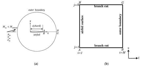
Figure 1. The physical and the computational domains. (a) Physical domain. (b) Computational domain.

Since the stream function equation involves first and second derivatives, relationships are needed to transform such derivatives from the $(x,y)$ system to the $(\xi ,\eta )$ one. In order to do this, the Jacobian of the transformation is needed, which is given below

$$2\mathrm{D}:J=J(\frac{x,y}{\xi ,\eta })=\left|\begin{array}{cc}{x}_{\xi }& y_{\xi }\\ x_{\eta }& y_{\eta }\end{array}\right|=x_{\xi }{y}_{\eta }-x_{\eta }{y}_{\xi }\ne 0$$

(12)

As will be shown, the transformation relations involve the Jacobian in denominator. Hence, it cannot be zero. Since we deal with the stream function equation, it is necessary to find relationships for the transformation of the first and second derivatives of the variable $\psi$ with respect to the variables $x$ and $y$. By using the chain rule, it can be concluded that

$$\frac{\partial \psi }{\partial x}=\frac{\partial \psi }{\partial \xi }\frac{\partial \xi }{\partial x}+\frac{\partial \psi }{\partial \eta }\frac{\partial \eta }{\partial x}=\frac{\partial \psi }{\partial \xi }{\xi }_x+\frac{\partial \psi }{\partial \eta }{\eta }_x$$

(13)

$$\frac{\partial \psi }{\partial y}=\frac{\partial \psi }{\partial \xi }\frac{\partial \xi }{\partial y}+\frac{\partial \psi }{\partial \eta }\frac{\partial \eta }{\partial y}=\frac{\partial \psi }{\partial \xi }{\xi }_y+\frac{\partial \psi }{\partial \eta }{\eta }_y$$

(14)

By interchanging $x$ and $\xi$, and $y$ and $\eta$, the following relationships can also be derived

$$\frac{\partial \psi }{\partial \xi }=\frac{\partial \psi }{\partial x}\frac{\partial x}{\partial \xi }+\frac{\partial \psi }{\partial y}\frac{\partial y}{\partial \xi }=\frac{\partial \psi }{\partial x}{x}_{\xi }+\frac{\partial \psi }{\partial y}{y}_{\xi }$$

(15)

$$\frac{\partial \psi }{\partial \eta }=\frac{\partial \psi }{\partial x}\frac{\partial x}{\partial \eta }+\frac{\partial \psi }{\partial y}\frac{\partial y}{\partial \eta }=\frac{\partial \psi }{\partial x}{x}_{\eta }+\frac{\partial \psi }{\partial y}{y}_{\eta }$$

(16)

By solving Equations (15) and (16) for $\frac{\partial \psi }{\partial x}$ and $\frac{\partial \psi }{\partial y}$, we finally obtain

$$\frac{\partial \psi }{\partial x}=\frac{1}{J}(y_{\eta }\frac{\partial \psi }{\partial \xi }-y_{\xi }\frac{\partial \psi }{\partial \eta })$$

(17)

$$\frac{\partial \psi }{\partial y}=\frac{1}{J}(-x_{\eta }\frac{\partial \psi }{\partial \xi }+x_{\xi }\frac{\partial \psi }{\partial \eta })$$

(18)

where $J=x_{\xi }{y}_{\eta }-x_{\eta }{y}_{\xi }$ is Jacobian of the transformation. By comparing Equations (13) and (17), and (14) and (18), it can be shown that

$${\xi }_x=\frac{1}{J}{y}_{\eta },{\xi }_y=-\frac{1}{J}{x}_{\eta }$$

(19)

$${\eta }_x=-\frac{1}{J}{y}_{\xi },{\eta }_y=\frac{1}{J}{x}_{\xi }$$

(20)

To transform terms in the stream function equation (Equation (6)), the second order derivatives are needed. Therefore,

$${\psi }_{xx}={({\psi }_x)}_x={(\frac{1}{J}(y_{\eta }{\psi }_{\xi }-y_{\xi }{\psi }_{\eta }))}_x$$

(21)

$${\psi }_{yy}={({\psi }_y)}_y={(\frac{1}{J}(-x_{\eta }{\psi }_{\xi }+x_{\xi }{\psi }_{\eta }))}_y$$

(22)

$${\psi }_{xy}={({\psi }_x)}_y={(\frac{1}{J}(y_{\eta }{\psi }_{\xi }-y_{\xi }{\psi }_{\eta }))}_y$$

(23)

which result in the following expressions for the second order derivatives

$$\begin{gathered} {\psi }_{xx}=\frac{(y_{\eta }^2{\psi }_{\xi \xi }-2y_{\xi }{y}_{\eta }{\psi }_{\xi \eta }+y_{\xi }^2{\psi }_{\eta \eta })}{J^2}+\frac{(y_{\eta }^2{y}_{\xi \xi }-2y_{\xi }{y}_{\eta }{y}_{\xi \eta }+y_{\xi }^2{y}_{\eta \eta })(x_{\eta }{\psi }_{\xi }-x_{\xi }{\psi }_{\eta })}{J^3}+ \\ \frac{(y_{\eta }^2{x}_{\xi \xi }-2y_{\xi }{y}_{\eta }{x}_{\xi \eta }+y_{\xi }^2{x}_{\eta \eta })(y_{\xi }{\psi }_{\eta }-y_{\eta }{\psi }_{\xi })}{J^3} \end{gathered}$$

(24)

$$\begin{gathered} {\psi }_{yy}=\frac{(x_{\eta }^2{\psi }_{\xi \xi }-2x_{\xi }{x}_{\eta }{\psi }_{\xi \eta }+x_{\xi }^2{\psi }_{\eta \eta })}{J^2}+\frac{(x_{\eta }^2{y}_{\xi \xi }-2x_{\xi }{x}_{\eta }{y}_{\xi \eta }+x_{\xi }^2{y}_{\eta \eta })(x_{\eta }{\psi }_{\xi }-x_{\xi }{\psi }_{\eta })}{J^3}+ \\ \frac{(x_{\eta }^2{x}_{\xi \xi }-2x_{\xi }{x}_{\eta }{x}_{\xi \eta }+x_{\xi }^2{x}_{\eta \eta })(y_{\xi }{\psi }_{\eta }-y_{\eta }{\psi }_{\xi })}{J^3} \end{gathered}$$

(25)

$$\begin{gathered} {\psi }_{xy}=\frac{1}{J}[-x_{\eta }(\frac{y_{\xi \eta }{\psi }_{\xi }+y_{\eta }{\psi }_{\xi \xi }-y_{\xi \xi }{\psi }_{\eta }-y_{\xi }{\psi }_{\xi \eta }}{J}-\frac{(y_{\eta }{\psi }_{\xi }-y_{\xi }{\psi }_{\eta })(x_{\xi \xi }{y}_{\eta }+x_{\xi }{y}_{\xi \eta }-x_{\xi \eta }{y}_{\xi }-x_{\eta }{y}_{\xi \xi })}{J^2})+ \\ {x}_{\xi }(\frac{y_{\eta \eta }{\psi }_{\xi }+y_{\eta }{\psi }_{\xi \eta }-y_{\xi \eta }{\psi }_{\eta }-y_{\xi }{\psi }_{\eta \eta }}{J}-\frac{(y_{\eta }{\psi }_{\xi }-y_{\xi }{\psi }_{\eta })(x_{\xi \eta }{y}_{\eta }+x_{\xi }{y}_{\eta \eta }-x_{\eta \eta }{y}_{\xi }-x_{\eta }{y}_{\xi \eta })}{J^2})] \end{gathered}$$

(26)

The finite-difference method can be used to discretize the above expressions in the regular computational domain $(\xi ,\eta )$. The actual values of $\xi$ and $\eta$ in the computational domain are immaterial, because they do not appear in the final expressions. Thus, without a loss of generality, we can select the coordinates of the node $A$ in the computational domain as $\xi =\eta =1$ and the mesh size as $\mathsf{\Delta }\xi =\mathsf{\Delta }\eta =1$ [19]. Therefore, we have [17]

$${(f_{\xi })}_{i,j}=\frac{1}{2}(f_{i+1,j}-f_{i-1,j})$$

(27)

$${(f_{\eta })}_{i,j}=\frac{1}{2}(f_{i,j+1}-f_{i,j-1})$$

(28)

$${(f_{\xi \xi })}_{i,j}=(f_{i+1,j}-2f_{i,j}+f_{i-1,j})$$

(29)

$${(f_{\eta \eta })}_{i,j}=(f_{i,j+1}-2f_{i,j}+f_{i,j-1})$$

(30)

$${(f_{\xi \eta })}_{i,j}=\frac{1}{4}(f_{i+1,j+1}-f_{i-1,j+1}-f_{i+1,j-1}+f_{i-1,j-1})$$

(31)

where $f\equiv x,y,\psi$.

2.2. Boundary Conditions

Conditions at infinity: Far away from the airfoil surface (toward infinity), in all directions, the flow approaches the free stream conditions. The known free stream conditions are the velocity $V_{\infty }$, the pressure $p_{\infty }$, the density ${\rho }_{\infty }$, and the temperature $T_{\infty }$. Thus, the free stream Mach number is

$$M_{\infty }=\frac{V_{\infty }}{c_{\infty }}<M_{\mathrm{critical}}$$

(32)

and the speed of sound $c_{\infty }$ is

$$c_{\infty }=\sqrt{\gamma R{T}_{\infty }}$$

(33)

where $R$ is the specific gas constant, which is a different value for different gases. For air at standard conditions, $R_{\mathrm{air}}=287\mathrm{J}/(\mathrm{kg}.\mathrm{K})$, ${\gamma }_{\mathrm{air}}=1.4$, ${\rho }_{\infty }=1.23\mathrm{kg}/{\mathrm{m}}^3$, and $p_{\infty }=1.01\times {10}^5{ \mathrm{N}/\mathrm{m}}^2$. The critical Mach number $M_{\mathrm{critical}}$ is that free stream Mach number at which sonic flow is first achieved on the airfoil surface.

Condition on the airfoil surface: The relevant boundary condition at the airfoil surface for the inviscid flow is the no-penetration boundary condition. Thus, the velocity vector must be tangential to the surface. This wall boundary condition can be expressed by

$$\frac{\partial \psi }{\partial s}=0\hspace{1em}\hspace{1em}\mathrm{or}\hspace{1em}\psi =\mathrm{constant}$$

(34)

where $s$ is tangent to the surface.

2.3. Grid Generation

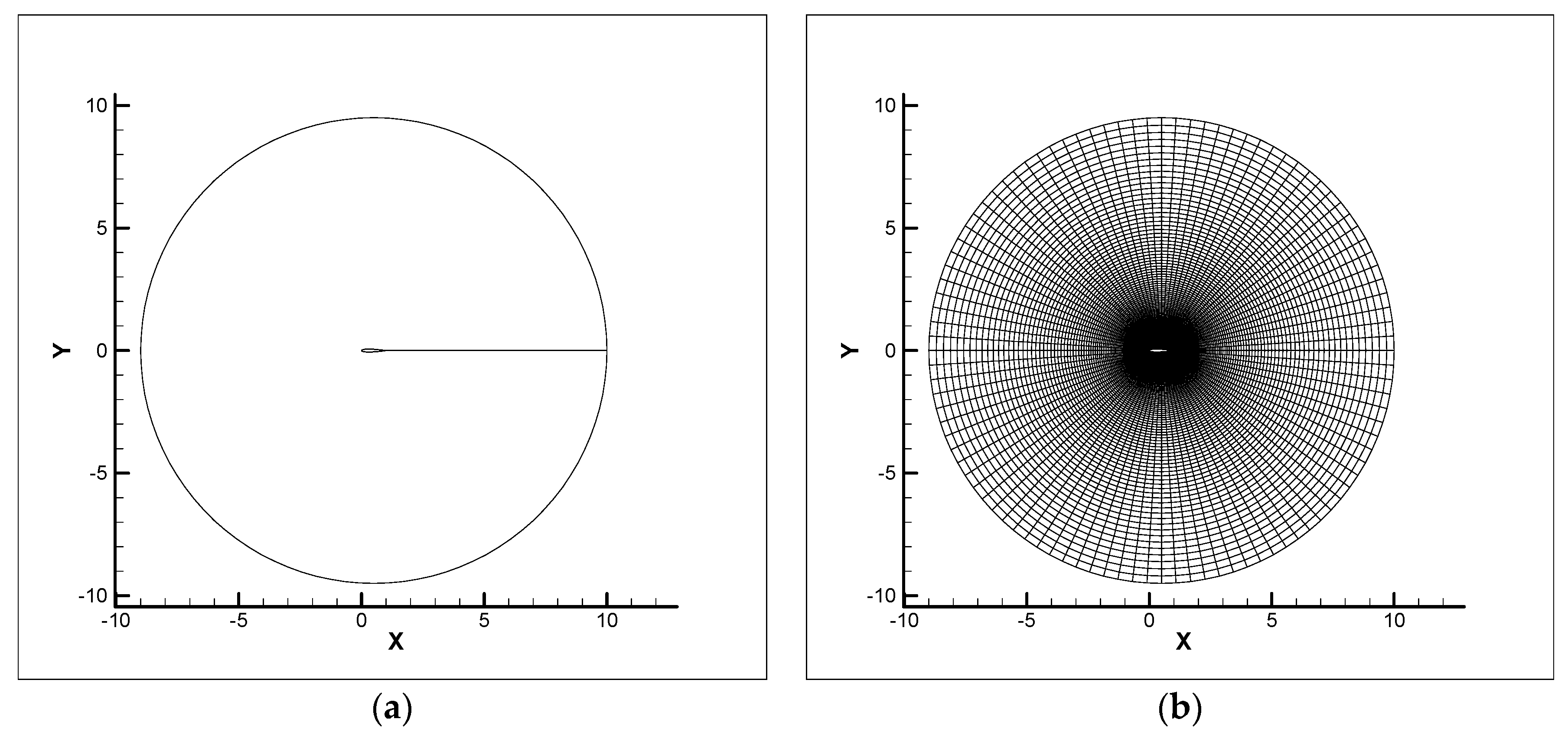
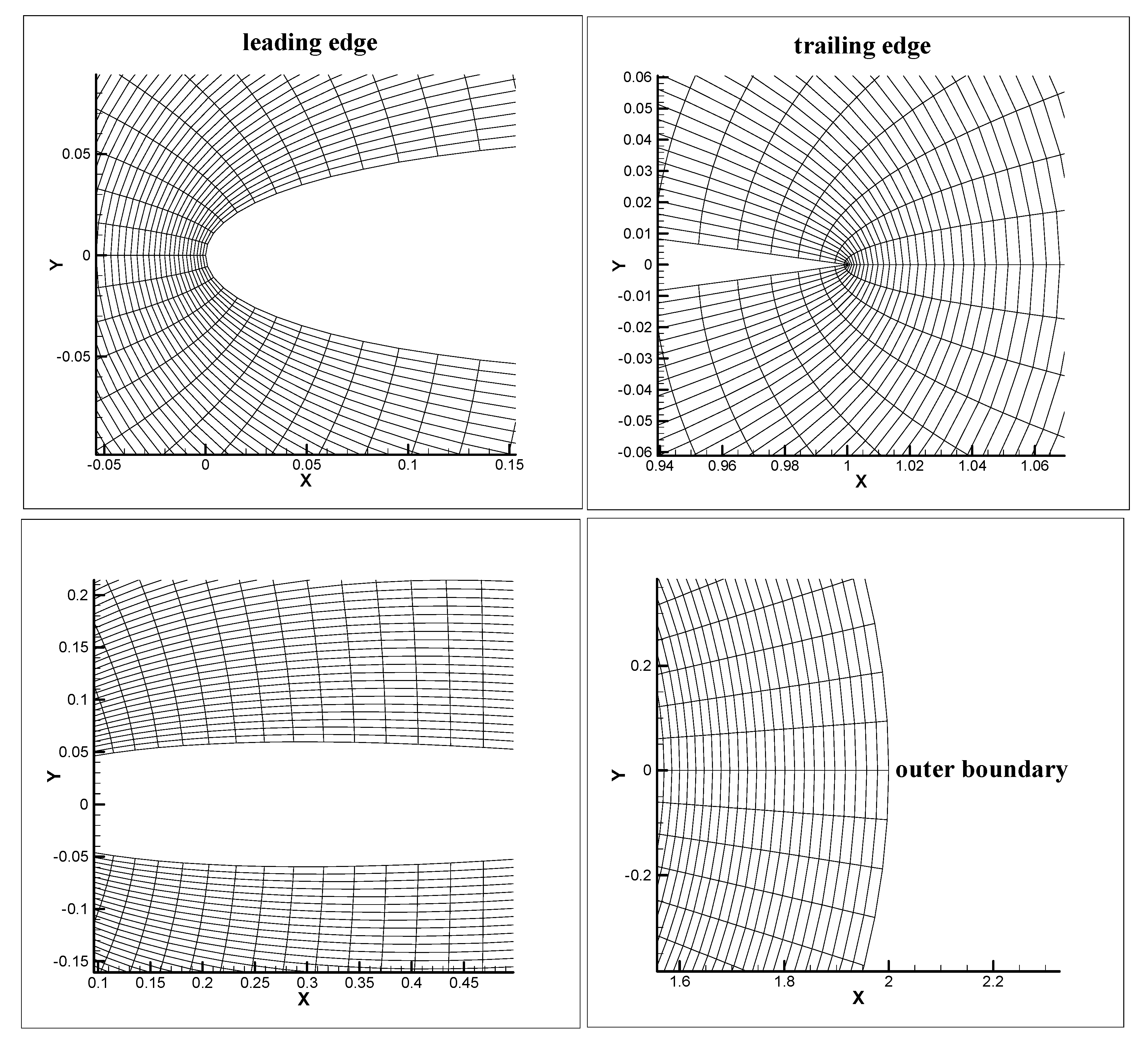
Here, an O-grid is initially generated around the airfoil using elliptic grid generation method [17] and then the stream function equation is solved in the computational domain. The size of mesh is $M\times N$ where $M$ is the number of nodes on the branch cut (a horizontal line connecting the trailing edge to outer boundary) and $N$ is the number of nodes on the airfoil surface (and hence, the outer boundary), as shown in Figure 1. The physical domain before and after meshing using an O-grid of size $110\times 101$ is shown in Figure 2 (using a NACA 0012 airfoil). Moreover, the magnified view of different parts of domain is shown in Figure 3 to highlight the orthogonality of the gridlines at airfoil surface and outer boundary.

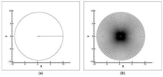
Figure 2. The physical domain before and after meshing. (a) Physical domain before meshing. (b) Physical domain after meshing.

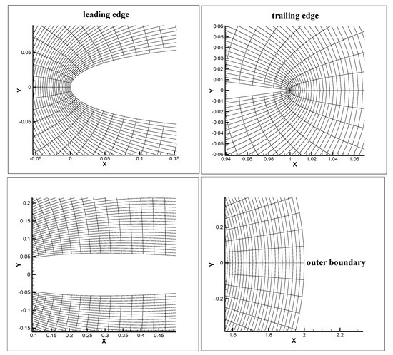
Figure 3. Magnified view of different parts of domain.

2.4. Kutta Condition

In inviscid flows, because the flow cannot penetrate the surface, the velocity vector must be tangential to the surface. In other words, the component of velocity normal to the surface must be zero and only the tangential velocity component must be considered. The unit tangent vector on the airfoil surface can be expressed as

$${\mathsf{\tau }}^{(\xi )}={\mathbf{n}}^{(\xi )}\times \mathbf{k}$$

(35)

$${\mathsf{\tau }}^{(\eta )}={\mathbf{n}}^{(\eta )}\times \mathbf{k}$$

(36)

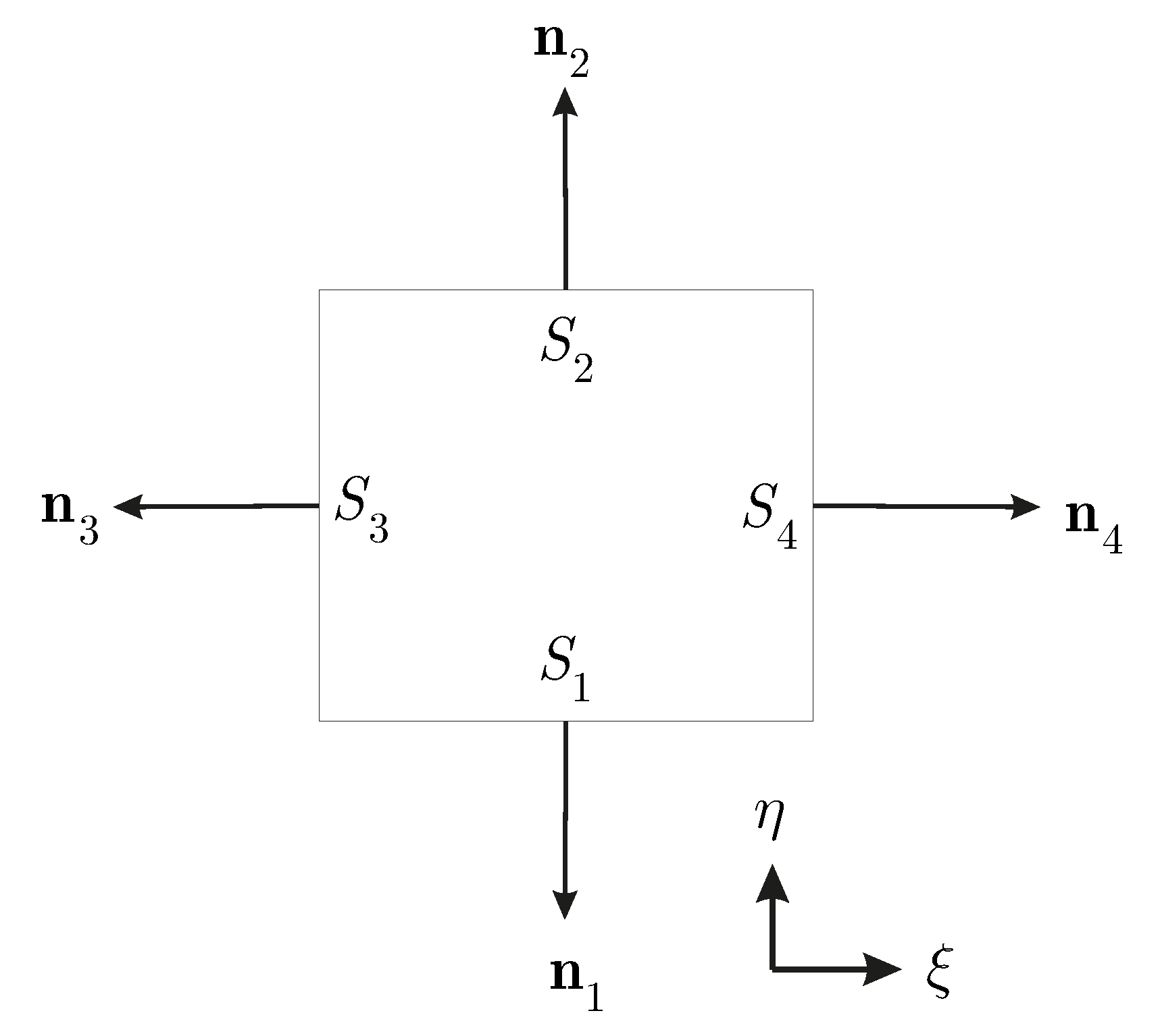
where ${\mathbf{n}}^{(\xi )}$ and ${\mathbf{n}}^{(\eta )}$ are the outward-pointing unit normal vector to a airfoil surface in $\xi$ and $\eta$ directions, respectively, and $\mathbf{k}$ is the unit vector in $z$ direction.

At the airfoil surface, corresponding to surface $S_3$ in Figure 4, we have

$${\mathbf{n}}^{(\xi )}=-\frac{\nabla \xi }{\left|\nabla \xi \right|}=-\frac{{\xi }_x\mathbf{i}+{\xi }_y\mathbf{j}}{\sqrt{{\xi }_x^2+{\xi }_y^2}}$$

(37)

Figure 4. The outward—pointing unit normal vectors to $\xi$ = constant and $\eta$ = constant lines.

From the transformation relationships (Equation (19)), we have

$${\mathbf{n}}^{(\xi )}=-\frac{\frac{1}{J}{y}_{\eta }\mathbf{i}+(-\frac{1}{J}{x}_{\eta }\mathbf{j})}{\sqrt{{(\frac{y_{\eta }}{J})}^2+{(-\frac{x_{\eta }}{J})}^2}}=\frac{-y_{\eta }\mathbf{i}+x_{\eta }\mathbf{j}}{\sqrt{\alpha }}$$

(38)

where $\alpha =x_{\eta }{}^2+y_{\eta }{}^2$. Using Equation (35), we get

$${\mathsf{\tau }}_{S_3}^{{}^{(\xi )}}={\mathbf{n}}_{S_3}^{{}^{(\xi )}}\times \mathbf{k}=\frac{1}{\sqrt{\alpha }}(-y_{\eta }\mathbf{i}+x_{\eta }\mathbf{j})\times \mathbf{k}=\frac{1}{\sqrt{\alpha }}(-y_{\eta }(-\mathbf{j})+x_{\eta }\mathbf{i})=\frac{1}{\sqrt{\alpha }}(x_{\eta }\mathbf{i}+y_{\eta }\mathbf{j})$$

(39)

The velocity component tangential to the airfoil surface ($S_3$) is

$$V_t=\mathbf{V}.{\mathsf{\tau }}_{S_3}^{(\xi )}=(u\mathbf{i}+v\mathbf{j}).\frac{1}{\sqrt{\alpha }}(x_{\eta }\mathbf{i}+y_{\eta }\mathbf{j})$$

(40)

For compressible flows, the velocity components of $u$ and $v$ can be expressed in terms of stream function $\psi$ as

$$u=\frac{{\rho }_0}{\rho }{\psi }_y=\frac{{\rho }_0}{\rho }\frac{1}{J}(-x_{\eta }{\psi }_{\xi }+x_{\xi }{\psi }_{\eta })$$

(41)

and

$$v=-\frac{{\rho }_0}{\rho }{\psi }_x=-\frac{{\rho }_0}{\rho }\frac{1}{J}(y_{\eta }{\psi }_{\xi }-y_{\xi }{\psi }_{\eta })$$

(42)

where ${\rho }_0$ is a constant. On the airfoil surface, ${\psi }_s={\psi }_{\eta }=0$ where $s$ is the distance measured along the airfoil surface because the airfoil contour is a streamline of the flow. Thus Equations (41) and (42) become

$$u=\frac{{\rho }_0}{\rho }\frac{1}{J}(-x_{\eta }{\psi }_{\xi })$$

(43)

and

$$v=-\frac{{\rho }_0}{\rho }\frac{1}{J}(y_{\eta }{\psi }_{\xi })$$

(44)

By substituting Equations (43) and (44) into Equation (40), we get

$$\begin{gathered} V_t=(-\frac{{\rho }_0}{\rho }\frac{1}{J}{x}_{\eta }{\psi }_{\xi }\mathbf{i}-\frac{{\rho }_0}{\rho }\frac{1}{J}{y}_{\eta }{\psi }_{\xi }\mathbf{j}).\frac{1}{\sqrt{\alpha }}(x_{\eta }\mathbf{i}+y_{\eta }\mathbf{j})=-\frac{{\rho }_0}{\rho }\frac{1}{J}\frac{1}{\sqrt{\alpha }}{x}_{\eta }^2{\psi }_{\xi }-\frac{{\rho }_0}{\rho }\frac{1}{J}\frac{1}{\sqrt{\alpha }}{y}_{\eta }^2{\psi }_{\xi }= \\ -\frac{{\rho }_0}{\rho }\frac{1}{J}\frac{1}{\sqrt{\alpha }}(x_{\eta }^2+y_{\eta }^2){\psi }_{\xi }=-\frac{{\rho }_0}{\rho }\frac{1}{J}\frac{1}{\sqrt{\alpha }}(\alpha ){\psi }_{\xi }=-\frac{{\rho }_0}{\rho }\frac{\sqrt{\alpha }}{J}{\psi }_{\xi } \end{gathered}$$

(45)

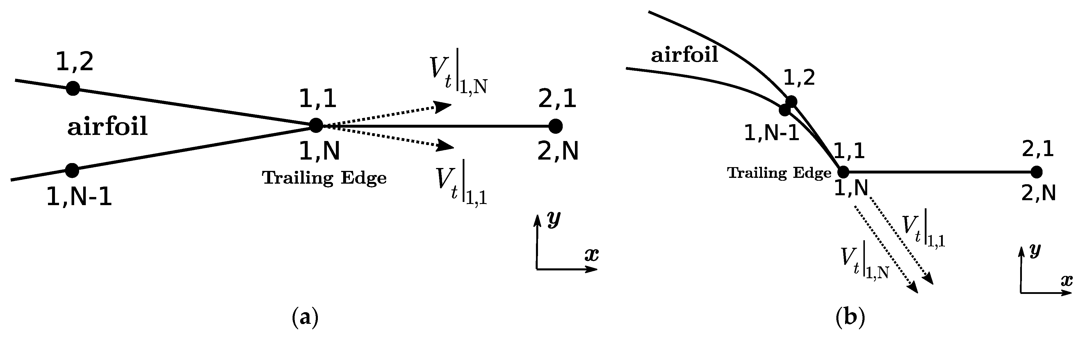
Based on the Kutta condition, the velocity at the trailing edge of the airfoil must be the same when approached from the upstream direction along the upper and lower airfoil surfaces [20] (see Figure 5). Thus,

$${V_t|}_{{}_{1,1}}={V_t|}_{{}_{1,\mathrm{N}}}=C\{\begin{array}{l}C=0\hspace{1em}\hspace{1em} \mathrm{for} \mathrm{finite} \mathrm{angle} \mathrm{trailing} \mathrm{edge}\\ C\ne 0\hspace{1em}\hspace{1em} \mathrm{for} \mathrm{cusped} \mathrm{trailing} \mathrm{edge}\end{array}$$

(46)

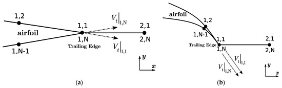
Figure 5. Grid notation and tangential velocity components at trailing edge. (a) Finite angle trailing edge. (b) Cusped trailing edge.

For the finite angle trailing edge, we have

$${V_t|}_{{}_{1,1}}=0$$

$${-\frac{{\rho }_0}{\rho }\frac{\sqrt{\alpha }}{J}{\psi }_{\xi }|}_{{}_{1,1}}=0$$

hence

$$\begin{gathered} {{\psi }_{\xi }|}_{1,1}=0 \\ {\psi }_{2,1}-{\psi }_{1,1}=0 \end{gathered}$$

$${\psi }_{2,1}={\psi }_{1,1}$$

(47)

(The above expression is based on forward finite-difference coefficient with first-order accuracy. The forward finite-difference coefficient with second-order accuracy can be used if more accurate Kutta condition implementation is needed.)

Therefore, the wall boundary condition for the finite angle trailing edge becomes

$${\psi }_{1,j}={\psi }_{2,1}(j=1,\dots ,N)$$

(48)

because the stream function on the airfoil surface is constant.

For the cusped trailing edge, we have

$$\begin{gathered} {V_t|}_{1,1}={V_t|}_{1,\mathrm{N}} \\ {-\frac{{\rho }_0}{\rho }\frac{\sqrt{\alpha }}{J}{\psi }_{\xi }|}_{{}_{1,1}}={-\frac{{\rho }_0}{\rho }\frac{\sqrt{\alpha }}{J}{\psi }_{\xi }|}_{1,\mathrm{N}} \end{gathered}$$

(49)

The points $(1,1)$ and $(1,\mathrm{N})$ as well as the points $(2,1)$ and $(2,\mathrm{N})$ are the same points (see Figure 5). Therefore, ${\psi }_{1,1}={\psi }_{1,\mathrm{N}}$ and ${\psi }_{2,1}={\psi }_{2,\mathrm{N}}$

$${{\psi }_{\xi }|}_{1,1}={\psi }_{2,1}-{\psi }_{1,1}={\psi }_{2,\mathrm{N}}-{\psi }_{1,\mathrm{N}}={{\psi }_{\xi }|}_{1,\mathrm{N}}$$

On the other hand, we know that

$${-\frac{{\rho }_0}{\rho }\frac{\sqrt{\alpha }}{J}|}_{{}_{1,1}}\ne {-\frac{{\rho }_0}{\rho }\frac{\sqrt{\alpha }}{J}|}_{1,\mathrm{N}}$$

(50)

Thus, the only possibility to satisfy Equation (49) is that

$${{\psi }_{\xi }|}_{1,1}={{\psi }_{\xi }|}_{1,\mathrm{N}}=0$$

which this relation again results in the same expression as for the finite angle trailing edge case. So, the general expression to implement the Kutta condition based on the stream function for the 2D compressible flow is

$${\psi }_{1,1}={\psi }_{2,1}$$

(51)

which is the same as one for the incompressible flow [21]

2.5. Computation Procedure

According to the mapping scheme adopted in Figure 1, there are four sections where the nodal value of the flow variables $f_{i,j}$ ($f\equiv \psi ,\rho ,p,u,v,V,c,M,\dots$) should be calculated.

• Inside the domain to calculate the variables $f_{i,j}$ ($i=2,\dots ,M-1$, $j=2,\dots ,N-1$).
• On the airfoil surface to calculate the variables $f_{1,j}$ ($j=1,\dots ,N$).
• At the outer boundary (far-field) to calculate the variables $f_{M,j}$ ($j=1,\dots ,N$).
• On the branch cut to calculate the variables $f_{i,1}$ ($i=2,\dots ,M-1$). We know that $f_{i,N}=f_{i,1}$.

The known free-stream variables are $M_{\infty }$, $p_{\infty }$, ${\rho }_{\infty }$, $T_{\infty }$, and the angle of attack $\alpha$. Thus, we can write

$$M_{M,j}=M_{\infty }(j=1,\dots ,N)$$

(52)

$$T_{M,j}=T_{\infty }(j=1,\dots ,N)$$

(53)

$${\rho }_{M,j}={\rho }_{\infty }(j=1,\dots ,N)$$

(54)

$$p_{M,j}=p_{\infty }(j=1,\dots ,N)$$

(55)

$$c_{M,j}=c_{\infty }=\sqrt{{\gamma }_{\mathrm{air}}{R}_{\mathrm{air}}{T}_{\infty }}=\sqrt{(1.4)(287)T_{M,j}}\hspace{1em}(j=1,\dots ,N)$$

(56)

$$V_{M,j}=V_{\infty }=M_{\infty }{c}_{\infty }=M_{M,j}{c}_{M,j}\hspace{1em}(j=1,\dots ,N)$$

(57)

from the local isentropic stagnation properties of an ideal gas, we have

$$\frac{{\rho }_{0_{M,j}}}{{\rho }_{M,j}}={(1+\frac{{\gamma }_{\mathrm{air}}-1}{2}{M}_{M,j}^2)}^{\frac{1}{{\gamma }_{\mathrm{air}}-1}}\hspace{1em}(j=1,\dots ,N)$$

(58)

so the local total density ${\rho }_{0_{M,j}}$ can be computed as

$${\rho }_{0_{M,j}}={\rho }_{M,j}{(1+\frac{{\gamma }_{\mathrm{air}}-1}{2}{M}_{M,j}^2)}^{\frac{1}{{\gamma }_{\mathrm{air}}-1}}\hspace{1em}(j=1,\dots ,N)$$

(59)

In a similar fashion, we can write

$$p_{0_{M,j}}=p_{M,j}{(1+\frac{{\gamma }_{\mathrm{air}}-1}{2}{M}_{M,j}^2)}^{\frac{{\gamma }_{\mathrm{air}}}{{\gamma }_{\mathrm{air}}-1}}\hspace{1em}(j=1,\dots ,N)$$

(60)

$$T_{0_{M,j}}=T_{M,j}(1+\frac{{\gamma }_{\mathrm{air}}-1}{2}{M}_{M,j}^2)\hspace{1em}(j=1,\dots ,N)$$

(61)

$$c_{0_{M,j}}=\sqrt{{\gamma }_{\mathrm{air}}{R}_{\mathrm{air}}{T}_{0_{M,j}}}=\sqrt{(1.4)(287)T_{0_{M,j}}}\hspace{1em}(j=1,\dots ,N)$$

(62)

We know that if the general flow field is isentropic throughout, then the local total density ${\rho }_0$, the local total pressure $p_0$, and the local total temperature $T_0$ are constant values throughout the flow. Thus

$$c_{0_{i,j}}=c_{0_{M,j}}\hspace{1em}(i=1,\dots ,M,j=1,\dots ,N)$$

(63)

$${\rho }_{0_{i,j}}={\rho }_{0_{M,j}}\hspace{1em}(i=1,\dots ,M,j=1,\dots ,N)$$

(64)

$$p_{0_{i,j}}=p_{0_{M,j}}\hspace{1em}(i=1,\dots ,M,j=1,\dots ,N)$$

(65)

$$T_{0_{i,j}}=T_{0_{M,j}}\hspace{1em}(i=1,\dots ,M,j=1,\dots ,N)$$

(66)

Also, on the outer boundary (far-field) we have

$$u_{M,j}=V_{x_{\infty }}=V_{\infty }\cos \alpha \hspace{1em}(j=1,\dots ,N)$$

(67)

$$v_{M,j}=V_{y_{\infty }}=V_{\infty }\sin \alpha \hspace{1em}(j=1,\dots ,N)$$

(68)

If the number of nodes on the outer boundary (the side $BG$ in Figure 1) is $N$, then, as shown in Figure 6, the node number of two points at top (point $E$) and bottom (point $F$) of the circular outer boundary would be $(M,\frac{N+3}{4})$ and $(M,\frac{3N+1}{4})$, respectively.

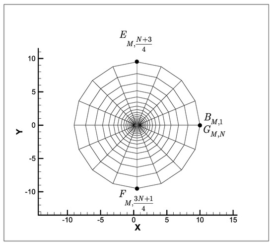
Figure 6. Representation of node number of top and bottom points on the outer boundary (far-field).

Then we can express the magnitude of the stream function on the outer boundary ${\psi }_{M,j}$ in terms of far-field velocity $V_{M,j}$ as (by considering the equal magnitudes but opposite in sign for stream functions at top and bottom points of $E$ and $F$, that is, ${\psi }_F=-c$ and ${\psi }_E=c$, $c$ is a constant)

$$\begin{gathered} u_{M,\frac{3N+1}{4}}=\frac{{\rho }_{0_{M,\frac{3N+1}{4}}}}{{\rho }_{M,\frac{3N+1}{4}}}{\frac{\partial \psi }{\partial y}|}_{M,\frac{3N+1}{4}}=\frac{{\rho }_{0_{M,\frac{3N+1}{4}}}}{{\rho }_{M,\frac{3N+1}{4}}}(\frac{{\psi }_{M,\frac{N+3}{4}}-{\psi }_{M,\frac{3N+1}{4}}}{y_{M,\frac{N+3}{4}}-y_{M,\frac{3N+1}{4}}})= \\ \frac{{\rho }_{0_{M,\frac{3N+1}{4}}}}{{\rho }_{M,\frac{3N+1}{4}}}(\frac{-{\psi }_{M,\frac{3N+1}{4}}-{\psi }_{M,\frac{3N+1}{4}}}{y_{M,\frac{N+3}{4}}-y_{M,\frac{3N+1}{4}}})=-\frac{{\rho }_{0_{M,\frac{3N+1}{4}}}}{{\rho }_{M,\frac{3N+1}{4}}}(\frac{2{\psi }_{M,\frac{3N+1}{4}}}{y_{M,\frac{N+3}{4}}-y_{M,\frac{3N+1}{4}}}) \end{gathered}$$

(69)

Therefore,

$${\psi }_{M,\frac{3N+1}{4}}=-\frac{{\rho }_{M,\frac{3N+1}{4}}}{{\rho }_{0_{M,\frac{3N+1}{4}}}}{u}_{M,\frac{3N+1}{4}}\frac{y_{M,\frac{N+3}{4}}-y_{M,\frac{3N+1}{4}}}{2}$$

(70)

Now the magnitude of the stream function on the outer boundary can be calculated as a (based on the relation $\psi =-\frac{\rho }{{\rho }_0}{V}_{y}x+\frac{\rho }{{\rho }_0}{V}_{x}y$)

$${\psi }_{M,j}={\psi }_{M,\frac{3N+1}{4}}+\frac{{\rho }_{M,j}}{{\rho }_{0_{M,j}}}{u}_{M,j}(y_{M,j}-y_{M,\frac{3N+1}{4}})-\frac{{\rho }_{M,j}}{{\rho }_{0_{M,j}}}{v}_{M,j}(x_{M,j}-x_{M,\frac{3N+1}{4}})$$

(71)

In Equation (69), we should note that the two points $E$ and $F$ have the same $x$-coordinates and hence $\psi =-\frac{\rho }{{\rho }_0}{V}_{y}x+\frac{\rho }{{\rho }_0}{V}_{x}y=0+\frac{\rho }{{\rho }_0}{V}_{x}y=\frac{\rho }{{\rho }_0}{V}_{x}y$.

The iterative process to obtain the value of ${\psi }_{i,j}$ and ${\rho }_{i,j}$ may be initiated by assuming $\frac{{\rho }_{0_{i,j}}}{{\rho }_{i,j}}=1$ or ${\rho }_{i,j}={\rho }_{0_{i,j}}$. This initial assumption implies that the magnitude of the speed of sound is infinite ($c=\infty \Rightarrow \frac{1}{c^2}=0$) and Equation (5) reduces to Laplace’s equation

$${\psi }_{xx}+{\psi }_{yy}=0$$

(72)

The first iteration is concerned with the solution of Laplace’s equation which is described thoroughly in [21] and we do not elaborate further on it. After solving the Laplace’s equation to find the value of the stream function at each node, ${\psi }_{i,j}$, in the flow field, the values of the velocity components of $u_{i,j}$ and $v_{i,j}$ can be computed from Equations (2) and (3). Then, the value of the speed of sound at each node, $c_{i,j}$,can be calculated from Equation (4). Finally, the value of the density at each node, ${\rho }_{i,j}$, can be determined from Equation (7). If the flow is compressible, ${\rho }_{i,j}\ne {\rho }_{0_{i,j}}$ and from the second iteration onwards, instead of Laplace’s equation, the stream function given in Equation (6) must be solved by having the density ${\rho }_{i,j}$ and the stream function ${\psi }_{i,j}$ from the last iteration (i.e., iteration 1) to get new values of the stream function ${\psi }_{i,j}$. The iterative process (solving Equations (6) and (7) simultaneously) repeated until successive iterations produce a sufficiently small change in density ${\rho }_{i,j}$ and the stream function ${\psi }_{i,j}$. Equation (6) is solved by initially discretizing the partial differential terms in Equations (21)–(26) using relations given in Equations (27)–(31) and then substituting the terms into Equation (6), and finally, solving the obtained algebraic equation using an algebraic solver (such as Maple) to get an explicit algebraic expression in terms of ${\psi }_{i,j}$. As stated before, the Kutta condition is implemented as

$${\psi }_{1,1}={\psi }_{2,1}$$

(73)

$${\psi }_{1,N}={\psi }_{1,1}\hspace{1em}\hspace{1em}(\mathrm{the}\mathrm{same}\mathrm{node})$$

(74)

and the wall boundary condition is implemented as

$${\psi }_{1,j}={\psi }_{1,j-1}\hspace{1em}\hspace{1em}(j=2,\dots ,N-1)$$

(75)

and since the branch cut ($AB$ or $HG$ in Figure 1) is inside the flow field, the same procedure employed to obtain an algebraic expression for ${\psi }_{i,j}$ can also be used to obtain an expression for the stream function on the branch cut, ${\psi }_{i,1}$. However, some changes are needed in the terms discretized by the finite-difference method (Equations (27)–(31)) as follows (see Figure 7)

$${(f_{\xi })}_{i,1}=\frac{1}{2}(f_{i+1,1}-f_{i-1,1})$$

(76)

$${(f_{\eta })}_{i,1}=\frac{1}{2}(f_{i,2}-f_{i,N-1})$$

(77)

$${(f_{\xi \xi })}_{i,1}=(f_{i+1,1}-2f_{i,1}+f_{i-1,1})$$

(78)

$${(f_{\eta \eta })}_{i,1}=(f_{i,2}-2f_{i,1}+f_{i,N-1})$$

(79)

$${(f_{\xi \eta })}_{i,1}=\frac{1}{4}(f_{i+1,2}-f_{i-1,2}-f_{i+1,N-1}+f_{i-1,N-1})$$

(80)

where $f\equiv x,y,\psi$.

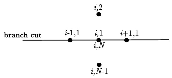
Figure 7. Node notation on the branch cut.

and on the branch cut

$${\psi }_{i,N}={\psi }_{i,1}\hspace{1em}\hspace{1em}(i=2,\dots ,M-1)$$

(81)

In order to solve the elliptic grid generation equations (for $x$ and $y$) and the stream function equation, the iterative method Successive Over Relaxation (SOR) is used due to its high convergence rate

$$f_{i,j}^{(k)}=\omega f_{i,j}^{(k-1)}+(1-\omega )f_{i,j}^{(k-2)}$$

(82)

where $f\equiv x,y,\psi$. In these relation for SOR, $k$ is iteration number, and $\omega$ is relaxation factor which has a value of $1<\omega <2$. A value of $\omega =1.8$ is chosen in this study and the code FOILcom.

We should define the stopping criteria for convergence of solution of the stream function equation (Equation (6) and density equation (Equation (7)). These two equations constitute the system of equations to be solved simultaneously. The stopping criteria are defined as follows

$${\lambda }_{\psi }={\displaystyle \sum _{i=2}^{M-1}{\displaystyle \sum _{j=2}^{N-1}({\psi }_{i,j}^{(k+1)}-{\psi }_{i,j}^{(k)}}{)}^2}$$

(83)

$${\lambda }_{\rho }={\displaystyle \sum _{i=2}^{M-1}{\displaystyle \sum _{j=2}^{N-1}({\rho }_{i,j}^{(k+1)}-{\rho }_{i,j}^{(k)}}{)}^2}$$

(84)

where $k$ is iteration number. A value of ${\lambda }_{\psi }={\lambda }_{\rho }={10}^{-4}$ can be considered to get sufficiently accurate results. The other parameters of interest can also be computed after obtaining the density ${\rho }_{i,j}$ and the stream function ${\psi }_{i,j}$. The components of the velocity at each node, $u_{i,j}$ and $v_{i,j}$, can be computed from

$$u_{i,j}=\frac{{\rho }_{0_{i,j}}}{{\rho }_{i,j}}{{\psi }_y|}_{i,j}=\frac{{\rho }_{0_{i,j}}}{{\rho }_{i,j}}{\frac{1}{J}(-x_{\eta }{\psi }_{\xi }+x_{\xi }{\psi }_{\eta })|}_{i,j}$$

(85)

$$v_{i,j}=-\frac{{\rho }_{0_{i,j}}}{{\rho }_{i,j}}{{\psi }_x|}_{i,j}=-\frac{{\rho }_{0_{i,j}}}{{\rho }_{i,j}}{\frac{1}{J}(y_{\eta }{\psi }_{\xi }-y_{\xi }{\psi }_{\eta })|}_{i,j}$$

(86)

Then, the velocity at each node, $V_{i,j}$, is given by

$$V_{i,j}=\sqrt{u_{i,j}^2+v_{i,j}^2}$$

(87)

and the local (nodal) Mach number can be obtained by

$$M_{i,j}=\frac{V_{i,j}}{c_{i,j}}$$

(88)

where the local speed of sound,$c_{i,j}$, is calculated from Equation (4). And finally, the local pressure, $p_{i,j}$, is calculated from

$$\frac{p_{0_{i,j}}}{p_{i,j}}={(1+\frac{{\gamma }_{\mathrm{air}}-1}{2}{M}_{i,j}^2)}^{\frac{{\gamma }_{\mathrm{air}}}{{\gamma }_{\mathrm{air}}-1}}$$

(89)

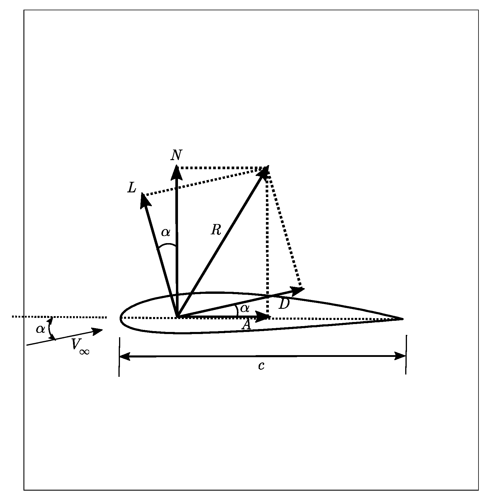
Now the values of drag and lift forces on the airfoil can be computed as follows

$$D=A\cos \alpha +N\sin \alpha$$

(90)

$$L=-A\sin \alpha +N\cos \alpha$$

(91)

where $A$ and $N$ are axial and normal forces, respectively (Figure 8) [4]. We can write the drag and lift forces as

$$D={\displaystyle \sum _{j=1}^{N-1}(p_{1,j}(y_{1,j}-y_{1,j+1})\cos \alpha +p_{1,j}(x_{1,j+1}-x_{1,j})\sin \alpha )}$$

(92)

$$L={\displaystyle \sum _{j=1}^{N-1}(-p_{1,j}(y_{1,j}-y_{1,j+1})\sin \alpha +p_{1,j}(x_{1,j+1}-x_{1,j})\cos \alpha )}$$

(93)

and the drag and the lift coefficients may be expressed as

$$c_d=\frac{D}{\frac{1}{2}{\rho }_{\infty }{V}_{\infty }^2}$$

(94)

$$c_l=\frac{L}{\frac{1}{2}{\rho }_{\infty }{V}_{\infty }^2}$$

(95)

Figure 8. Aerodynamic force $R$ and the components into which it splits [4].

Furthermore, the flowchart of the computational procedure is presented in Figure 9.

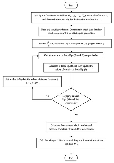
Figure 9. Flowchart of computational procedure.

The theoretical and computational details presented here for compressible flows are implemented in the freely available code FOILcom. Interested readers can refer to the code and use it by changing the airfoil shape, the free stream subcritical Mach number, and the angle of attack. The freely available code FOILincom(DOI: 10.13140/RG.2.2.21727.15524) also takes advantage of the same computational procedure but only for incompressible flow.

3. Results

A few test cases are given to reveal the accuracy and robustness of the numerical scheme. Here, the results from FOILcom are compared with experimental and numerical results (alternative numerical schemes) to show its accuracy and efficiency.

Test case 1: Critical Mach number for the NACA 0012 airfoil at zero angle of attack.

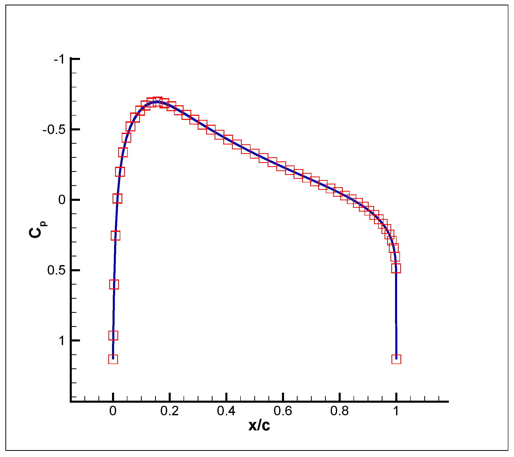
The airfoil surface pressure coefficient distribution using FOILcom is shown in Figure 10. The critical Mach number for the NACA 0012 airfoil at zero angle of attack is obtained as 0.722 using FOILcom with a grid of size $110\times 101$ and $x_{M,1}=10 \mathrm{m}$. The critical Much number in references [4,22] is obtained as 0.725 (the experimental data in [22] is investigated in [4]). A comparison of results is shown in Figure 11 which reveals an excellent agreement.

Figure 10. The pressure coefficient distribution for NACA0012 using FOILcom ($M_{\infty }=M_{\mathrm{critical}}=0.722$, $\alpha =0$).

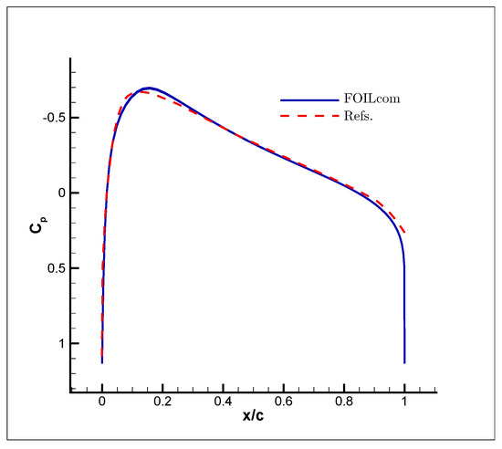
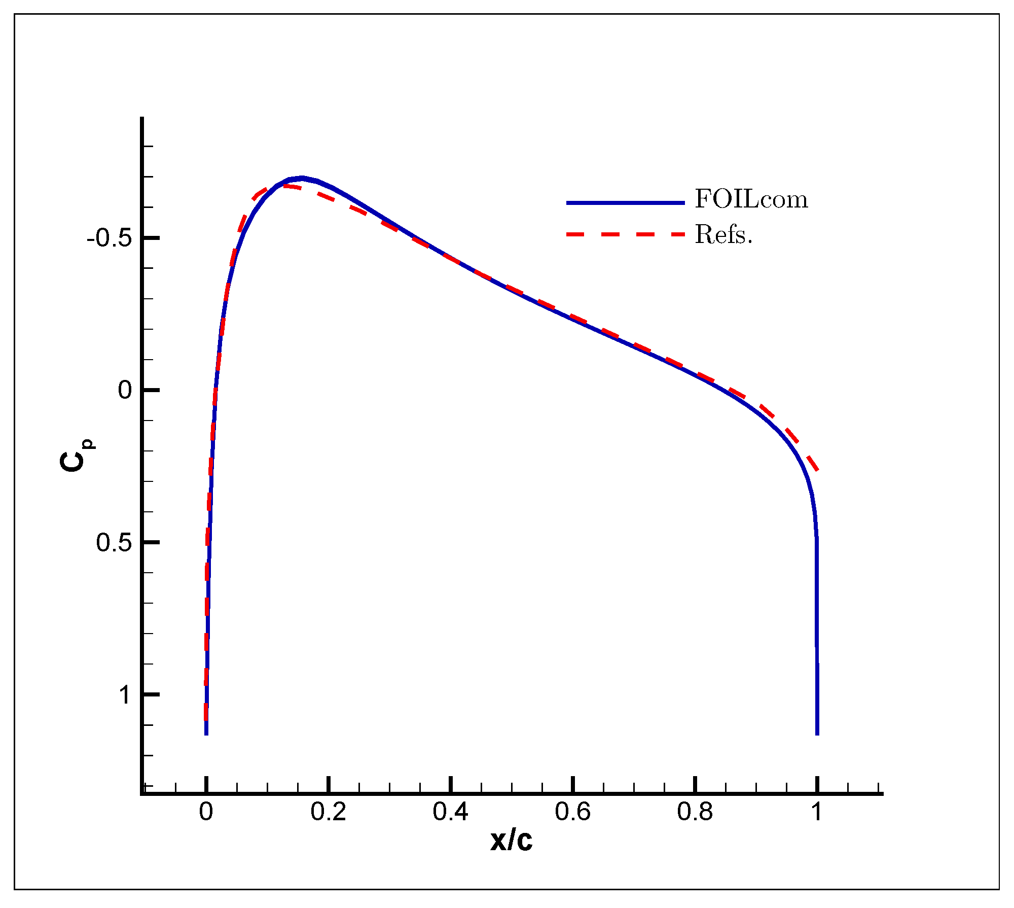
Figure 11. The pressure coefficient distribution. Comparison of FOILcom result and the one from References [4,22].

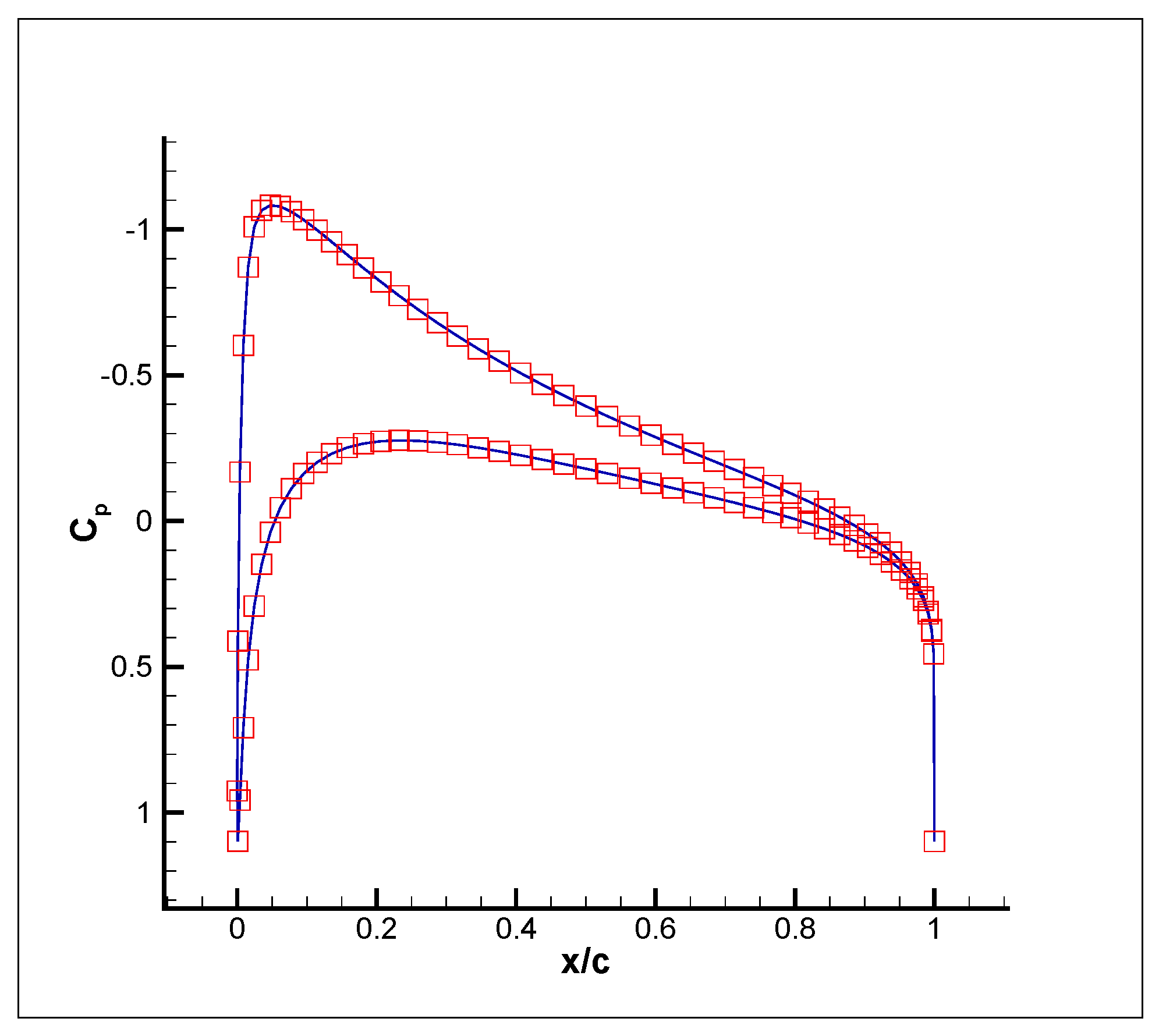
Test case 2: The airfoil surface pressure coefficient distribution for the NACA 0012 using a grid of size $110\times 101$, $M_{\infty }=0.5$, and $\alpha =3^{\circ }$ (Figure 12 and Figure 13). The results from FOILcom (Figure 12) and both finite volume and meshless methods (the results from finite volume and meshless methods in [23] are presented in one plot due to an excellent agreement between the results) are compared and depicted in Figure 13.

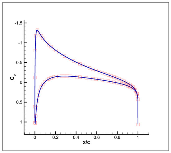
Figure 12. The pressure coefficient distribution for NACA0012 using FOILcom ($M_{\infty }=0.5$, $\alpha =3^{\circ }$).

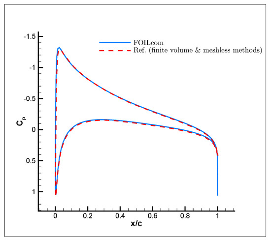
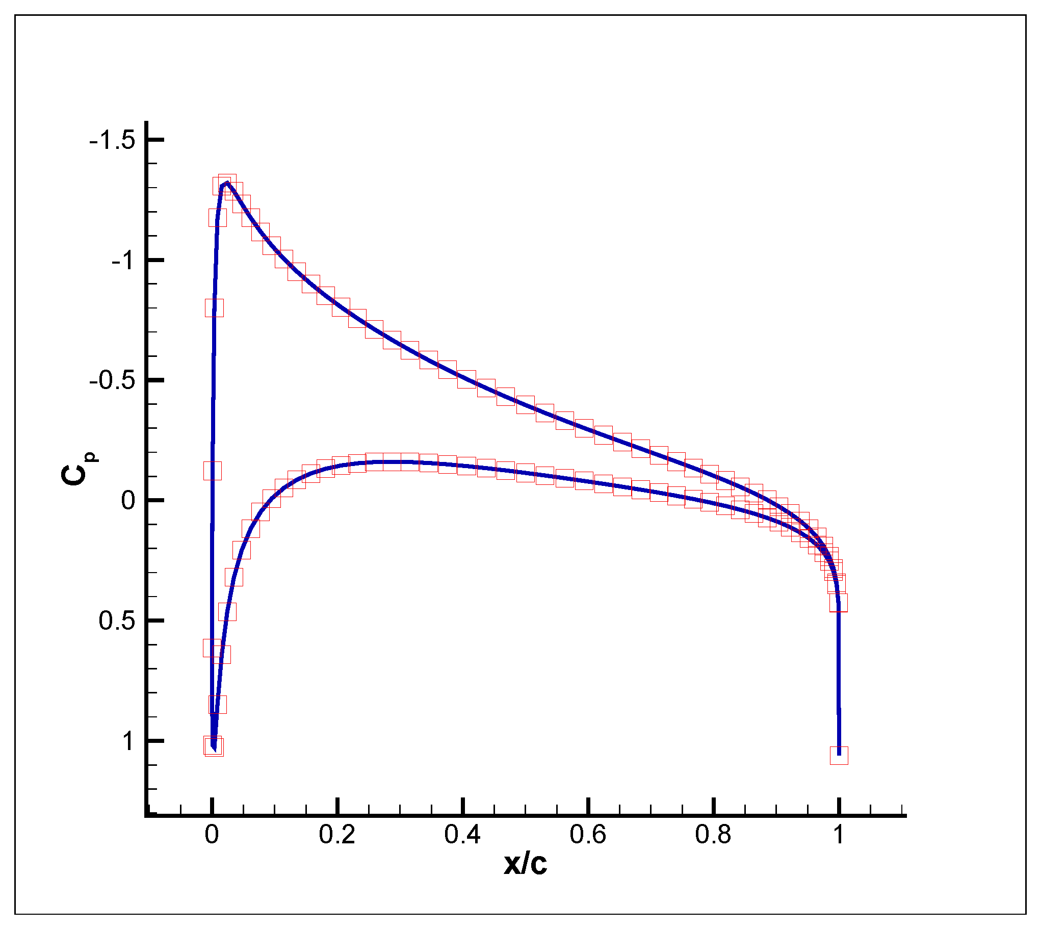
Figure 13. The pressure coefficient distribution. Comparison of FOILcom result and the one from Reference [23].

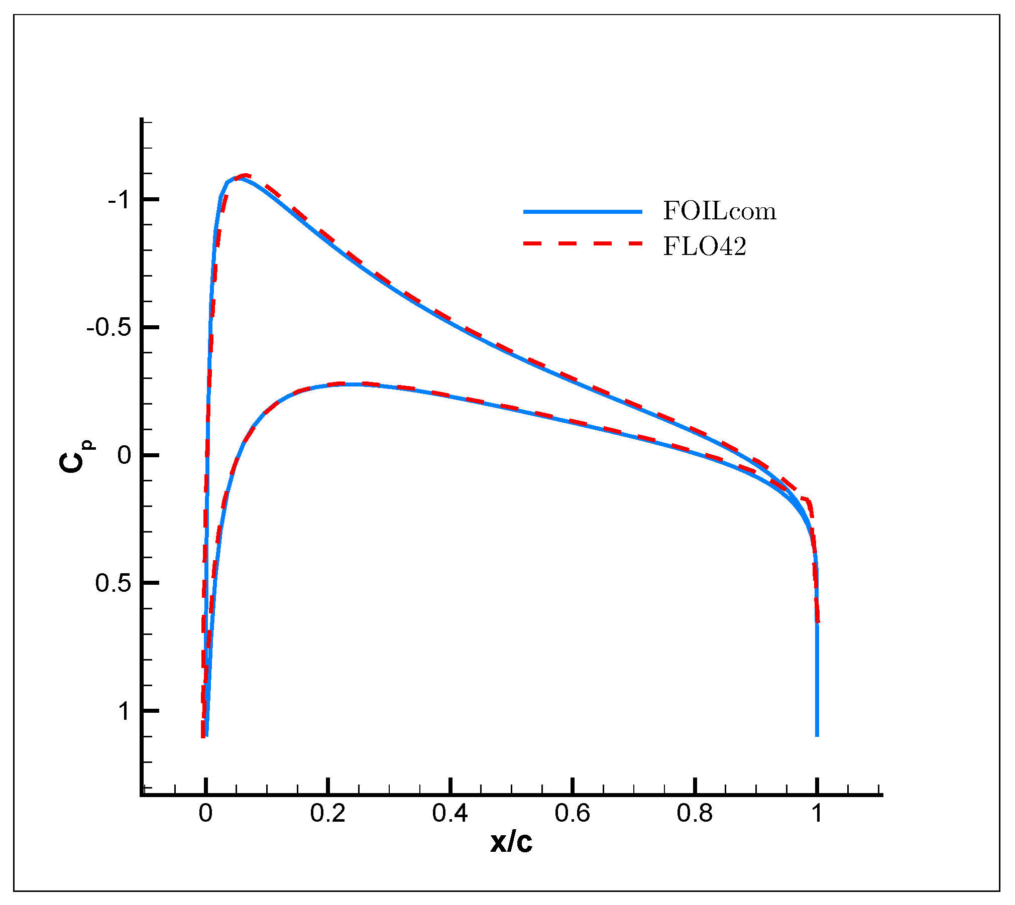
Test case 3: The airfoil surface pressure coefficient distribution for the NACA 0012 using a grid of size $110\times 101$, $M_{\infty }=0.63$, and $\alpha =2^{\circ }$ (Figure 14 and Figure 15). In this test case, the result from FOILcom is compared to the one from the code FLO42. There is excellent agreement between the results.

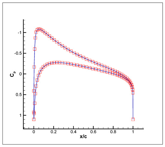
Figure 14. The pressure coefficient distribution for NACA0012 using FOILcom ($M_{\infty }=0.63$, $\alpha =2^{\circ }$).

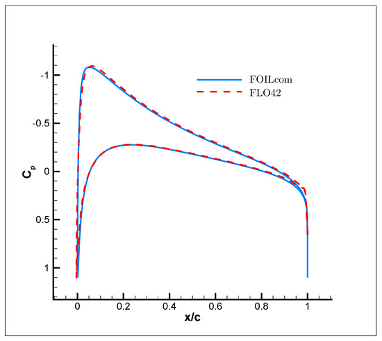
Figure 15. The pressure coefficient distribution. Comparison of FOILcom result and the one from FLO42 [24].

Test case 4: The airfoil surface pressure coefficient distribution for the NACA 2414. $M_{\infty }=0.435$ and $\alpha =2^{\circ }$ (Figure 16 and Figure 17). In this test case, 19,740 nodes (mesh size of $140\times 141$) and 51,792 nodes are used in FOILcom and ANSYS Fluent, respectively. The drag and lift coefficients are calculated as follows:

$$\mathrm{FOILcom}:c_d=-4.362\times {10}^{-}{}^3,c_l=0.573$$

$$\mathrm{ANSYS} \mathrm{Fluent}:c_d=9.985\times {10}^{-}{}^4,c_l=0.574$$

which shows perfect agreement. The results are obtained by a FORTRAN compiler and computations are run on a PC with Intel Core i5 and 6G RAM. A tolerance of ${10}^{-7}$ is used in iterative loops to increase the accuracy of results. The computation time is about 5 min which is high due to the iterative solution of the elliptic grid generation and the stream function equations.

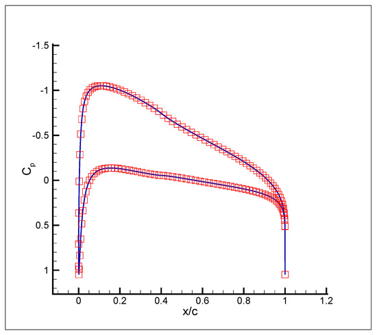
Figure 16. The pressure coefficient distribution for NACA2414 using FOILcom ($M_{\infty }=0.435$, $\alpha =2^{\circ }$).

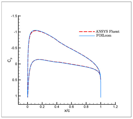
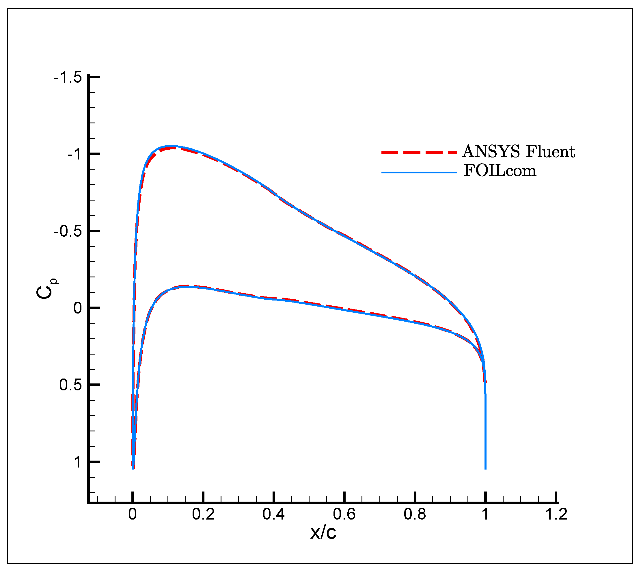
Figure 17. The pressure coefficient distribution. Comparison of FOILcom result and the one from ANSYS Fluent (V19.2).

Test case 5: The airfoil surface pressure coefficient distribution using different grid sizes for NACA 2214 airfoil and $M_{\infty }=0.55$, $\alpha =2^{\circ }$.

Grid sizes are:

(a)

$30\times 41$

(b)

$80\times 61$

(c)

$120\times 161$

(d)

$200\times 201$

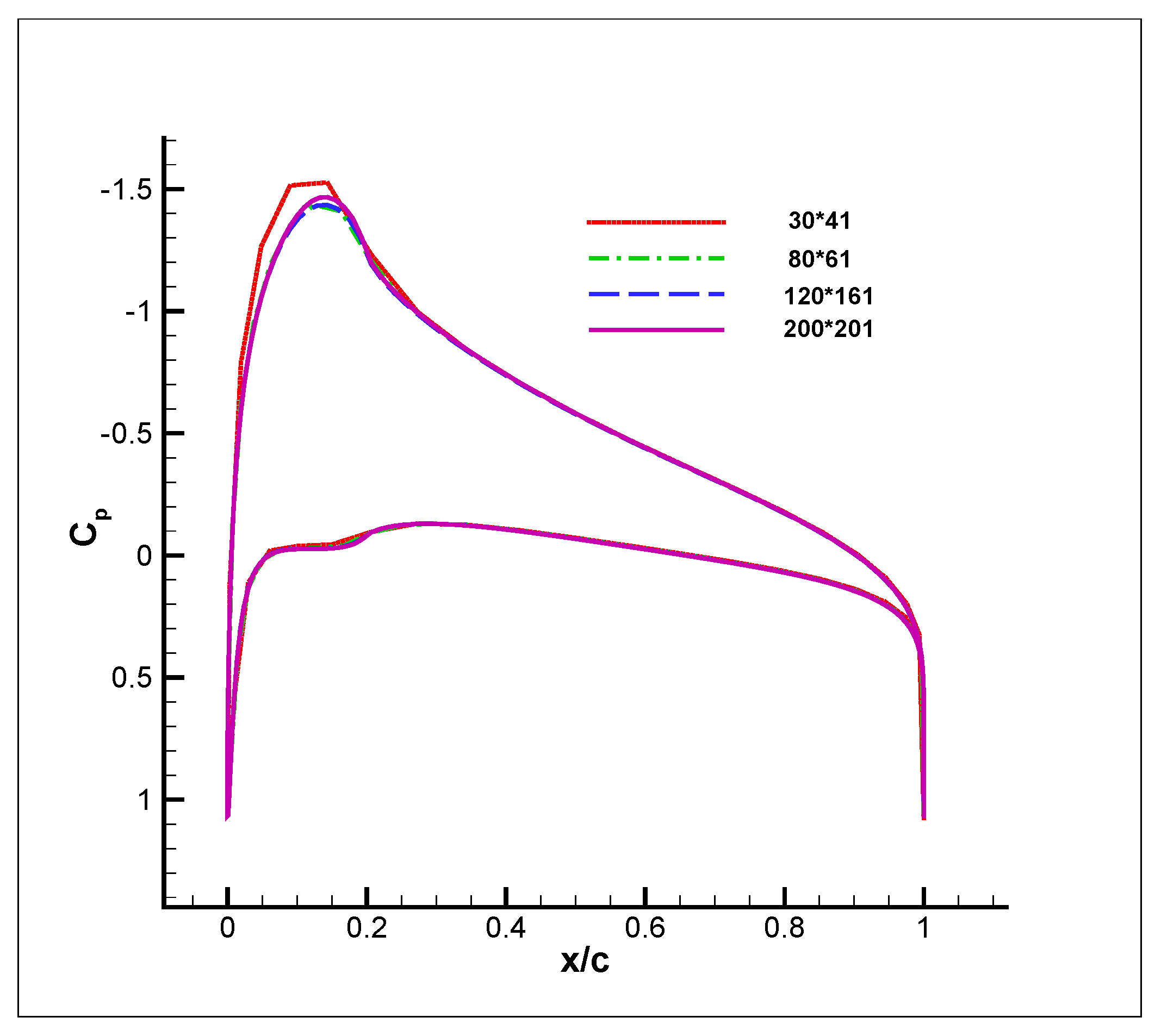
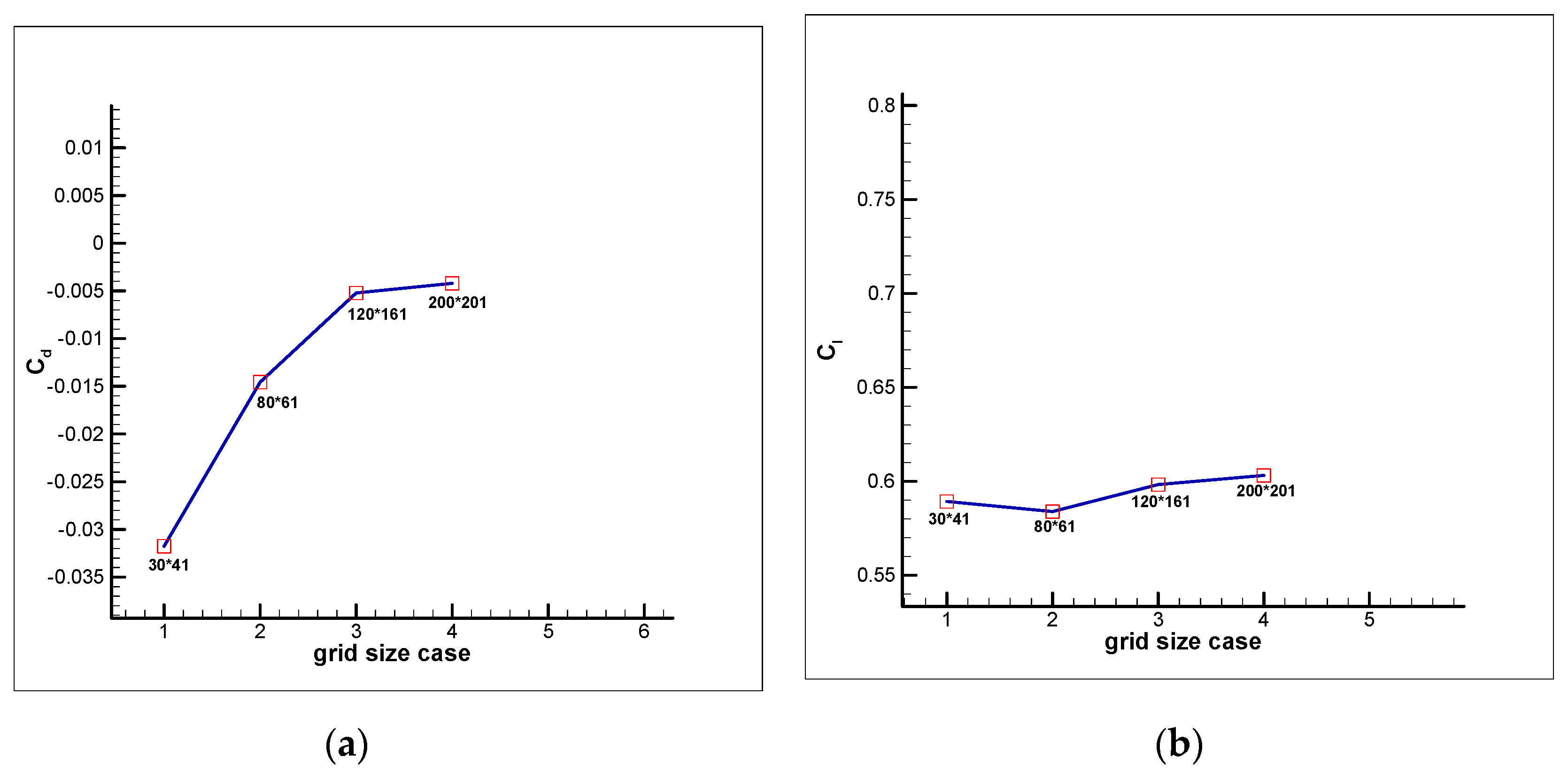
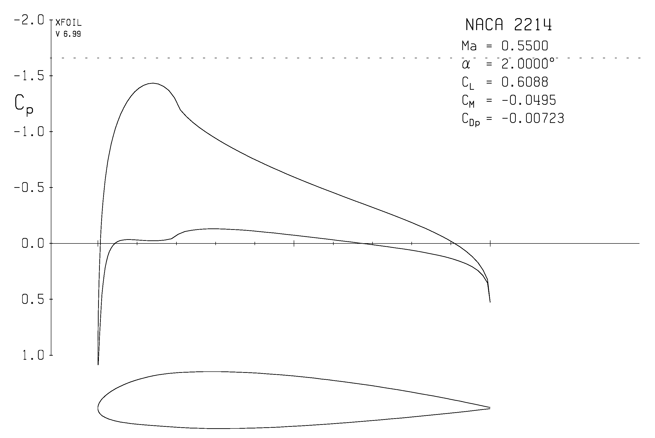
The results are shown in Figure 18. In this test case, four different grid sizes are used to obtain the airfoil surface pressure coefficient distribution. As shown in Figure 18, the distribution can be obtained with reasonable accuracy using even a course grid ($30\times 41$). The effect of grid size on the drag and lift coefficients is depicted in Figure 19. Moreover, the drag and lift coefficients using the four different grid sizes are compared to the ones from XFOIL (Figure 20) and are given in Table 1. As can be seen, the results from FOILcom are in excellent agreement with the result from XFOIL.

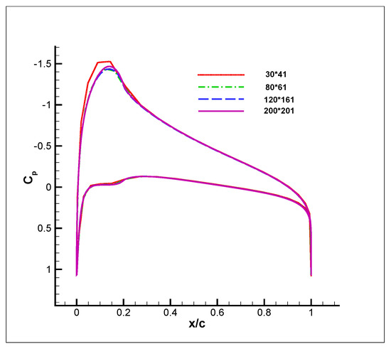
Figure 18. The airfoil surface pressure coefficient distribution using different grid sizes for NACA 2214 airfoil ($M_{\infty }=0.55$, $\alpha =2^{\circ }$). The code FOILcom is used.

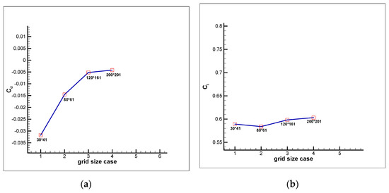
Figure 19. Effect of grid size on drag coefficient (a) and lift coefficient (b).

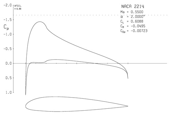
Figure 20. The airfoil surface pressure coefficient distribution for NACA 2214 airfoil ($M_{\infty }=0.55$, $\alpha =2^{\circ }$) using XFOIL.

Table 1. Drag and lift coefficients using different grid sizes. Codes FOILcom and XFOIL are used.

Code and Grid Size	${\mathit{c}}_{\mathit{d}}$	${\mathit{c}}_{\mathit{l}}$
FOILcom: 30 × 41	−3.1764 × 10−2	0.5893
FOILcom: 80 × 61	−1.4563 × 10−2	0.5839
FOILcom: 120 × 161	−5.2130 × 10−3	0.5983
FOILcom: 200 × 201	−4.2097 × 10−3	0.6032
XFOIL	−7.23 × 10−3	0.6088

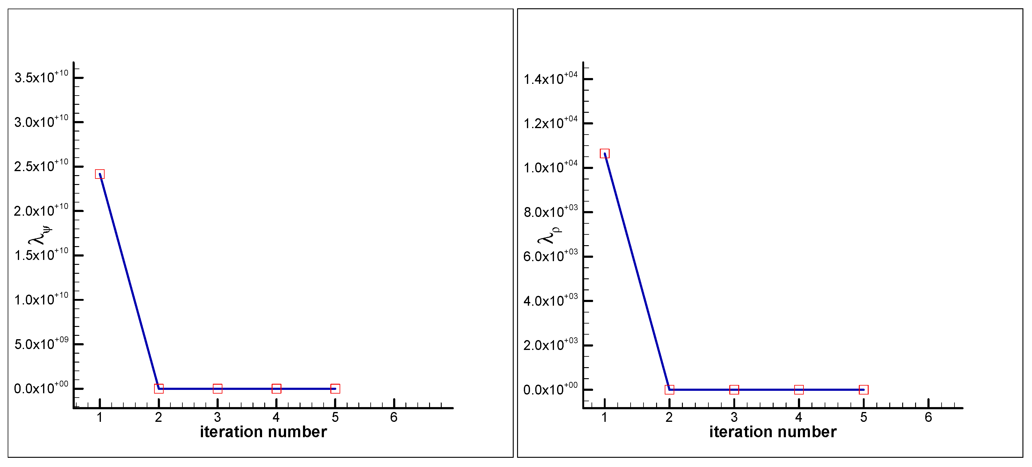
Test case 6: The airfoil surface pressure coefficient distribution for NACA 64-012airfoil and $M_{\infty }=0.3$, $\alpha =6^{\circ }$. The mesh size used in FOILcom is $50\times 141$. The computation time is 46 s. The results from two codes FOILcom and FOILincom along with the Karman-Tsien compressibility correction are compared and depicted in Figure 21. Moreover, the convergence history of ${\lambda }_{\psi }$ and ${\lambda }_{\rho }$ are shown in Figure 22. As can be seen, in this test case five iterations are needed to satisfy the stopping criteria (${\lambda }_{\psi }={\lambda }_{\rho }={10}^{-4}$).

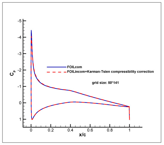
Figure 21. Comparison of surface pressure coefficient distributions for NACA 64-012 airfoil ($M_{\infty }=0.3$, $\alpha =6^{\circ }$) using the codes FOILcom and FOILincom along with the Karman-Tsien compressibility correction.

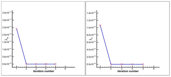
Figure 22. Convergence history of ${\lambda }_{\psi }$ and ${\lambda }_{\rho }$.

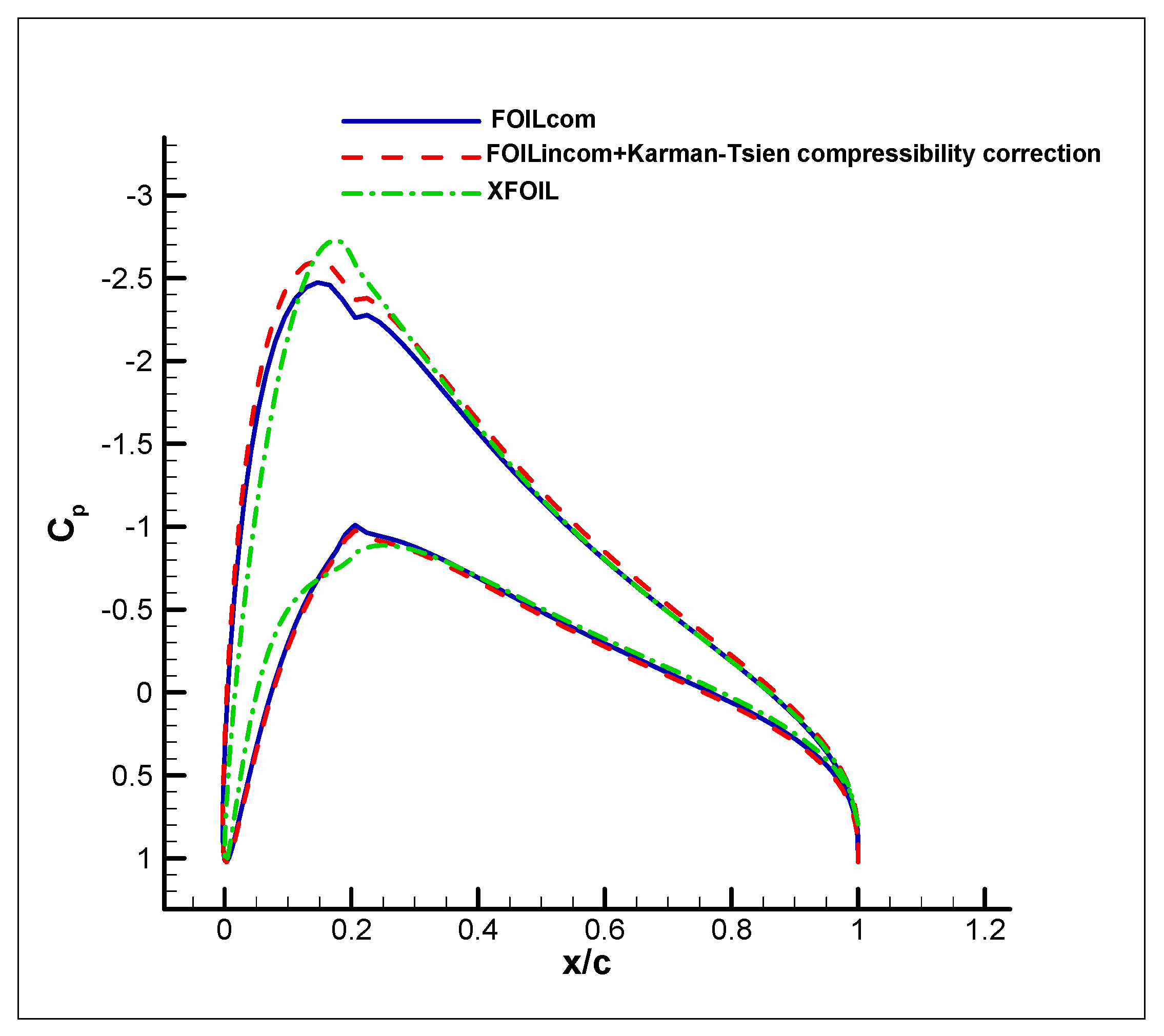
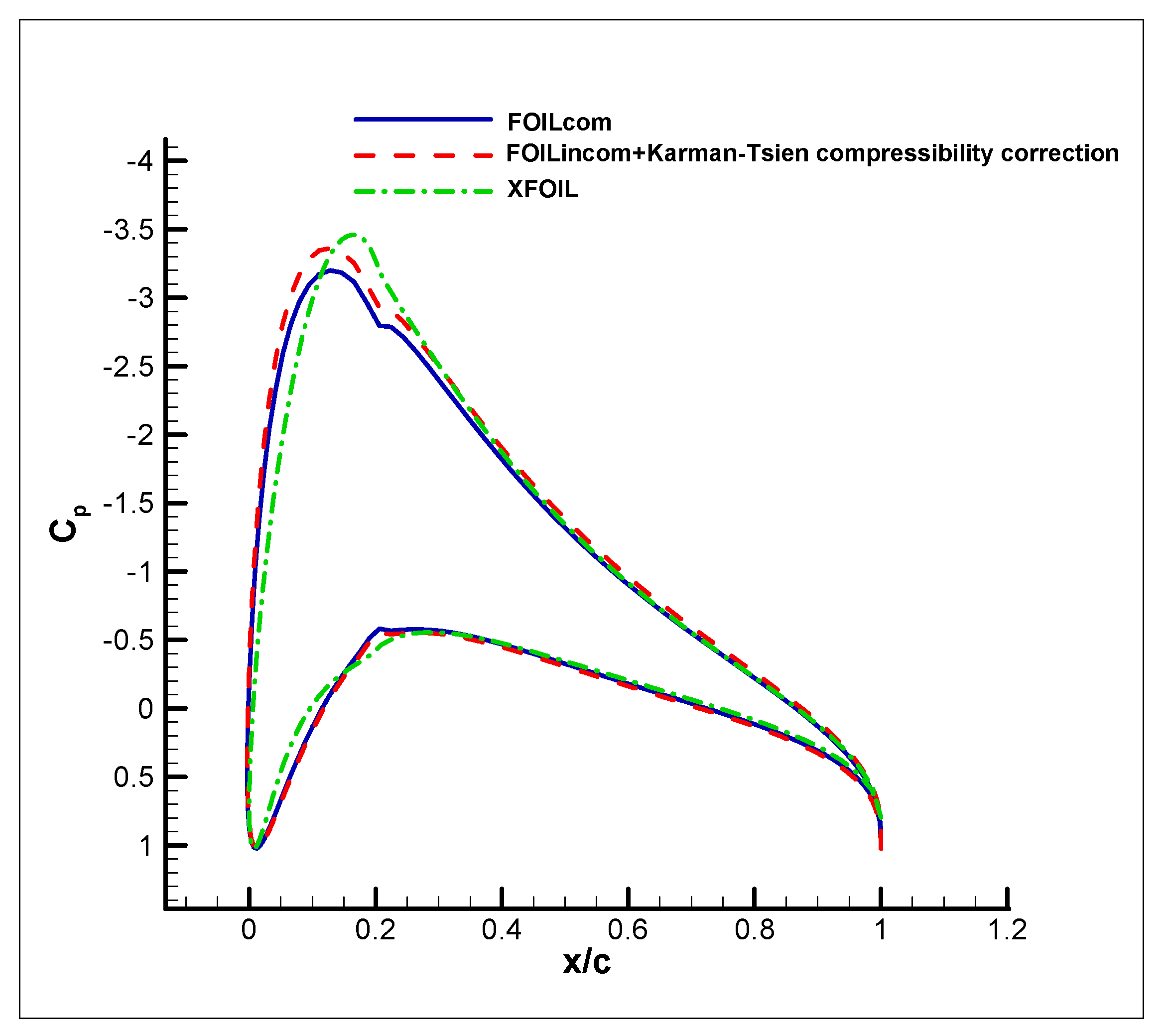
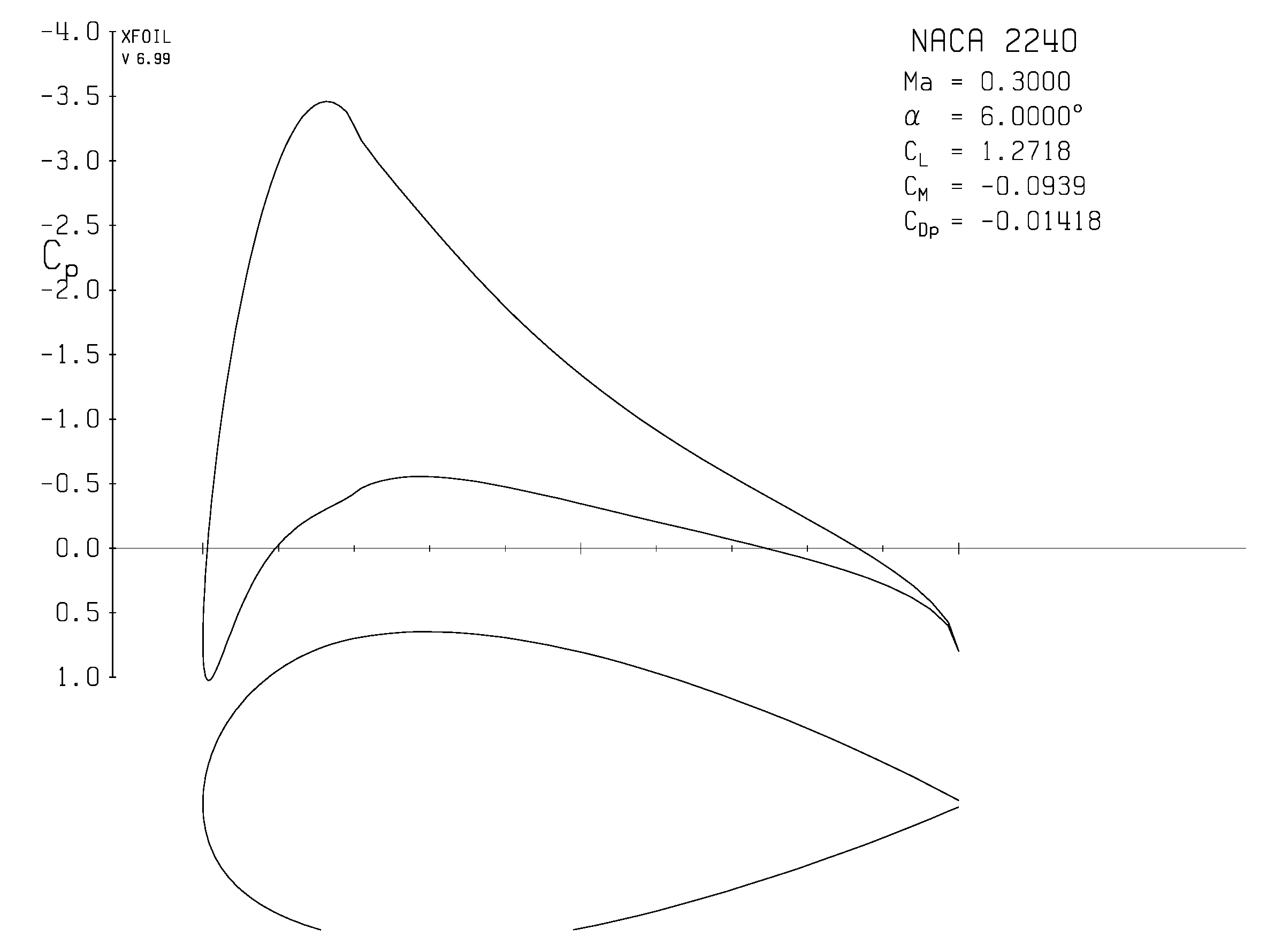
Test case 7: The airfoil surface pressure coefficient distribution for NACA 2240 airfoil and $M_{\infty }=0.3$ at two different angles of attack $\alpha =3^{\circ }$ and $\alpha =6^{\circ }$. The mesh size used in FOILcom is $120\times 141$. In this test case, a thick airfoil, NACA 2240, is used to reveal the accuracy of the proposed numerical method in dealing with thick airfoils at high angles of attack. The results from FOILcom, FOILincom along with the Karman-Tsien compressibility correction, and XFOIL are compared and depicted in Figure 23 for the angle of attack $\alpha =3^{\circ }$ and Figure 24 for the angle of attack $\alpha =6^{\circ }$. Furthermore, the results from XFOIL are given in Figure 25 for the angle of attack $\alpha =3^{\circ }$ and Figure 26 for the angle of attack $\alpha =6^{\circ }$. The drag and lift coefficients using both codes for two different angles of attack are given in Table 2.

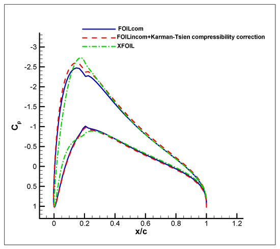
Figure 23. Comparison of surface pressure coefficient distributions for NACA 2240 airfoil ($M_{\infty }=0.3$, $\alpha =3^{\circ }$) using the codes FOILcom, FOILincom along with the Karman-Tsien compressibility correction, and XFOIL.

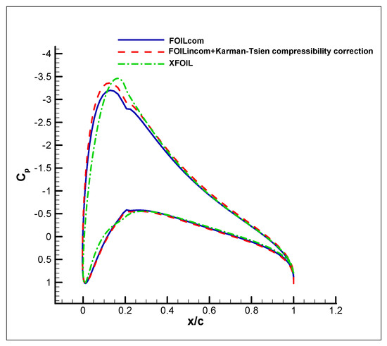
Figure 24. Comparison of surface pressure coefficient distributions for NACA 2240 airfoil ($M_{\infty }=0.3$, $\alpha =6^{\circ }$) using the codes FOILcom, FOILincom along with the Karman-Tsien compressibility correction, and XFOIL.

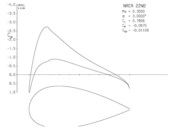
Figure 25. The airfoil surface pressure coefficient distribution for NACA 2240 airfoil ($M_{\infty }=0.3$, $\alpha =3^{\circ }$) using XFOIL.

Figure 26. The airfoil surface pressure coefficient distribution for NACA 2240 airfoil ($M_{\infty }=0.3$, $\alpha =6^{\circ }$) using XFOIL.

Table 2. Drag and lift coefficients using FOILcom and XFOIL.

NACA 2240 Airfoil	${\mathit{c}}_{\mathit{d}}$	${\mathit{c}}_{\mathit{l}}$
$M_{\infty }=0.3$, $\alpha =3^{\circ }$	FOILcom: −0.01668 XFOIL: −0.01126	FOILcom: 0.7977 XFOIL: 0.7806
$M_{\infty }=0.3$, $\alpha =6^{\circ }$	FOILcom: −0.02684 XFOIL: −0.01418	FOILcom: 1.2714 XFOIL: 1.2718

4. Conclusions

The solution of 2D steady, irrotational, subsonic (subcritical) compressible flow over isolated airfoils using the stream function equation and a novel method to implement the Kutta condition have been presented. The numerical scheme takes advantage of transformation of the flow solver and the boundary conditions from the physical domain to the computational domain. The physical domain was meshed by an O-grid elliptic grid generation method and the transformed flow solver is discretized by finite-difference method, a method chosen for its simplicity and ease of implementation. The numerical scheme is exempt from considering the panels and the quantities such as the vortex panel strength and circulation used in the panel method. An accurate Kutta condition scheme is proposed and implemented into the computational loop by an exact derived expression for the stream function at the airfoil trailing edge. The exact expression is general, and encompasses both the finite-angle and cusped trailing edges. Through several test cases, the proposed numerical scheme was validated by results from the experimental and the other numerical methods. The obtained results revealed that the proposed algorithm is very accurate and robust.

References

- Hess, J.L.; Smith, A.M.O. Calculation of potential flow about arbitrary bodies. Prog. Aerosp. Sci. 1967, 8, 1–138. [Google Scholar] [CrossRef]
- Hess, J. Panel methods in computational fluid dynamics. Annu. Rev. Fluid Mech. 1990, 22, 255–274. [Google Scholar] [CrossRef]
- Erickson, L.L. Panel Methods: An Introduction; NASA Ames Research Center: Moffett Field, CA, USA, 1990. [Google Scholar]
- Anderson, J.D. Fundamentals of Aerodynamics; McGraw-Hill Education: New York, NY, USA, 2016. [Google Scholar]
- Drela, M. Flight Vehicle Aerodynamics; MIT Press: Cambridge, MA, USA, 2014. [Google Scholar]
- Katz, J.; Plotkin, A. Low-Speed Aerodynamics; Cambridge University Press: Cambridge, UK, 2001. [Google Scholar]
- Kutta, W.M. Lifting Forces in Flowing Fluids; G. Braunbeck & Gutenberg: Berlin, Germany, 1902. [Google Scholar]
- Lewis, R.I. Vortex Element Methods for Fluid Dynamic Analysis of Engineering Systems; Cambridge University Press: Cambridge, UK, 1991. [Google Scholar]
- Xu, C. Kutta Condition for sharp edge flows. Mech. Res. Commun. 1998, 25, 415–420. [Google Scholar] [CrossRef]
- Jacob, K.; Riegels, F. The calculation of the pressure distribution over aerofoil sections of finite thickness with and without flaps and slats. Z. Flugwiss 1963, 11, 357–367. [Google Scholar]
- Drela, M. XFOIL: An analysis and design system for low Reynolds number airfoils. InLow Reynolds Number Aerodynamics; Springer: Berlin/Heidelberg, Germany, 1989; pp. 1–12. [Google Scholar]
- Cummings, R.M.; Mason, W.H.; Morton, S.A.; McDaniel, D.R. Applied Computational Aerodynamics: A Modern Engineering Approach; Cambridge University Press: Cambridge, UK, 2015. [Google Scholar]
- Hirsch, C. Numerical Computation of Internal and External Flows, Computational Methods for Inviscid and Viscous Flows; Wiley: Chichester, UK, 1991. [Google Scholar]
- Shapiro, A.H. The Dynamics and Thermodynamics of Compressible Fluid Flow; John Wiley & Sons: New York, NY, USA, 1953. [Google Scholar]
- Yahya, S.M. Fundamentals of Compressible Flow: SI Units with Aircraft and Rocket Propulsion; New Age International: Delhi, India, 2003. [Google Scholar]
- Johnson, R.W. Handbook of Fluid Dynamics; CRC Press: Boca Raton, FL, USA, 2016. [Google Scholar]
- Mohebbi, F. Optimal Shape Design based on Body-Fitted Grid Generation; University of Canterbury: Christchurch, New Zealand, 2014. [Google Scholar]
- Thompson, J.; Warsi, Z.; Mastin, C. Numerical Grid Generation: Foundations and Applications. 1997. Available online: https://www.hpc.msstate.edu/publications/gridbook/PDFS/NumericalGridGenerationComplete.pdf (accessed on 25 June 2019).
- Özişik, M.N.; Orlande, H.R.B.; Colaço, M.J.; Cotta, R.M. Finite Difference Methods in Heat Transfer; CRC Press: Boca Raton, FL, USA, 2017. [Google Scholar]
- Thames, F.C.; Thompson, J.F.; Mastin, C.W. Numerical Solution of the Navier-Stokes Equations for Arbitrary Two-Dimensional Airfoils; Mississippi State Univiversity: Mississippi State, MS, USA, 1975. [Google Scholar]
- Mohebbi, F.; Sellier, M. On the Kutta condition in potential flow over airfoil. J. Aerodyn. 2014, 2014, 676912. [Google Scholar] [CrossRef]
- Freuler, R.; Gregorek, G. An Evaluation of Four Single Element Airfoil Analytic Methods; Ohio State University, General Aviation Airfoil Design and Analysis Center: Columbus, OH, USA, 1979. [Google Scholar]
- Katz, A.; Jameson, A. Meshless scheme based on alignment constraints. AIAA J. 2010, 48, 2501–2511. [Google Scholar] [CrossRef]
- Jameson, A.; Caughey, D.; Jou, W.; Steinhoff, J.; Pelz, R. Accelerated finite-volume calculation of transonic potential flows. In Numerical Methods for the Computation of Inviscid Transonic Flows with Shock Waves; Springer: Braunschweig, Germany, 1981; pp. 11–27. [Google Scholar]
© 2019 by the authors. Licensee MDPI, Basel, Switzerland. This article is an open access article distributed under the terms and conditions of the Creative Commons Attribution (CC BY) license (http://creativecommons.org/licenses/by/4.0/).