On Solving the Nonlinear Falkner–Skan Boundary-Value Problem: A Review

Abstract

This article is a review of ongoing research on analytical, numerical, and mixed methods for the solution of the third-order nonlinear Falkner–Skan boundary-value problem, which models the non-dimensional velocity distribution in the laminar boundary layer.

1. Introduction

The Falkner–Skan equation, a third-order ordinary differential equation over a semi-infinite domain, was originally developed in 1931 by Falkner and Skan [1] from a similarity analysis on the steady, two-dimensional, boundary-layer flow of an incompressible, viscous fluid over a wedge [2]. As it turns out, the solution of the Falkner–Skan equation represents the laminar boundary layer over an infinite wedge whose vertex angle is $\beta \pi$ for $0\le \beta \le 2$, as illustrated in Figure 1.

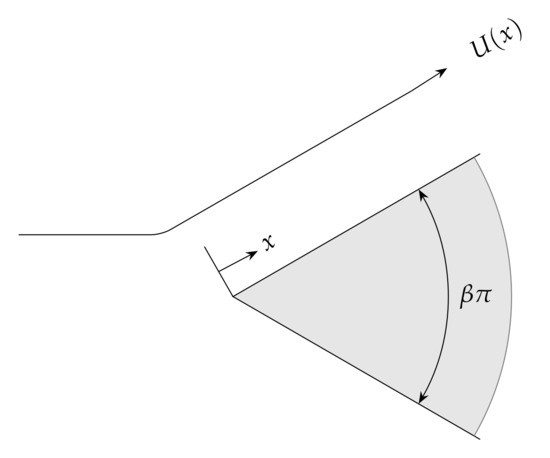
Figure 1. Boundary layer flow past a wedge.

The case $\beta =0$ corresponds to the flow past a flat plate and leads to the well-known Blasius equation [3], and the case $\beta =1$ corresponds to what is known as the stagnation-point flow or the Hiemenz flow [4]. The similarity analysis begins with the continuity and the momentum equations that are described by

$$\begin{array}{cc}\hfill \frac{\partial u}{\partial x}+\frac{\partial v}{\partial y}& =0,\hfill \end{array}$$

(1)

$$\begin{array}{cc}\hfill u\frac{\partial u}{\partial x}+v\frac{\partial u}{\partial y}& =U\frac{dU}{dx}+\mu \frac{{\partial }^{2}u}{\partial y^2},\hfill \end{array}$$

(2)

subject to the boundary conditions

$$u(x,0)=v(x,0)=0,\mathrm{and}u(x,y)\to U\left(x\right)\mathrm{as}y\to \infty .$$

(3)

In (1)–(3), u and v are the velocity components in the x and y directions of the fluid flow; $\mu$ is the viscosity; and $U\left(x\right)$ is the velocity at the end of the boundary layer. A stream function $\mathsf{\Psi }(x,y)$ is defined so that the continuity Equation (1) is automatically satisfied. Accordingly, it must be true that

$$u=\frac{\partial \mathsf{\Psi }}{\partial y},\mathrm{and}v=-\frac{\partial \mathsf{\Psi }}{\partial x}.$$

Falkner and Skan [1] proposed the transformations

$$\eta =\left(\sqrt{\frac{U\left(x\right)}{\mu x}}\right)y,\mathrm{and}f\left(\eta \right)=\frac{\mathsf{\Psi }(x,y)}{\sqrt{U\left(x\right)\mu x}}.$$

(4)

With the assumption that $U\left(x\right)$ satisfies the power law $U\left(x\right)=c{x}^m$ for some constant c and $m=\frac{\beta }{2-\beta }$, under the transformations (4), the momentum Equation (2) becomes

$$f^{‴}+f{f}^{″}+\beta \left(1-{\left(f^{\prime }\right)}^2\right)=0,$$

(5)

subject to the boundary conditions

$$f\left(0\right)=f^{\prime }\left(0\right)=0,\mathrm{and}{f}^{\prime }\left(\eta \right)\to 1\mathrm{as}\eta \to \infty .$$

(6)

derived from the corresponding transformation of (3). In (5) and (6), the primes denote differentiation with respect to $\eta$. The nonlinear, third-order, ordinary differential Equation (5) is known as the Falkner–Skan equation. Together, (5) and (6) will be referred to as the Falkner–Skan boundary-value problem. Solutions of (5) and (6) are characterized by the numerical value $\alpha =f^{″}\left(0\right)$.

Many industrial processes such as the drawing of plastic films, metal spinning, cooling of a metallic plate, and aerodynamic extrusion of plastic sheets require the solution of the Falkner–Skan equation and several of its variants applied to different geometries and corresponding boundary conditions [5]. Thus, there has been a considerable research interest in solving the Falkner–Skan equation during the past few decades. Analytical investigations of this problem have been aimed at providing existence and uniqueness results, finding exact, nearly-exact, or approximate analytical solutions. Computational approaches include a spectrum of methods ranging from the traditional finite-difference and finite-element methods to applying neural networks. The purpose of this review article is to provide a succinct summary of these various approaches that have been used for solving this important nonlinear boundary-value problem.

2. Materials and Methods

For the purpose of this review, we will be specifically investigating the problem as posed by (5) and (6). As this is a review article focused on the existing literature, this section will be devoted to describing the methods and/or approaches used by previous researchers. Accordingly, this section will include two main subsections, the first one reviewing analytical treatments, and the second exploring the computational approaches documented thus far in the literature. The discussion of analytical treatments will include existence and uniqueness results, exact or nearly-exact analytical solutions, and approximate analytical solutions. The discussion of computational approaches will include the description of the different classes of methods currently available.

2.1. Analytical Treatments

The first result on the existence and uniqueness of a solution to (5) and (6), with the additional assumption of $f^{\prime }>0$, is due to Weyl [6] and this result was proved using a fixed-point theorem. Later, Coppel [7] assumed $0<f^{\prime }<1$, considered three-dimensional trajectories in the phase-space, and established the existence and uniqueness result of Weyl [6], along with many more details on the asymptotic behavior of the solutions with $\beta \ge 0$ for various scenarios related to $\beta$ in (5). In addition, Coppel [7] also showed that $\alpha =f^{″}\left(0\right)$ is an increasing function of $\beta$. Tam [8] removed Coppel’s assumption of $0<f^{\prime }<1$ and established the existence and uniqueness result using a shooting argument. Craven et al. [9] proved the existence and uniqueness of solutions for $0\le \beta <1$ by arguing that in this range, the condition $0<f^{\prime }<1$ is satisfied. Solutions of (5) and (6) which have $f^{\prime }\left(\eta \right)<0$ for $\eta >0$ represent what are known as reverse flows. Stewartson [10] was the first to obtain reverse flows for $\beta \in (-0.1988,0)$. The existence and uniqueness of the reverse flows obtained by Stewartson was proved by Hastings [11]. In related work, Craven et al. [12] carried out numerical experiments that suggested the existence of reverse flows for $\beta >1$. Other works on existence and uniqueness of solutions to (5) and (6) may also be found in Rosenhead et al. [13] and Hartman [14]. Veldman and Van der Vooren [15] have extended Coppel’s work for $\beta <0$. The work of Oskam et al. [16] is also focused on the study of (5) for $\beta <0$. In place of the boundary conditions in (6), Oskam et al. [16] consider two scenarios, one corresponding to $f^{\prime }(\infty )=1$, and one corresponding to $f^{\prime }(\infty )=-1$, which are closely related as $\beta \to 0^{-}$. Moreover, for $\beta <-1$, these two scenarios allow multiple solutions which are characterized and distinguished using the number of zeros of $f^{\prime }-1$. Additionally, for $\beta <-1$, this work provides a periodic solution as well, and a more general treatment of periodic solutions is presented by Botta et al. [17]. Rajagopal et al. [18] have established non-similar solutions for the boundary layer flow of a homogeneous incompressible fluid of second grade past a wedge placed symmetrically with respect to the flow direction and discussed the variation of the skin-friction with respect to the non-Newtonian parameters. In particular, by expressing the solution as a power series in terms of a parameter $\epsilon$ that scales velocities with the square root of the Reynolds number, they obtain the zeroth-order and first-order solutions. Their zeroth-order solution coincides with the classical Falkner–Skan flow which we have explored in this review. They have numerically computed the second-order solution and analyzed it more in-depth as it relates to variations in the parameter $\epsilon$. Massoudi et al. [19] have investigated the effects of the non-Newtonian nature of a fluid on the shear stress at the wall as well as the velocity profiles for different injection and suction rates and different values of the wedge angle $\beta$. Additional existence and uniqueness results for the solution of the Falkner–Skan equations are also given by Padé [20].

More generally, with (5) written in the form

$$f^{‴}+{\beta }_{0}f{f}^{″}+\beta (1-{\left(f^{\prime }\right)}^2)=0,$$

(7)

subject to the boundary conditions (6), several instances corresponding to specific choices of values for ${\beta }_0$ and $\beta$ have been explored analytically.

2.1.1. The Pohlhausen Flow

For $({\beta }_0,\beta )=(0,1)$, (7) leads to what is known as the Pohlhausen flow [21]. This instance, described by

$$f^{‴}+(1-{\left(f^{\prime }\right)}^2)=0$$

(8)

has the exact solution given by

$$f^{\prime }\left(\eta \right)=3{tanh}^2\left[\frac{\eta }{\sqrt{2}}+{tanh}^{-1}\sqrt{\frac{2}{3}}\right]-2.$$

(9)

It is sometimes used to validate numerical methods [22].

2.1.2. The Blasius Flow

With $({\beta }_0,\beta )=(\frac{1}{2},0)$ (7) takes the form

$$f^{‴}+\frac{1}{2}f{f}^{″}=0$$

(10)

and leads to the well-known Blasius probem [3]. While a closed-form solution is not available for (10), it has been subject to extensive analytical treatment as well as numerical investigation. We briefly describe some selected analytical treatments here and postpone the discussion of the numerical investigations to a later section.

For the case of (10), Blasius [3] proposed the power series solution

$$f\left(\eta \right)=\sum _{k=0}^{\infty }{\left(-\frac{1}{2}\right)}^k\frac{A^k{\alpha }^{k+1}}{(3k+2)!}{\eta }^{3k+2},$$

(11)

with

$$A_k=\left\{\begin{array}{cc}1,\hfill & \mathrm{for}k=0,1;\hfill \\ {\displaystyle \sum _{r=0}^{k-1}\left({\displaystyle \genfrac{}{}{0pt}{}{3k-1}{3r}}\right)A_r{A}_{k-r-1},}\hfill & \mathrm{for}k\ge 2,\hfill \end{array}\right.$$

(12)

and $\alpha =f^{″}\left(0\right)$. This solution requires knowledge of $\alpha =f^{″}\left(0\right)$ and, several works [23,24] have pointed out that the above series is valid only for small values of $\eta$. As the search for an approximate analytical solution of (10) continued, Ahmad and Al-Barakati [25] modified the [4/3] Padé approximant for the derivative to satisfy its asymptotic behavior and obtained the solution

$$f^{\prime }\left(\eta \right)\approx \frac{0.332057\eta +0.00059069{\eta }^4+0.00000288{\eta }^{5}exp({\eta }^2/4-1)}{1+0.0086967{\eta }^3+0.00000288{\eta }^{5}exp({\eta }^2/4-1)}.$$

(13)

Beginning with an approximate solution of the form $f\left(\eta \right)=1/(A\eta +B)$ that contains the undetermined coefficients A and B, Bougoffa and Wazwaz [26] use the differential Equation (10) and the boundary conditions (6) to obtain the approximate analytical solution

$$f\left(\eta \right)=\eta -6+\frac{36}{\eta +6}.$$

(14)

Other works that provide asymptotic approximants to the solution of (5) and (6) include Belden et al. [27].

2.1.3. The Crocco–Wang Transformation

Another interesting line of investigation of the Falkner–Skan and Blasius flows has evolved due to the suggestion of the transformation

$$x=f^{\prime }\left(\eta \right),y=f^{″}\left(\eta \right),$$

(15)

that originally appeared in Crocco [28], and later independently used by Wang [29]. Under the transformation (15), the third-order boundary-value problem (10) along with the boundary conditions (6) on the semi-infinite domain $[0,\infty )$ takes the form

$$2y{y}^{″}+x=0,y^{\prime }\left(0\right)=0,\mathrm{and}y\left(1\right)=0,$$

(16)

which is a second-order boundary-value problem on a finite interval. Note that in (16) the primes denote differentiation with respect to the variable x. In this form, the quantity $y(x=0)$ corresponds to $\alpha =f^{″}(\eta =0)$ that characterizes the solution of the Blasius problem. Brighi et al. [30] provides a historical review of the research on the Blasius problem. Several analytical approaches to analyzing and solving (16) are currently available. The work of Varin [31], where $y(x=0)$ is referred to as the Blasius constant, examines the Crocco Equation (16) and provides the following results: (1) The non-existence of singularities other than the $x=1$ in (16) (which represents $\eta \to \infty$ in (6)); (2) an explicit expression for the Blasius constant as a sum of a series of rational numbers; (3) a recursive formula for the coefficients of the series; and (4) a numerical procedure for computing the Blasius constant to high accuracy.

Under the Crocco–Wang transformation (15), the Falkner–Skan problem (5) and (6) becomes

$$y^{″}+\left({\beta }_0-2\beta \right)\frac{x}{y}-\beta \left(\frac{1-x^2}{y^2}\right)y^{\prime }=0,y^{\prime }\left(0\right)=-\frac{\beta }{y\left(0\right)},\mathrm{and}y\left(1\right)=0,$$

(17)

in which the primes denote differentiation with respect to the variable x. Note that $y(x=0)$ corresponds to $\alpha =f^{″}(\eta =0)$ also for the transformed Falkner–Skan equation as it did for the Blasius equation. The existence of a unique positive solution to a variant of the instance of (17) corresponding to the Homann [32] flow, or $({\beta }_0,\beta )=(1,\frac{1}{2})$, has been demonstrated in Shin [33].

2.1.4. Other More General Analytical Approaches

Adomian Decomposition Method (ADM). Rewriting (5) as $(L+N)f=0$ where $Lf=f^{‴}$ and $Nf=f{f}^{″}+\beta (1-{\left(f^{\prime }\right)}^2)$, ADM proceeds to obtain $f\left(\eta \right)$ as an infinite series of the form ${\sum }_{n=0}^{\infty }{f}_n\left(\eta \right)$. First, $f_0\left(\eta \right)$ in the infinite series expansion is obtained as the solution of the homogeneous equation $L{f}_0=0$, which yields

$$f_0\left(\eta \right)=\alpha \frac{{\eta }^2}{2}-\beta \frac{{\eta }^3}{6}.$$

In order to obtain $f_n\left(\eta \right)$, the ADM defines the Adomian polynomials as

$$A_n=\frac{1}{n!}\frac{d^n}{d{\lambda }^n}{\left[N\left(\sum _{j=0}^n{\lambda }^j{f}_j\left(\eta \right)\right)\right]}_{\lambda =0},$$

(18)

and sets

$$f_{n+1}\left(\eta \right)=L^{-1}\left(A_n\right),n=0,1,2,\cdots .$$

(19)

According to Alizadeh et al. [34], the ADM is more realistic compared to other methods that may use linearization in some form or another, or assume some weak nonlinearity, or simplify the physical problem. On the other hand, the ADM involves a considerable amount of symbolic manipulation in order to obtain more terms in the infinite series expansion. For the Falkner–Skan problem, the results reported in [34] indicate that ADM required from 2 to 30 terms in the infinite series expansion as the wedge angle was varied from $0^{\circ }$ (flat plate) to ${180}^{\circ }$ (stagnation flow).

Homotopy Methods. A variety of methods, known by the names of Homotopy Asymptotic Method (HAM) [35], Optimal Homotopy Asymptotic Method (OAHM) [36,37,38], and Homotopy Perturbation Method (HPM) [39,40] have also been used to obtain approximate analytical solutions to the Falkner–Skan problem (5) and (6). These methods express the problem in the form

$$(1-p)L\left(\varphi \right(\eta \left)\right)+pN\left(\varphi \right(\eta \left)\right)=0$$

(20)

where L is an easily invertible linear part of the operator representing the Falkner–Skan problem, N the entire nonlinear operator that represents the Falkner–Skan equation, and p a parameter that varies from 0 to 1. The form (20) is set up such that the solution corresponding to $p=0$ can be easily obtained by inverting the linear operator, and the solution corresponding to $p=1$ is the desired solution of the Falkner–Skan problem, both satisfying the boundary conditions (6). In order to advance the solution from $p=0$ to $p=1$, the desired solution is assumed to be of the form

$$f\left(\eta \right)=f_0\left(\eta \right)+\sum _{k=1}^{\infty }{f}_k\left(\eta \right)p^k.$$

(21)

Beginning with $f_0\left(\eta \right)$ obtained as the solution of $L\varphi \left(\eta \right)=0$ subject to the boundary conditions (6), plugging the form (21) into (20), differentiating with respect to p as many times as desired and setting $p=0$ yields a succession of equations to solve for $f_k\left(\eta \right)$. An efficient implementation of HAM by the name Spectral HAM (SHAM) [41] has also been proposed, and this method obtains the initial solution using collocation at Chebyshev points after suitably transforming the semi-infinite domain into the interval $[-1,1]$. It is customary to call p the embedding parameter. In addition to p, the HAM approach allows for the use of another parameter h known as the convergence control parameter.

As evident from the above discussion, most studies focused on the analytical treatment of (5) and (6) or its variants have demonstrated a solution’s existence and uniqueness, developed semi-analytic, asymptotic solutions for special cases, or discovered ranges of validity for the boundary-layer parameters and similarity variables [5,6,8,13,14,20,42]. However, a general closed-form solution is still unavailable for this two-point boundary-value problem in spite of the efforts dedicated to its investigation. Therefore, approaching its solution numerically has been the most common and valuable route.

2.2. Numerical Treatments

Several different numerical approaches have been used to investigating the Falkner -Skan problem (5) and (6), and they are in the categories of shooting, finite-differences, collocation, and other methods. The first computational treatment reported in the literature is due to Hartree [43]. While the details of the numerical approach are not provided in this work, Hartree [43] showed that physically relevant solutions of (5) and (6) exist only in the range ${\displaystyle -0.198838\le \beta \le 4/3}$. Smith [44], Cebeci and Keller [45], and Na [46] have used shooting and invariant imbedding to solve the Falkner–Skan problem directly on the semi-infinite domain. The methods that came about after these early treatments mainly focused on making the computational methods more efficient and/or skillfully dealing with the boundary condition at infinity. Various special cases of (5) and (6) have been used to validate the effectiveness of the methods developed.

Coordinate transformations and appropriate change of variables have been used for the purpose of mapping the physical domain $[0,\infty )$ to a computational domain like $[0,1]$ or $[-1,1]$. It is also common practice to truncate the physical domain where $\eta \to \infty$ by a finite value $\eta ={\eta }_{\infty }$ which is determined as part of the solution, and impose the boundary condition as $\eta \to \infty$ at the truncated boundary $\eta ={\eta }_{\infty }$. Once transformed to a suitable computational form, methods vary depending on the specific way in which numerical computations are carried out. Among the different techniques used for this purpose are, shooting; finite-differences; and collocation methods. Along with these fundamental differences in the approach, the methods also vary based on the specific techniques used for the computational problems that result. In this section, we will review these approaches and the associated computational techniques.

2.2.1. Shooting

The term shooting in numerical analysis refers to the idea of solving a two-point boundary-value problem iteratively by repeatedly solving an initial-value problem aimed at obtaining the value

$$\frac{d^{2}f}{d{\eta }^2}=\alpha ,\mathrm{at}\eta =0$$

(22)

such that the boundary condition as $\eta \to \infty$ is satisfied. With an initial guess for $\alpha$, the shooting process involves marching the solution from $\eta =0$ to $\eta =\infty$, and adjusting or improving the guess for the value of $\alpha$ appropriately so that the boundary condition at $\eta =\infty$ is satisfied. There are several ways in which the methods that employ the shooting approach may differ. These include the initial guess for $\alpha$, the choice of the method that advances the solution from $\eta =0$ to $\eta =\infty$, and the manner in which the guess for $\alpha$ is adjusted.

As mentioned earlier, the semi-infinite physical domain $[0,\infty )$ is first mapped to a finite computational domain like $[0,1]$ using an appropriate coordinate transformation. For this purpose, a finite boundary $\eta ={\eta }_{\infty }$ is first introduced and the value of ${\eta }_{\infty }$ will be determined as part of the solution. It is customary to introduce the “asymptotic condition” $\frac{d^{2}f}{d{\eta }^2}=0$ as $\eta \to \infty$ to help determine the additional unknown ${\eta }_{\infty }$. Thus, with the truncated domain $[0,{\eta }_{\infty }]$, the conditions

$$\frac{df}{d\eta }=1,\frac{d^{2}f}{d{\eta }^2}=0\mathrm{at}\eta ={\eta }_{\infty }$$

(23)

will be imposed. Next, we observe that under the coordinate transformation $\xi =\eta /{\eta }_{\infty }$ [47], the problem (5) and (6) becomes

$$\frac{1}{{{\eta }_{\infty }}^3}\frac{d^{3}f}{d{\xi }^3}+\frac{1}{{{\eta }_{\infty }}^2}f\frac{d^{2}f}{d{\xi }^2}+\beta \left[1-\frac{1}{{{\eta }_{\infty }}^2}{\left(\frac{df}{d\xi }\right)}^2\right]=0,$$

(24)

subject to the boundary conditions

$$\begin{array}{cccc}\hfill f\left(\xi \right)& =0,\mathrm{at}\xi \hfill & & =0,\hfill \end{array}$$

(25)

$$\begin{array}{cccc}\hfill \frac{1}{{\eta }_{\infty }}\frac{df}{d\xi }& =0,\mathrm{at}\xi \hfill & & =0,\hfill \end{array}$$

(26)

$$\begin{array}{cccc}\hfill \frac{1}{{\eta }_{\infty }}\frac{df}{d\xi }& =1,\mathrm{at}\xi \hfill & & =1.\hfill \end{array}$$

(27)

At this point, applying the the change of variables

$$u=\frac{1}{{\eta }_{\infty }}\frac{df}{d\xi },v=\frac{1}{{\eta }_{\infty }^2}\frac{d^{2}f}{d{\xi }^2}$$

(28)

transforms the single third-order differential equation to (24) to the system of three first-order differential equations

$$\frac{df}{d\xi }={\eta }_{\infty }u,\frac{du}{d\xi }={\eta }_{\infty }v,\frac{dv}{d\xi }=-{\eta }_{\infty }(fv+\beta (1-u^2),$$

(29)

while the boundary conditions (25), (26) and (22) become

$$f=0,u=0,\mathrm{and}v=\alpha ,\mathrm{at}\xi =0,$$

(30)

Additionally, the conditions (23) now take the form

$$u=1\mathrm{and}v=0\mathrm{at}\xi =1.$$

(31)

Note that (29) and (30) together represent an initial value problem. With the correct value of $\alpha$, the initial value problem (29) and (30) should produce u and v that satisfy the conditions (31). Conversely, in order to obtain the correct value for $\alpha$, the initial value problem (29) and (30) is first solved with an initial guess for $\alpha$ in (29), the values of the u and v at $\xi =1$ based on this solution are used to improve upon the guess for $\alpha$. This process is repeated until the conditions (31) are satisfied. The following is a listing of the works that have used the shooting approach along with a description of how they differed from the others using the same approach:

• The work of Cebeci and Keller [45] is the first to employ the shooting approach to solve (5) and (6). They work directly with the physical domain $\eta \in [0,\infty )$, but march their solution from $\eta =0$ to $\eta ={\eta }_{\infty }$, where they assume ${\eta }_{\infty }$ is “sufficiently large.” They use the Newton’s method to adjust the initial condition.
• Cebeci and Keller [45] also employ the idea of parallel shooting to obtain the solution. This approach involves dividing the domain into several subintervals and applying shooting in each subinterval. The motivation for this approach comes from the desire to avoid any instabilities that may be caused while marching the solution using an initial-value method. The authors report successfully obtaining three significant digits in two iterations when shooting was carried out over three subintervals.
• Asaithambi [47] uses the classical, fourth-order Runge-Kutta method to march the solution from $\xi =0$ to $\xi =1$ and the secant method to iteratively obtain improved values for $\alpha$. Two initial approximations for $\alpha$ were needed.
• Salama [48] uses a single-step method of order 5 to march the solution from $\xi =0$ to $\xi =1$, coupled with a third-order rootfinding method called the Halley’s method [49] to compute $\alpha$ and the secant method to compute ${\eta }_{\infty }$. It is also important to note that the solutions of (5) and (6) are obtained for $\beta$ values as large as 40.
• In another work, Asaithambi [22] uses recursive evaluation of Taylor coefficients to march the solution from $\xi =0$ to $\xi =1$ and the secant method to iteratively obtain improved values for $\alpha$. Two initial approximations for $\alpha$ were needed, and higher orders of accuracy, as high as 7, were achieved with ease. Moreover, this work explores (5) and (6) for $\beta$ values as large as 40 as well and compares the results obtained previously by Salama [48].
• Zhang and Chen [50] used the Runge-Kutta (4,5) formula to march the solution from $\xi =0$ to $\xi =1$, and the Newton’s method to improve the guess for $\alpha$, and hence required only one initial guess to get started.
• Sher and Yakhot [51] shoot from the end corresponding to $\eta \to \infty$ instead of from $\eta =0$. They choose an arbitrary value for $f\left(\eta \right)$ as $\eta \to \infty$, a value close to 1 for $f^{\prime }\left(\eta \right)$ as $\eta \to \infty$ and estimate $f^{″}\left(\eta \right)$ as $\eta \to \infty$ using a simple analysis of the asymptotic behavior of the solution.

2.2.2. Finite Differences

The finite-difference approach is often used as a more efficient alternative to the shooting approach, as the use of finite differences does not warrant the repeated solution of initial-value problems as does the shooting approach. The following is a listing of the works that have used finite differences, along with a description of how they differed from the others using the same approach:

• Asaithambi [52] truncates the infinite domain at $\eta ={\eta }_{\infty }$, uses the transformation $\xi =\eta /{\eta }_{\infty }$ as done previously, and sets $u=\frac{1}{{\eta }_{\infty }}\frac{df}{d\xi }$, to transform the problem (5) and (6) on the physical domain $\eta \in [0,\infty )$ to the system

  $$\begin{array}{cc}\hfill \frac{df}{d\xi }& ={\eta }_{\infty }u,\hfill \end{array}$$

  (32)

  $$\begin{array}{cc}\hfill \frac{d^{2}f}{d{\xi }^2}& =-{\eta }_{\infty }f\frac{du}{d\xi }-{\eta }_{\infty }^2\beta (1-u^2),\hfill \end{array}$$

  (33)

  on the computational domain $\xi \in [0,1]$, subject to the conditions

  $$\begin{array}{cccccccccc}\hfill f& =0,u\hfill & & =0\hfill & & \mathrm{at}\hfill & & \xi \hfill & & =0,\hfill \end{array}$$

  (34)

  $$\begin{array}{cccccccccc}\hfill u& =1,\frac{du}{d\xi }\hfill & & =0\hfill & & \mathrm{at}\hfill & & \xi \hfill & & =1.\hfill \end{array}$$

  (35)
  In order to discretize (32)–(35), the interval $\xi \in [0,1]$ is subdivided into N subintervals $[{\xi }_j,{\xi }_{j+1}]$ for $j=0,1,\cdots ,N-1$ at ${\xi }_j=jh$ with $h=1/N$. Letting $f_j$ and $u_j$ denote the approximations to $f\left({\xi }_j\right)$ and $u\left({\xi }_j\right)$ respectively, Equation (32) is discretized as

  $$\frac{f_j-f_{j-1}}{h}-{\eta }_{\infty }\left[\frac{u_j+u_{j-1}}{2}\right]=0,j=1,2,\cdots ,N,$$

  (36)

  and Equation (33) is discretized as

  $$\frac{f_{j-1}-2f_j+f_{j+1}}{h^2}+{\eta }_{\infty }{f}_j\frac{u_{j+1}-u_{j-1}}{2h}+{\eta }_{\infty }^2\beta (1-u_j^2)=0,j=1,2,\cdots ,N-1.$$

  (37)
  The boundary conditions (34) translate to

  $$f_0=0,u_0=0,$$

  (38)

  and the conditions (35) translate to

  $$u_N=1,\frac{3u_N-4u_{N-1}+u_{N-2}}{2h}=0.$$

  (39)
  Newton’s method is used for the iterative solution of the nonlinear system (37), Equation (36) is used to update the values of $f_j$, and (39) is used to update ${\eta }_{\infty }$. The solution of the nonlinear system by Newton’s method involves the repeated solution of a linear system with a tridiagonal coefficient matrix. In related work, Asaithambi [53] uses the transformation $\xi =e^{-\eta }$ to map the physical domain $[0,\infty )$ to the computational domain $[0,1]$ and discretizes the transformed equations and boundary conditions using second-order finite differences. This approach does not truncate the physical domain but still requires the iterative solution of a nonlinear system that involves the solution of a tridiagonal linear system during each iteration.
• Salama and Mansour [54] develop an unconditionally stable, fourth order finite difference method that involves only four grid points and apply it to the nonlinear Falkner–Skan problem (5) and (6). Their development uses the method of undetermined coefficients involving the unknown function values at points ${\eta }_j,{\eta }_{j-1},{\eta }_{j-2},{\eta }_{j+1}$ to derive the discretization for the third derivative by setting the local truncation errors of orders 0, 1, 2, and 3 to zero. The details of the derivation are too technical to be included here and the reader is referred to the original publication [54]. In related work, Salama and Mansour [55] develop a finite difference method of order 6 for solving steady and unsteady two-dimensional laminar boundary-layer equations. This method is also unconditionally stable. The authors illustrate the effectiveness of this method by solving the unsteady separated stagnation point flow, the Falkner–Skan equation and Blasius equation.
• Duque-Daza et al. [56] express (24) as

  $$\frac{d^{3}f}{d{\xi }^3}+{\eta }_{\infty }f\frac{d^{2}f}{d{\xi }^2}-\beta {\eta }_{\infty }{\left(\frac{df}{d\xi }\right)}^2+\beta {\eta }_{\infty }^3=0,$$

  (40)

  and use $N-1$ subintervals with $h=1/(N-1)$ and ${\xi }_j=(j-1)h$ for $j=1,2,\cdots ,N-1$. With $f_i,f_i^{\prime }$, $f_i^{″}$, and $f_i^{‴}$ denoting $f\left({\xi }_i\right)$, $f^{\prime }\left({\xi }_i\right)$, $f^{″}\left({\xi }_i\right)$, and $f^{‴}\left({\xi }_i\right)$ respectively, the authors use the fourth-order difference formulas

  $$\begin{array}{cc}\hfill f_i^{\prime }& =\frac{f_{i-2}-8f_{i-1}+8f_{i+1}-f_{i+2}}{12h},\hfill \end{array}$$

  (41)

  $$\begin{array}{cc}\hfill f_i^{″}& =\frac{-f_{i-2}+16f_{i-1}-30f_i+16f_{i+1}-f_{i+2}}{12h^2},\hfill \end{array}$$

  (42)

  for the first and second derivatives of f and the third-order formula

  $$f_i^{‴}=\frac{-f_{i-2}-f_{i-1}+10f_i-14f_{i+1}+7f_{i+2}-f_{i+3}}{4h^3}$$

  (43)

  for the third derivative. Plugging (41)–(43) into (40) yields a nonlinear system of $N-5$ algebraic equations in the $N-1$ unknowns $f_1,f_2,\cdots ,f_{N-1}$. The boundary conditions

  $$f_1^{\prime }=0,f_N^{\prime }={\eta }_{\infty }$$

  (44)

  are discretized using

  $$\begin{array}{cc}\hfill \frac{48f_2-36f_3+16f_4-3f_5}{12h}& =0,\hfill \end{array}$$

  (45)

  $$\begin{array}{cc}\hfill \frac{3f_{N-4}-16f_{N-3}+36f_{N-2}-48f_{N-1}+25f_N}{12h}& ={\eta }_{\infty }.\hfill \end{array}$$

  (46)
  Next, plugging $f^{\prime }={\eta }_{\infty }$ and $f^{″}=0$ into (40) for $\xi =1$ yields

  $$f_N^{‴}=0,$$

  (47)

  which is discretized as

  $$\frac{15f_{N-6}-104f_{N-5}+307f_{N-4}-496f_{N-3}+461f_{N-2}-232f_{N-1}+49f_N}{8h^3}=0.$$

  (48)
  Then the Equation (40) itself is evaluated at $\xi =0$ to obtain $f_1^{‴}+\beta {\eta }_{\infty }^3=0$, which is discretized as

  $$\frac{232f_2-461f_3+496f_4-307f_5+104f_6-15f_7}{8h^3}+\beta {\eta }_{\infty }^3=0.$$

  (49)
  Finally, the condition $f_N^{″}=0$ is used to solve for ${\eta }_{\infty }$. For this purpose, the second-order derivative $f_N^{″}$ is discretized as

  $$f_N^{″}=\frac{35f_N-104f_{N-1}+114f_{N-2}-56f_{N-3}+11f_{N-4}}{12h^2},$$

  (50)

  and the secant method is used to obtain updated values of ${\eta }_{\infty }$ from one iteration to the next. In the same article [56], the authors also report the use of a higher order compact finite difference method to solve (5) and (6).

2.2.3. Collocation Methods

The collocation approach for solving a boundary-value problem consists of selecting a solution from a finite dimensional space of candidate solutions by requiring that such a solution satisfy the governing differential equation(s) at a select set of points in the domain called collocation points. More specifically, the desired solution from the finite dimensional space is expressed as a linear combination of a set of basis functions with undetermined coefficients. Requiring this solution to satisfy the differential equation and the boundary conditions together reduces the boundary-value problem to the problem of solving a system of algebraic equations in the undetermined coefficients. While most collocation methods for solving the Falkner–Skan problem (5) and (6) attempt to obtain polynomial forms for the solution, they differ based on the choice of basis functions and the techniques they employ in order to translate the given boundary-value problem to the system of algebraic equations. We review a few such methods here.

• Parand et al. [57] consider (5) subject to the boundary conditions

  $$f\left(0\right)=\gamma ,f^{\prime }\left(0\right)=0,\mathrm{and}{f}^{\prime }\left(\eta \right)\to 1\mathrm{as}\eta \to \infty ,$$

  (51)

  in which $f\left(0\right)=\gamma$ is different from the corresponding condition in (6). The authors use rational Legendre functions as their basis functions, and the correspondingly transformed Gauss-Legendre points as the collocation points. It is important to emphasize here that their approach does not require the problem to be transformed to a suitable form on a finite domain.
  The rational Legendre functions $\left\{R_n\left(\eta \right)\right\}$ are defined by

  $$R_n\left(\eta \right)=P_n\left(\frac{\eta -L}{\eta +L}\right),$$

  (52)

  in which $\left\{P_n\left(y\right)\right\}$ are the well-known Legendre polynomials. While $P_n\left(y\right)$ form a family of polynomials orthogonal on the interval $[-1,1]$ with respect to the weight function $\sigma \left(y\right)\equiv 1$, $R_n\left(\eta \right)$ form a family of rational functions that are orthogonal on $[0,\infty )$ with respect to the weight function

  $$w\left(\eta \right)=\frac{2L}{{(\eta +L)}^2}.$$

  (53)
  Moreover, in (52) and (53), L is a constant known as the map parameter. While setting $L=1$ is most common, guidelines for the choice of value for L are given for rational Chebyshev functions in [58] that apply also to the Legendre family. The rational Legendre functions satisfy the relation

  $$R_{n+1}\left(\eta \right)=\left(\frac{2n+1}{n+1}\right)\frac{\eta -L}{\eta +L}{R}_n\left(\eta \right)-\left(\frac{n}{n+1}\right)R_{n-1}\left(\eta \right),R_0\left(\eta \right)\equiv 1,R_1\left(\eta \right)=\frac{\eta -L}{\eta +L},$$

  (54)

  for $n\ge 1$. By setting $f\left(\eta \right)=f_0\left(\eta \right)+g\left(\eta \right)$ with $f_0\left(\eta \right)={\eta }^3/{(\eta +L)}^2$, the boundary conditions for $f\left(\eta \right)$ are translated to corresponding conditions on $g\left(\eta \right)$. In particular, $f^{\prime }\left(\eta \right)=1$ as $\eta \to \infty$ now becomes $g^{\prime }\left(\eta \right)=0$ as $\eta \to \infty$. Now, a solution of the form

  $$g\left(\eta \right)=\sum _{i=0}^N{a}_i{R}_i\left(\eta \right)$$

  (55)

  is sought by setting

  $$(f_0^{‴}\left(\eta \right)+g^{‴}\left(\eta \right))+(f_0\left(\eta \right)+g\left(\eta \right))(f_0^{″}\left(\eta \right)+g^{″}\left(\eta \right))+\beta (1-{(f_0^{\prime }\left(\eta \right)+g^{\prime }\left(\eta \right))}^2)=0,$$

  (56)

  at $\eta ={\eta }_j=L\left(\frac{1+y_j}{1-y_j}\right)$ for $j=0,1,\cdots ,N$, where ${\left\{y_j\right\}}_{j=0}^N$ are the zeros of the Legendre polynomial of degree $N+1$ (also known as the Gauss-Legendre nodes). Along with the conditions $g\left(0\right)=\gamma$ and $g^{\prime }\left(0\right)=0$, (56) leads to a system of $N+1$ nonlinear algebraic equations in the expansion coefficients ${\left\{a_i\right\}}_{i=0}^N$ in (55).
• Kajani et al. [59] truncate the infinite domain $[0,\infty )$ to $[0,L]$ for a “large enough” L and use what they call shifted Chebyshev polynomials to solve (5) and (6). The shifted Chebyshev polynomials are defined by

  $$S_n\left(\eta \right)=T_n\left(\frac{2}{L}\eta -1\right),$$

  (57)

  in which $\left\{T_n\left(y\right)\right\}$ are the well-known Chebyshev polynomials. While the Chebyshev polynomials $T_n\left(y\right)$ are orthogonal on $[-1,1]$ with respect to the weight function $\sigma \left(y\right)=1/\sqrt{1-y^2}$, the shifted Chebyshev polynomials $S_n\left(\eta \right)$ are orthogonal on the interval $[0,L]$ with respect to the weight function $1/\sqrt{L\eta -{\eta }^2}$. The authors seek a solution of the form

  $$f^{″}\left(\eta \right)=\sum _{i=0}^N{a}_i{S}_i\left(\eta \right).$$

  (58)
  They use (58) to obtain

  $$f^{\prime }\left(\eta \right)=\sum _{i=0}^{N+1}{b}_i{S}_i\left(\eta \right),f\left(\eta \right)=\sum _{i=0}^{N+2}{c}_i{S}_i\left(\eta \right),f^{‴}\left(\eta \right)=\sum _{i=1}^N{a}_i{S}_i^{\prime }\left(\eta \right),$$

  (59)

  in which the coefficients ${\left\{b_i\right\}}_{i=0}^{N+1}$ and ${\left\{c_i\right\}}_{i=0}^{N+2}$ may be easily expressed in terms of the coefficients ${\left\{a_i\right\}}_{i=0}^N$ by evaluating the integrals needed to go from $f^{″}\left(\eta \right)$ to $f^{\prime }\left(\eta \right)$ and $f\left(\eta \right)$. The solution to (5) and (6) is obtained by setting

  $$\sum _{i=1}^N{a}_i{S}_i^{\prime }\left(\eta \right)+\left(\sum _{i=0}^{N+2}{c}_i{S}_i\left(\eta \right)\right)\left(\sum _{i=0}^N{a}_i{S}_i\left(\eta \right)\right)+\beta \left[1-{\left(\sum _{i=0}^{N+1}{b}_i{S}_i\left(\eta \right)\right)}^2\right]=0$$

  (60)

  at $\eta ={\eta }_j=\frac{L}{2}(y_j+1)$, for $j=1,2,\cdots ,N$, where the collocation points $y_j$ are the zeros of $T_N\left(y\right)$, and setting

  $$f^{\prime }\left(L\right)=\sum _{i=0}^{N+1}{b}_i{S}_i\left(L\right)=1$$

  corresponding to the boundary condition as $\eta \to \infty$. Note that the boundary conditions at $\eta =0$ are automatically satisfied through the definitions of $f\left(\eta \right)$ and $f^{\prime }\left(\eta \right)$ as given in (59).

2.2.4. Other Methods

In this subsection, we will review a couple of methods that do not fall under the categories discussed previously in this paper.

• Using a truncated domain at $\eta ={\eta }_{\infty }$ and imposing the asymptotic condition $d^{2}f/d{\eta }^2=0$ as $\eta \to \infty$, Asaithambi [60] solves (5) and (6) by formulating the problem in weak Galerkin form and with piecewise linear functions as basis functions and provides a finite-element solution. For this purpose, Asaithambi [60] rewrites (5) and (6) in the form

  $$\begin{array}{cccc}\hfill g^{\prime }& =u,\hfill & & g\left(0\right)=0,u\left(0\right)=0,\hfill \end{array}$$

  (61)

  $$\begin{array}{cccc}\hfill u^{″}& =-{\eta }_{\infty }^{2}g{u}^{\prime }-{\eta }_{\infty }^2\beta (1-u^2),\hfill & & u\left(1\right)=1,u^{\prime }\left(1\right)=0,\hfill \end{array}$$

  (62)

  in which the primes denote differentiation with respect to the variable $\xi =\eta /{\eta }_{\infty }$, $g=f/{\eta }_{\infty }$, and $\eta ={\eta }_{\infty }$ is the truncated boundary which needs to be determined as part of the solution. Note that the semi-infinite domain $[0,\infty )$ is now mapped to the finite domain $[0,1]$. Subdividing the interval $[0,1]$ into N subintervals at ${\xi }_j=jh$ with $h=1/N$ and $j=0,1,\cdots ,N$, the basis functions ${\varphi }_j\left(\xi \right)$ defined by

  $$\begin{array}{cc}\hfill {\varphi }_j\left(\xi \right)& =\left\{\begin{array}{cc}{\displaystyle \frac{\xi -{\xi }_{j-1}}{h}},\hfill & \mathrm{for}\xi \in [{\xi }_{j-1},{\xi }_j];\hfill \\ {\displaystyle \frac{{\xi }_{j+1}-\xi }{h}},\hfill & \mathrm{for}\xi \in [{\xi }_j,{\xi }_{j+1}];\hfill \\ 0,\hfill & \mathrm{otherwise},\hfill \end{array}\right.\hfill \end{array}$$
  Asaithambi [60] constructs the solution in the form

  $$g\left(\xi \right)=\sum _{j=0}^N{g}_j{\varphi }_j\left(\right]xi),u\left(\xi \right)=\sum _{j=0}^N{u}_j{\varphi }_j\left(\xi \right)$$

  by requiring

  $$\begin{array}{cc}\hfill {\int }_0^1\left[u^{″}+{\eta }_{\infty }^{2}g{u}^{\prime }+{\eta }_{\infty }^2\beta (1-u^2)\right]{\varphi }_j\left(\xi \right)d\xi & =0,\hfill \\ \hfill \frac{g_j-g_{j-1}}{h}-\frac{u_j+u_{j-1}}{2}& =0.\hfill \end{array}$$
  Thus, the method uses both finite-elements and finite-differences to obtain a nonlinear system of algebraic equations which is solved using Newton’s method. However, this system has to be iteratively solved to adjust the value of ${\eta }_{\infty }$ so that the asymptotic condition $u^{\prime }\left(1\right)=0$ is satisfied. Asaithambi [60] handles this by using the secant method y setting

  $$w\left({\eta }_{\infty }^{\left(k\right)}\right)=\frac{3u_N^{\left(k\right)}-4u_{N-1}^{\left(k\right)}+u_{N-2}^{\left(k\right)}}{2h}$$

  and solving $w\left({\eta }_{\infty }\right)=0$ for ${\eta }_{\infty }$. The superscript $\left(k\right)$ here denotes the approximation to the different quantities during the $k^{\mathrm{th}}$ iteration. The approximation ${\eta }_{\infty }^{(k+1)}$ is obtained from ${\eta }_{\infty }^{\left(k\right)}$ and ${\eta }_{\infty }^{(k-1)}$ using

  $${\eta }_{\infty }^{(k+1)}={\eta }_{\infty }^{\left(k\right)}-w\left({\eta }_{\infty }^{\left(k\right)}\right)\left[{\displaystyle \frac{{\eta }_{\infty }^{\left(k\right)}-{\eta }_{\infty }^{(k-1)}}{w\left({\eta }_{\infty }^{\left(k\right)}\right)-w\left({\eta }_{\infty }^{(k-1)}\right)}}\right].$$
• Recently, Hajimohammadi et al. [61] have developed a numerical learning approach to solving the Falkner–Skan problem (5) and (6). They cite several works from the literature that have used machine learning methods for the purpose of handling nonlinear models in the continuous domain, and demonstrate that a combination of numerical methods and machine learning methods could deal with nonlinearities much more easily and produce accurate solutions. In their work on the Falkner–Skan problem, they employ a combination of collocation using Rational Gegenbauer (RG) functions and the Least Squares (LS) Support Vector Machines (SM) and present results of their RG_LS_SVM method that compare well with results obtained previously by other researchers. The details of their method are too many to cover in this review and the reader is referred to the original publication [61].

3. Results

As mentioned previously in this paper, while existence and uniqueness results as well as results related to the properties of solutions have been explored extensively from theoretical perspectives, there is a significant amount of interest in exploring computational approaches for the solution of the Falkner–Skan problem. The researchers pursuing computational approaches have considered several special cases of (5) and (6) and demonstrated the effectiveness of their own approaches by comparing with those of others based on characteristics such as accuracy achieved, computational effort required, and ease of implementation. The flows described in Table 1 are most frequently studied in particular, and they correspond to the pairs of values $({\beta }_0,\beta )$ in (7). The value of $\alpha =f^{″}\left(0\right)$ for each flow is also included in the table for reference.

Table 1. Some standard Falkner–Skan solutions.

Name of Flow	${\mathit{\beta }}_0$	$\mathit{\beta }$	${\mathit{f}}^{″}\left(0\right)$
Pohlhausen [21]	0	1	1.154701
Blasius [3]	$\frac{1}{2}$	0	0.332058
Homann [32]	2	1	1.311938
Hiemenz [4]	1	1	1.232589

With ${\beta }_0=1$, most works [22,48,50] have reported results for both positive and negative values of $\beta$ in the interval $[-0.1988,2]$. These results are summarized in Table 2.

Table 2. Falkner–Skan solutions ($f^{″}\left(0\right))$ for selected values of $\beta \in [-0.1988,2]$.

$\mathit{\beta }$	Asaithambi [22]	Zhang et al. [50]	Salama [48]
$-0.1988$	0.005225	0.005222	0.005226
$-0.1800$	0.128637	0.128636	0.128638
$-0.1500$	0.216361	0.216362	0.216362
$-0.1000$	0.319270	0.319270	0.319270
$0.0000$	0.469600	0.469600	0.469600
$0.5000$	0.927680	0.927680	0.927680
$1.0000$	1.232589	1.232587	1.232588
$2.0000$	1.687218	1.687218	1.687218

Table 3 summarizes the results of previous works in which the authors have reported results for select values of $\beta \in [10,40]$, with ${\beta }_0=1$.

Table 3. Falkner–Skan solutions ($f^{″}\left(0\right))$ for select values of $\beta \in [10,40]$.

$\mathit{\beta }$	Asaithambi [22]	Zhang et al. [50]	Salama [48]
10	3.675234	3.675234	3.675234
15	4.491487	4.491486	4.491487
20	5.180718	5.180718	5.180718
30	6.338209	6.338208	6.338208
40	7.314785	7.314785	7.314785

4. Discussion

This article has provided a review of existing research on the analytical, semi-analytical, and computational methods for the solution of the nonlinear, third-order, two-point boundary-value problem known as the Falkner–Skan problem, as given by (5) and (6). The review includes brief descriptions of the approaches without going into the technical details. For analytical treatments, the extent of the analyses and the nature of the final results of the works considered have been presented. For numerical treatments, methods were discussed under three broad categories of shooting, finite-differences, collocation, and other (hybrid) methods. The results presented are representative of the most frequently reported results. The methods that have been described in some detail are intended to show the variety of approaches used to solve the Falkner–Skan problem. There are several other approaches to solving the Falkner–Skan problem that are closely related to those discussed in this review. Such approaches include differential transformation [62], variational iteration [63], iterative transformation [64] and other semi-analytical approaches [65] leading to series solutions.

References

- Falkner, V.; Skan, S.W. LXXXV. Solutions of the boundary-layer equations. Lond. Edinb. Dublin Philos. Mag. J. Sci. 1931, 12, 865–896. [Google Scholar] [CrossRef]
- Schlichting, H.; Gersten, K. Boundary-Layer Theory; Springer: Berlin, Germany, 2016. [Google Scholar]
- Blasius, H. Grenzschicluen in Flüssigkeiten mit kleiner Reibung. Z. Angew. Maihemalik Phys. 1908, 56, 1–37. [Google Scholar]
- Hiemenz, K. Die Grenzschicht an einem in den gleichformigen Flussigkeitsstrom eingetauchten geraden Kreiszylinder. Dinglers Polytech. J. 1911, 326, 321–324. [Google Scholar]
- Magyari, E.; Keller, B. Exact solutions for self-similar boundary-layer flows induced by permeable stretching walls. Eur. J. Mech. B Fluids 2000, 19, 109–122. [Google Scholar] [CrossRef]
- Weyl, H. On the differential equations of the simplest boundary-layer problems. Ann. Math. 1942, 42, 381–407. [Google Scholar] [CrossRef]
- Coppel, W.A. On a differential equation of boundary-layer theory. Philos. Trans. R. Soc. Lond. Ser. A Math. Phys. Sci. 1960, 253, 101–136. [Google Scholar]
- Tam, K.K. A note on the existence of a solution of the Falkner–Skan equation. Can. Math. Bull. 1970, 13, 125–127. [Google Scholar] [CrossRef]
- Craven, A.; Peletier, L. On the uniqueness of solutions of the Falkner–Skan equation. Mathematika 1972, 19, 129–133. [Google Scholar] [CrossRef]
- Stewartson, K. Further solutions of the Falkner–Skan equation. In Mathematical Proceedings of the Cambridge Philosophical Society; Cambridge University Press: Cambridge, UK, 1954; Volume 50, pp. 454–465. [Google Scholar]
- Hastings, S. Reversed flow solutions of the Falkner–Skan equation. SIAM J. Appl. Math. 1972, 22, 329–334. [Google Scholar] [CrossRef]
- Craven, A.; Peletier, L. Reverse flow solutions of the Falkner–Skan equation for λ> 1. Mathematika 1972, 19, 135–138. [Google Scholar] [CrossRef]
- Lighthill, M.; Rosenhead, L. Laminar Boundary Layers; Clarendon Press: Oxford, UK, 1963. [Google Scholar]
- Hartman, P. On the existence of similar solutions of some boundary layer problems. SIAM J. Math. Anal. 1972, 3, 120–147. [Google Scholar] [CrossRef]
- Veldman, A.; Van de Vooren, A. On a generalized Falkner–Skan equation. J. Math. Anal. Appl. 1980, 75, 102–111. [Google Scholar] [CrossRef]
- Oskam, B.; Veldman, A. Branching of the Falkner–Skan solutions for λ< 0. J. Eng. Math. 1982, 16, 295–308. [Google Scholar]
- Botta, E.F.F.; Hut, F.; Veldman, A.E.P. The role of periodic solutions in the Falkner–Skan problem for λ> 0. J. Eng. Math. 1986, 20, 81–93. [Google Scholar] [CrossRef]
- Rajagopal, K.R.; Gupta, A.; Na, T.Y. A note on the Falkner–Skan flows of a non-Newtonian fluid. Int. J. Non-Linear Mech. 1983, 18, 313–320. [Google Scholar] [CrossRef]
- Massoudi, M.; Ramezan, M. Effect of injection or suction on the Falkner–Skan flows of second grade fluids. Int. J. Non-Linear Mech. 1989, 24, 221–227. [Google Scholar] [CrossRef]
- Padé, O. On the solution of Falkner–Skan equations. J. Math. Anal. Appl. 2003, 285, 264–274. [Google Scholar] [CrossRef][Green Version]
- Pohlhausen, K. Zur näherungsweisen integration der differentialgleichung der iaminaren grenzschicht. ZAMM J. Appl. Math. Mech./Z. Angew. Math. Mech. 1921, 1, 252–290. [Google Scholar] [CrossRef]
- Asaithambi, A. Solution of the Falkner–Skan equation by recursive evaluation of Taylor coefficients. J. Comput. Appl. Math. 2005, 176, 203–214. [Google Scholar] [CrossRef]
- Boyd, J.P. The Blasius function: Computations before computers, the value of tricks, undergraduate projects, and open research problems. SIAM Rev. 2008, 50, 791–804. [Google Scholar] [CrossRef]
- Yun, B.I. New Approximate Analytical Solutions of the Falkner–Skan Equation. J. Appl. Math. 2012, 2012, 1–12. [Google Scholar] [CrossRef]
- Ahmad, F.; Al-Barakati, W.H. An approximate analytic solution of the Blasius problem. Commun. Non-Linear Sci. Numer. Simul. 2009, 14, 1021–1024. [Google Scholar] [CrossRef]
- Bougoffa, L.; Wazwaz, A.M. New approximate solutions of the Blasius equation. Int. J. Numer. Methods Heat Fluid Flow 2015, 25, 1590–1599. [Google Scholar] [CrossRef]
- Belden, E.R.; Dickman, Z.A.; Weinstein, S.J.; Archibee, A.D.; Burroughs, E.; Barlow, N.S. Asymptotic approximant for the Falkner–Skan boundary layer equation. Q. J. Mech. Appl. Math. 2020, 73, 36–50. [Google Scholar] [CrossRef]
- Crocco, L. Sullo strato limite laminare nei gas lungo una lamina plana. Rend. Math. Appl. Ser. 1941, 5, 138–152. [Google Scholar]
- Wang, L. A new algorithm for solving classical Blasius equation. Appl. Math. Comput. 2004, 157, 1–9. [Google Scholar] [CrossRef]
- Brighi, B.; Fruchard, A.; Sari, T. On the Blasius problem. Adv. Differ. Equ. 2008, 13, 509–600. [Google Scholar]
- Varin, V.P. A solution of the Blasius problem. Comput. Math. Math. Phys. 2014, 54, 1025–1036. [Google Scholar] [CrossRef]
- Homann, F. Der Einfluss grosser Zähigkeit bei der Strömung um den Zylinder und um die Kugel. ZAMM J. Appl. Math. Mech./Z. Angew. Math. Mech. 1936, 16, 153–164. [Google Scholar] [CrossRef]
- Shin, J.Y. A singular nonlinear differential equation arising in the Homann flow. J. Math. Anal. Appl. 1997, 212, 443–451. [Google Scholar] [CrossRef]
- Alizadeh, E.; Farhadi, M.; Sedighi, K.; Ebrahimi-Kebria, H.; Ghafourian, A. Solution of the Falkner–Skan equation for wedge by Adomian Decomposition Method. Commun. Non-Linear Sci. Numer. Simul. 2009, 14, 724–733. [Google Scholar] [CrossRef]
- Abbasbandy, S.; Hayat, T. Solution of the MHD Falkner–Skan flow by homotopy analysis method. Commun. Non-Linear Sci. Numer. Simul. 2009, 14, 3591–3598. [Google Scholar] [CrossRef]
- Marinca, V.; Ene, R.D.; Marinca, B. Analytic approximate solution for Falkner–Skan equation. Sci. World J. 2014, 2014, 1–22. [Google Scholar] [CrossRef]
- Marinca, V.; Herişanu, N. The optimal homotopy asymptotic method for solving Blasius equation. Appl. Math. Comput. 2014, 231, 134–139. [Google Scholar] [CrossRef]
- Madaki, A.; Abdulhameed, M.; Ali, M.; Roslan, R. Solution of the Falkner–Skan wedge flow by a revised optimal homotopy asymptotic method. SpringerPlus 2016, 5, 1–8. [Google Scholar] [CrossRef]
- Ariel, P.D. Homotopy perturbation method and the stagnation point flow. Appl. Appl. Math. 2010, 1, 154–166. [Google Scholar]
- Bararnia, H.; Ghasemi, E.; Soleimani, S.; Ghotbi, A.R.; Ganji, D.D. Solution of the Falkner–Skan wedge flow by HPM–Pade’method. Adv. Eng. Softw. 2012, 43, 44–52. [Google Scholar] [CrossRef]
- Motsa, S.; Sibanda, P. An efficient numerical method for solving Falkner–Skan boundary layer flows. Int. J. Numer. Methods Fluids 2012, 69, 499–508. [Google Scholar] [CrossRef]
- Fang, T.; Zhang, J. An exact analytical solution of the Falkner–Skan equation with mass transfer and wall stretching. Int. J. Non-Linear Mech. 2008, 43, 1000–1006. [Google Scholar] [CrossRef]
- Hartree, D.R. On an equation occurring in Falkner and Skan’s approximate treatment of the equations of the boundary layer. In Mathematical Proceedings of the Cambridge Philosophical Society; Cambridge University Press: Cambridge, UK, 1937; Volume 33, pp. 223–239. [Google Scholar]
- Smith, A. Improved Solutions of the Falkner and Skan Boundary-Layer Equation; Institute of Aeronautical Sciences Fund Paper FF-115; Institute of the Aeronautical Sciences: Reston, VA, USA, 1954. [Google Scholar]
- Cebeci, T.; Keller, H.B. Shooting and parallel shooting methods for solving the Falkner–Skan boundary-layer equation. J. Comput. Phys. 1971, 7, 289–300. [Google Scholar] [CrossRef]
- Na, T.Y. Computational Methods in Engineering Boundary Value Problems; Academic Press: Cambridge, MA, USA, 1980. [Google Scholar]
- Asaithambi, N. A numerical method for the solution of the Falkner–Skan equation. Appl. Math. Comput. 1997, 81, 259–264. [Google Scholar] [CrossRef]
- Salama, A. Higher-order method for solving free boundary-value problems. Numer. Heat Transf. Part B Fundam. 2004, 45, 385–394. [Google Scholar] [CrossRef]
- Scavo, T.; Thoo, J. On the geometry of Halley’s method. Am. Math. Mon. 1995, 102, 417–426. [Google Scholar] [CrossRef]
- Zhang, J.; Chen, B. An iterative method for solving the Falkner–Skan equation. Appl. Math. Comput. 2009, 210, 215–222. [Google Scholar] [CrossRef]
- Sher, I.; Yakhot, A. New approach to solution of the Falkner–Skan equation. AIAA J. 2001, 39, 965–967. [Google Scholar] [CrossRef]
- Asaithambi, A. A finite-difference method for the Falkner–Skan equation. Appl. Math. Comput. 1998, 92, 135–141. [Google Scholar] [CrossRef]
- Asaithambi, A. A second-order finite-difference method for the Falkner–Skan equation. Appl. Math. Comput. 2004, 156, 779–786. [Google Scholar] [CrossRef]
- Salama, A.; Mansour, A. Fourth-order finite-difference method for third-order boundary-value problems. Numer. Heat Transf. Part B 2005, 47, 383–401. [Google Scholar] [CrossRef]
- Salama, A.; Mansour, A. Finite-difference method of order six for the two-dimensional steady and unsteady boundary-layer equations. Int. J. Mod. Phys. C 2005, 16, 757–780. [Google Scholar] [CrossRef]
- Duque-Daza, C.; Lockerby, D.; Galeano, C. Numerical solution of the Falkner–Skan equation using third-order and high-order-compact finite difference schemes. J. Braz. Soc. Mech. Sci. Eng. 2011, 33, 381–392. [Google Scholar] [CrossRef]
- Parand, K.; Pakniat, N.; Delafkar, Z. Numerical solution of the Falkner–Skan equation with stretching boundary by collocation method. Int. J. Non-Linear Sci. 2011, 11, 275–283. [Google Scholar]
- Boyd, J.P. The optimization of convergence for Chebyshev polynomial methods in an unbounded domain. J. Comput. Phys. 1982, 45, 43–79. [Google Scholar] [CrossRef]
- Kajani, M.T.; Maleki, M.; Allame, M. A numerical solution of Falkner–Skan equation via a shifted Chebyshev collocation method. AIP Conf. Proc. 2014, 1629, 381–386. [Google Scholar]
- Asaithambi, A. Numerical solution of the Falkner–Skan equation using piecewise linear functions. Appl. Math. Comput. 2004, 159, 267–273. [Google Scholar] [CrossRef]
- Hajimohammadi, Z.; Baharifard, F.; Parand, K. A new numerical learning approach to solve general Falkner–Skan model. Eng. Comput. 2020, 2020, 1–17. [Google Scholar] [CrossRef]
- Kuo, B.L. Application of the differential transformation method to the solutions of Falkner–Skan wedge flow. Acta Mech. 2003, 164, 161–174. [Google Scholar] [CrossRef]
- Dehghan, M.; Tatari, M.; Azizi, A. The solution of the Falkner–Skan equation arising in the modelling of boundary-layer problems via variational iteration method. Int. J. Numer. Methods Heat Fluid Flow 2011, 21, 136–149. [Google Scholar] [CrossRef]
- Fazio, R. The iterative transformation method. Int. J. Non-Linear Mech. 2019, 116, 181–194. [Google Scholar] [CrossRef]
- Ahmed, K. A note on the solution of general Falkner–Skan problem by two novel semi-analytical techniques. Propuls. Power Res. 2015, 4, 212–220. [Google Scholar]
Publisher’s Note: MDPI stays neutral with regard to jurisdictional claims in published maps and institutional affiliations. |
© 2021 by the author. Licensee MDPI, Basel, Switzerland. This article is an open access article distributed under the terms and conditions of the Creative Commons Attribution (CC BY) license (https://creativecommons.org/licenses/by/4.0/).