Article

Development of an Analytical Wall Function for Bypass Transition

by
Ekachai Juntasaro
1,*,
Kiattisak Ngiamsoongnirn
2,
Phongsakorn Thawornsathit
1 and
Kazuhiko Suga
3
1
Mechanical Engineering Simulation and Design Group, The Sirindhorn International Thai-German Graduate School of Engineering (TGGS), King Mongkut’s University of Technology North Bangkok, Bangsue, Bangkok 10800, Thailand
2
National Metal and Materials Technology Center (MTEC), 114 Thailand Science Park (TSP), Khlong Luang, Pathum Thani 12120, Thailand
3
Department of Mechanical Engineering, Osaka Prefecture University, Sakai, Osaka 599-8531, Japan
*
Author to whom correspondence should be addressed.
Fluids 2021, 6(9), 328; https://doi.org/10.3390/fluids6090328
Submission received: 6 August 2021 / Revised: 3 September 2021 / Accepted: 10 September 2021 / Published: 14 September 2021
(This article belongs to the Special Issue Turbulent Flow)

Abstract

:
The objective of the present work is to propose an extended analytical wall function that is capable of predicting the bypass transition from laminar to turbulent flow. The algebraic γ transition model, the k ω turbulence model and the analytical wall function are integrated together in this work to detect the transition onset and start the transition process. The present analytical wall function is validated with the experimental data, the Blasius solution and the law of the wall. With this analytical wall function, the transition onset in the skin friction coefficient is detected and the growth rate of transition is properly generated. The predicted mean velocity profiles are found to be in good agreement with the Blasius solution in the laminar flow, the experimental data in the transition zone and the law of the wall in the fully turbulent flow.

Graphical Abstract

1. Introduction

Theoretically, turbulence and the laminar-to-turbulent flow transition process have been studied, for example in Balonishnikov [1] and Ershkov [2], respectively. For engineering applications, it was reported by Pacciani et al. [3,4] that transition from laminar to turbulent flow plays a key role in modern aero-engines. This complex flow appears for instance in low-pressure turbines where the number of blades per row is reduced to meet the increasing demand of compact and light aircraft engines. Consequently, the load on each blade increases with relatively low Reynolds number operations. Typically, for industrial flow simulations, the wall function is employed when the Reynolds-averaged Navier–Stokes (RANS) equations are solved with the turbulence model. The transition model is used to account for the effects of transition on the mean flow.
The wall function was first proposed by Patankar and Spalding [5] and later on improved by Launder and Spalding [6]. The wall function is useful because the turbulent flow near the wall behaves differently in three different regions: (1) the viscous sublayer, (2) the buffer layer and (3) the log layer, each of which possesses steep variation with complex interfaces among them, leading to the requirement of prohibitively fine mesh, especially for three-dimensional flow. According to the classification by Hanjalić and Launder [7], the wall function can be categorized into five types: standard wall function (SWF), analytical wall function (AWF), simplified analytical wall function (SAWF), blended wall treatment (BWT), and numerical wall function (NWF). Only the AWF is considered here. The AWF was considered as an advanced modeling approach in Saric et al. [8] that had not yet been extensively used in industrial CFD applications. AWF has been developed in order to cope with non-equilibrium effects—for example, strong adverse and favorable pressure gradient, separation, transition, compressibility and heat transfer.
The AWF was originally proposed by Craft et al. [9]. With the assumption of the linear eddy viscosity profile beyond the viscous sublayer in the first control volume adjacent to the wall, the AWF formulation is obtained by the analytical integration of the simplified wall-parallel momentum equation in which the wall-parallel convection and the streamwise pressure gradient are balanced with the wall-normal diffusion, leading to an algebraic formulation of the wall shear stress to be prescribed as a wall-normal diffusive flux at the wall boundary. In this first control volume adjacent to the wall, the transport equation of the turbulent kinetic energy ( k ) is numerically solved using the volume-averaged formulations of its production and dissipation terms. For the dissipation rate of turbulent kinetic energy, its transport equation is not solved in the first control volume adjacent to the wall but its local formulation is prescribed instead. In this way, the non-equilibrium condition can be treated properly.
The AWF has been continually developed and evaluated in various engineering aspects. Craft et al. [10]) applied it to a 2D downward-directed buoyancy-modified turbulent wall jet. Suga et al. [11] extended its capability to account for the effects of fine-grain surface roughness on turbulent flow and heat transfer. Suga [12] extended its capability to turbulent flow and heat transfer of a high-Prandtl-number fluid with and without roughness. Suga and Nishiguchi [13] applied it in the interface region between a porous wall and a clear fluid in order to bridge the flows inside and outside the porous medium. Suga and Kubo [14] proposed an extended version of AWF to model the mass transfer and the concentration field across undeformable air–water interfaces with and without shear at the interface over a range of Schmidt number 1 S c 1000 . Suga et al. [15] modified the coefficient α of the AWF eddy viscosity from a constant to a function of mean strain rate and tested it on heat transfer of backward-facing step flow and an impinging jet. Amano et al. [16] evaluated its performance on turbulent flow and heat transfer in a 3D two-pass cooling channel. Omranian et al. [17] evaluated its performance on the turbulent natural convection flows in various cavity configurations with differentially heated walls. Wang et al. [18] applied it to 2D shock wave/turbulent boundary layer interaction. Chedevergne [19] modified the AWF of Suga et al. [11] using the roughness corrections of Aupoix [20,21] to improve the prediction of turbulent flow and heat transfer over rough walls in the unstructured mesh framework. Saric et al. [8] implemented the AWF formulation of the energy equation (AWF-e) of Suga [22] into the AVL software and tested it in high-Prandtl-number turbulent flows in an IC engine and an E-motor cooling jacket. However, from the literature review, there has been no AWF proposed for transitional flows. The main objective of the present research work is to extend the AWF capability to transitional flow prediction.
From the literature review in Fu and Wang [23], Durbin [24,25] and Dick and Kubacki [26], transition models can be categorized into three classes: two-equation, one-equation and algebraic (zero-equation) models. For two-equation transition models, Langtry and Menter [27] proposed the γ R e θ transition model, where γ is the intermittency factor and R e θ is the momentum-thickness Reynolds number, while Juntasaro and Ngiamsoongnirn [28] developed the γ k L transition model, where k L is the kinetic energy of laminar fluctuations. Juntasaro and Narejo [29] further improved the γ k L transition model to account for pressure gradient effects. Xu et al. [30] proposed another γ k L transition model. The γ ν L F transition model of Xu et al. [31] was an extension of the work of Xu et al. [30]; however, the k L -equation was replaced by the ν L F -equation, where ν L F is the eddy viscosity of the laminar fluctuations. For one-equation transition models, a variety of γ transition models were proposed: Lodefier et al. [32], Wang and Fu [33], Durbin [34], Ge et al. [35], Menter et al. [36] and Juntasaro et al. [37]. Besides the intermittency factor γ , Mayle and Schulz [38], Walters and Leylek [39], Walters and Cokljat [40] and Medina et al. [41] developed the k L transition model. As an alternative to the kinetic energy of laminar fluctuations k L , Lopez and Walters [42] proposed the ν 2 ¯ transition model, where ν 2 ¯ is the wall-normal velocity fluctuation made approximately equal to the difference between the turbulent kinetic energy k and the kinetic energy of laminar fluctuations k L , i.e., ν 2 ¯ k k L . For zero-equation transition models, Kubacki and Dick [43,44] proposed an algebraic γ transition model that requires no transport equation. Sandhu and Ghosh [45] modified the k -equation of the SST k ω turbulence model, where k is the turbulent kinetic energy and ω is the specific dissipation rate of k , by (1) multiplying its production and destruction terms by the algebraic γ expression and (2) adding three extra terms (diffusion, source and sink) to account for the effects of transition on the mean flow.
Since the AWF has been constructed to save the computing time for industrial flow simulations, the algebraic γ transition model of Kubacki and Dick [43,44] is thus selected here for its simplicity, compared to other transition models, in order to essentially serve the same economical purpose as the AWF.

2. Transition and Turbulence Models

The k ω turbulence model of Wilcox [46] was modified in combination with the algebraic γ transition model by Kubacki and Dick (2016a, 2016b) for the predictive capability of capturing the effect of transition on the mean flow. In this work, some constants of the algebraic γ transition model of Kubacki and Dick [43,44] are re-calibrated for its compatibility with AWF.

2.1. k − ω Turbulence Model

The k ω turbulence model of Wilcox [46] was modified by Kubacki and Dick [43,44] for the prediction of laminar-to-turbulent flow transition as follows:
D k D t = x j [ ( ν + σ * k ω ) k x j ] + γ P k β * k ω
D ω D t = x j [ ( ν + σ k ω ) ω x j ] + α * ω k P k β ω 2 + σ d ω k x j ω x j
where k is the turbulent kinetic energy, ω is the specific dissipation rate of k , ν is the kinematic viscosity, ( σ * , σ , α * , β * , σ d ) are the model constants and β is the model function. The intermittency factor γ in Equation (1) was used by Kubacki and Dick [43,44] to detect the transition onset and start the transition process by controlling the production term of the k -equation with its formulation, described later in Section 2.2. The production term P k was modified by Kubacki and Dick [43,44] using the small-scale eddy viscosity ν s as:
P k = ν s · S 2
where S is the magnitude of the mean strain rate, whose definition will be provided after Equation (7), and ν s was defined by Kubacki and Dick [43,44] as:
ν s = k s ω ˜ s
The small-scale specific dissipation rate of turbulent kinetic energy ω ˜ s in Equation (4) retains the original form of Wilcox [46] as:
ω ˜ s = max ( ω , C lim S a 1 )
where C lim and a 1 are the model constants with their standard values. The small-scale turbulent kinetic energy k s in Equation (4) was modeled by Kubacki and Dick [43,44] to take into account a shear-sheltering mechanism with the following definition:
k s = f s s k
where the shear-sheltering function f s s was adopted from Walters and Cokljat [40] by Kubacki and Dick [43] with the following definition:
f s s = exp [ ( C s s ν Ω k ) 2 ]
where C s s = 4.5 is the model constant, re-calibrated in this work for compatibility with AWF. In Equation (3) and Equation (5), S = 2 S i j S i j is the magnitude of the mean strain rate with S i j = 0.5 ( U i / x j + U j / x i ) where U i and U j are the velocity components. In Equation (7), Ω = 2 Ω i j Ω i j is the magnitude of the mean rotation rate with Ω i j = 0.5 ( U i / x j U j / x i ) .
Based on Walters and Cokljat [40], the turbulent kinetic energy k was divided by Kubacki and Dick [43,44]) into two parts: k s (small scale) and k l (large scale). The small-scale part k s was already defined in Equation (6) while the large-scale part k l is calculated by:
k l = k k s
Similarly, the eddy viscosity ν T used in the momentum equations was also divided by Kubacki and Dick [43,44]) into two parts: ν s (small scale) and ν l (large scale). The small-scale part ν s was already defined in Equation (4) whereas the large-scale part ν l is calculated by:
ν l = k l ω ˜ l
where the large-scale specific dissipation rate of turbulent kinetic energy ω ˜ l was proposed by Kubacki and Dick [43,44]) to have the same functional form as ω ˜ s as follows:
ω ˜ l = max ( ω , C lim S a 2 )
where a 2 is the model constant that was calibrated by Kubacki and Dick [43,44] for the transition prediction.
According to Wilcox [46] and Kubacki and Dick [43,44], the model constants and functions used can be summarized as follows:
Wilcox [46]:
σ * = 0.6 ,   σ = 0.5 , β * = 0.09 ,   β = β 0 f β ,   β 0 = 0.0708 ,   f β = 1 + 85 χ ω 1 + 100 χ ω   ,   χ ω = | Ω i j Ω j k S k i ( β * ω ) 3 | , α * = 0.52 ,   C lim = 0.875 ,   a 1 = 0.3 ,   σ d o = 0.125   and σ d = { 0 ,     k x j ω x j 0   ( near wall ) σ d o ,     k x j ω x j > 0
Kubacki and Dick [43,44]:
a 2 = 0.45

2.2. Algebraic γ Transition Model

The algebraic γ transition model of Kubacki and Dick [43,44] is expressed as:
γ = min [ max ( y * A γ 1 , 0 ) , 1 ]
where y * = y k / ν , with y being the wall-normal distance and A γ = 45 is the model constant, re-calibrated in this work for compatibility with AWF.

3. Analytical Wall Function

The analytical wall function (AWF) is used only for the first layer of all near-wall cells (hereafter the near-wall cell P) adjacent to the surface. According to Craft et al. [9], Suga [47] and Hanjalić and Launder [7], the AWF formulations can be summarized as seen below.

3.1. Eddy Viscosity of the Near-Wall Cell P

As proposed in Craft et al. [9], the eddy viscosity of the near-wall cell P was assumed to have the following variation:
ν T = max [ 0 , α ν ( y P * y ν * ) ]
where α = C μ C , C μ = 0.09 , C = 2.55 , y ν * = 10.7 and y P * = y P k s , P / ν at the center of the near-wall cell P. In Equation (12), k s , P is proposed in this work to calculate y p * .

3.2. Wall Shear Stress at Face s (South) of the Near-Wall Cell P

At face s of the near-wall cell P, the wall shear stress that is proposed in this work to account for laminar, transitional and turbulent flows is modeled in the framework of AWF as follows:
τ w = max ( 1 2 ρ U 2 · C f , Blasius laminar , A U k s , P ν turbulent )
where ρ is the fluid density, U is the free-stream velocity, C f , B l a s i u s = 0.664 / R e x is the local skin friction coefficient of Blasius solution with R e x = U x / ν , k s , P is the small-scale part of k given in Equation (6) at the center of the near-wall cell P, and A U is expressed as:
A U = U n C U 2 μ ( y ν * ) 2 C U α μ ( y n * y ν * ) + C U α 2 μ ( 1 α y ν * ) ln | 1 + α ( y n * y ν * ) | y ν * μ + 1 α μ ln | 1 + α ( y n * y ν * ) |
where μ is the dynamic viscosity, U n is the mean velocity at face n (north) of the near-wall cell P, y n * = y n k P / ν is the dimensionless wall-normal distance at face n of the near-wall cell P, and C U is expressed as:
C U = ν 2 k P ( ρ U U x + P x )
where P is the pressure, and the first and second terms in the bracket are the wall-parallel convection and the streamwise pressure gradient, respectively. In Equation (14), A U is the constant of integration that appears when the simplified x-momentum equation is integrated in the wall-normal direction y over the near-wall cell P using the eddy viscosity in Equation (12). The formulation of A U in Equation (14) is obtained by satisfying the wall-parallel velocity profiles U of both the viscous sublayer and the turbulent-flow layer with boundary conditions at the wall, at the north face of the near-wall cell P and at the interface between the viscous sublayer and the turbulent-flow layer.

3.3. k-Equation of the Near-Wall Cell P

The k -equation of Craft et al. [9] is directly adopted in this work only in the near-wall cell P. Its volume-averaged sink term is ε ¯ , which is calculable as a function of ( k , ν , y ) as shown in Equation (17). The k -equation of the near-wall cell P is numerically solved using the following volume-averaged production and dissipation terms, respectively:
P k = ρ k s , P C U 2 α 3 μ 5 y n * { 1 2 μ 2 [ 2 α ( y n * y ν * ) + α 2 ( y n * y ν * ) 2 ] + ( 2 C M μ ) α μ ( y n * y ν * ) + ( C M 2 2 C M μ ) ln | 1 + α ( y n * y ν * ) | C M 2 α ( y n * y ν * ) 1 + α ( y n * y ν * ) }
ε = { k P 2 ν y n * ( 2 y ε * + 1 C ln | y n * y ε * | ) , y ε * y n * 2 k P 2 ν ( y ε * ) 2 , y ε * > y n *
where y n * = y n k s , P / ν and k s , P are proposed in this work to calculate P ¯ k , y ε * = 5.1 and C M is expressed as:
C M = μ [ α ( y ν * + A U C U ) 1 ]
The volume-averaged intermittency factor γ ¯ of the near-wall cell P is proposed in this work as a multiplier of the volume-averaged production term of k -equation P ¯ k in Equation (16) to detect the transition onset and start the transition process in AWF. γ ¯ is obtained by integrating the intermittency factor γ in Equation (11) over the near-wall cell P as:
γ ¯ = min { max [ 1 y n * ( ( y n * ) 2 ( y ν * ) 2 2 A ¯ γ ( y n * y ν * ) ) , 0 ] , 1 }
where the model constant A ¯ γ = 30 is proposed in this work.

3.4. ω-Equation of the Near-Wall Cell P

The ω -equation of the near-wall cell P is not numerically solved but ω P at the center of the near-wall cell P is prescribed as:
ω P = { 6 ν β 1 y P 2 , y P * < y ω * k P α y P , y P * y ω *
where β 1 = 0.0708 and y ω * = 6 α / β 1 = 19.4491 .

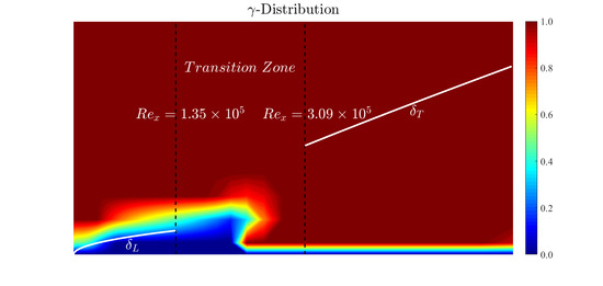
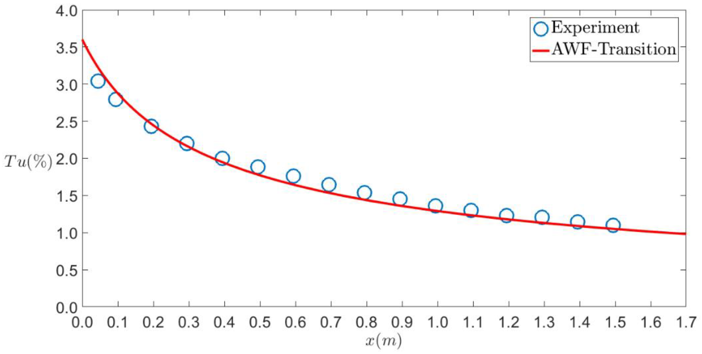
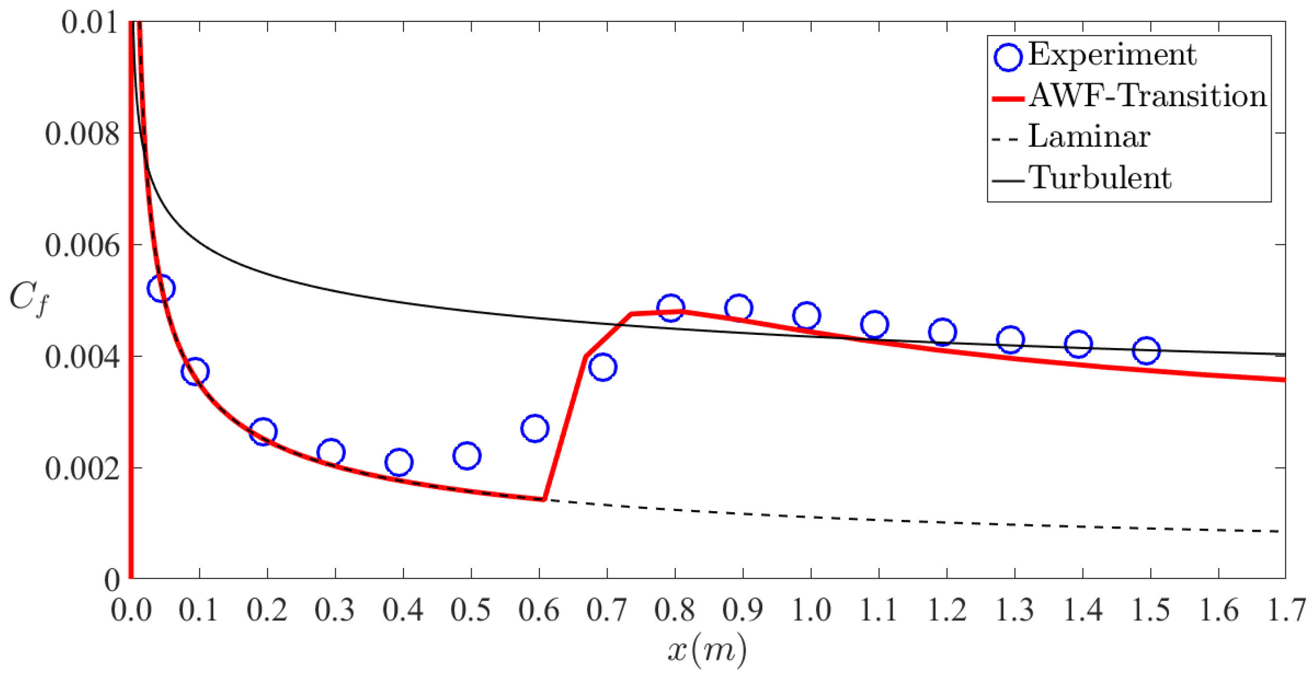
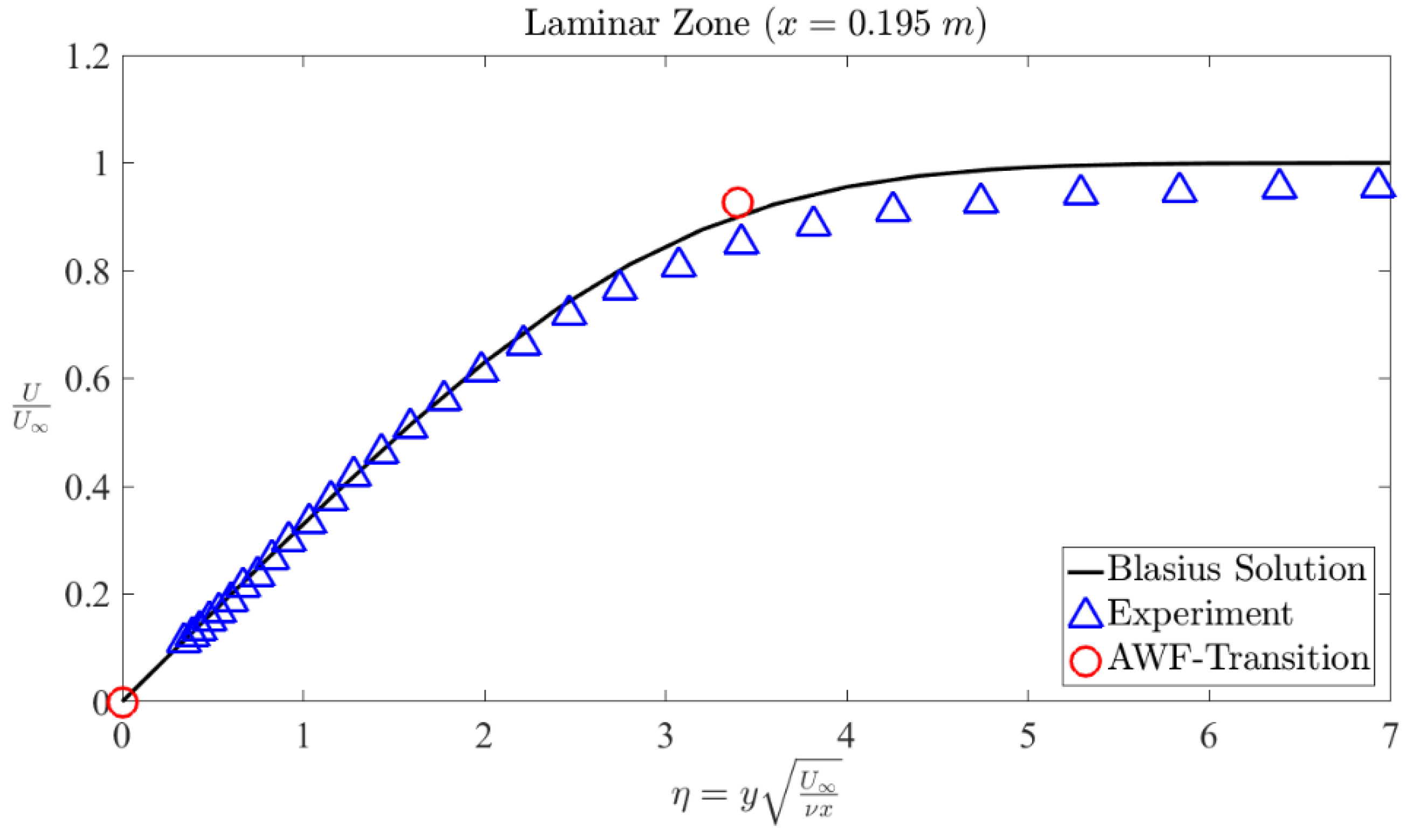
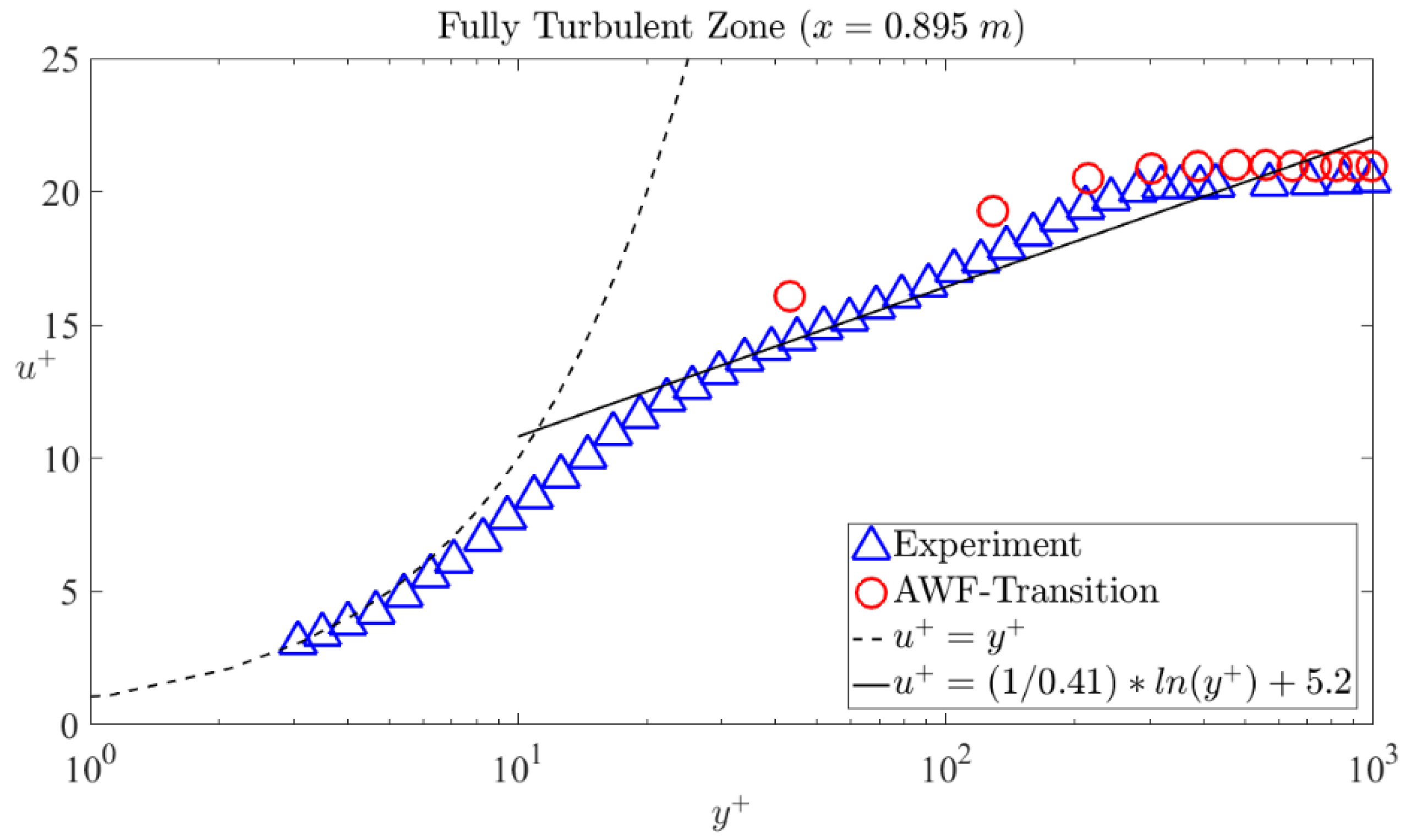
4. Results and Discussion

The present AWF in combination with the currently modified versions of the k ω turbulence model of Wilcox [46] and the algebraic γ transition model of Kubacki and Dick [43,44], hereafter AWF-transition, is implemented into an in-house CFD code which is based on the cell-centered finite-volume method. The convection terms are discretized by the QUICK scheme while the second-order central difference scheme is used for the diffusion terms. The SIMPLE algorithm is employed to couple the pressure and the velocity. The Rhie–Chow interpolation is used to handle the collocated grid arrangement. The convergence criteria is set to be equal to 10−4.
The standard T3A test case of ERCOFTAC by Coupland [48] is used to validate the proposed AWF-transition formulation for predicting bypass transition. The computational domain and boundary conditions of T3A are illustrated in Figure 1. The structured mesh used is composed of 300 (clustering near the leading edge) × 100 (uniform with Δ y + 40 at outlet) in the x- and y-directions, respectively, which is selected after performing grid-independent study. The mesh distribution is displayed in Figure 2. The flow condition of T3A is summarized in Table 1.
Using the inlet condition in Table 1, the decay of the free-stream turbulence intensity is well matched between the prediction and the experimental data in the case of T3A, as shown in Figure 3.
Figure 4 shows the skin friction coefficient distribution along a flat plate where the AWF-transition result is compared with the experimental data. It reveals that the present AWF-transition can capture the laminar-to-turbulent flow transition, although a coarse mesh is employed.
The mean velocity profile at x = 0.695   m in the transition zone is plotted in wall units ( u + = U / u τ , y + = y u τ / ν ) and in the same dimensionless form as Blasius solution ( U / U , η = y U / ν x ) in Figure 5a,b, respectively, where the AWF-transition result is compared with the experimental data in both scaling forms, including the law of the wall in Figure 5a and the Blasius solution in Figure 5b. It reveals that the present AWF-transition is capable of predicting the mean velocity profile in the transition zone. It can be noticed from the experimental data that the flow is neither fully turbulent nor laminar because the log layer is not yet established and the Blasius solution is no longer valid at this location in the transition zone.
In Figure 6, the velocity profile at x = 0.195   m in the laminar zone is shown where the AWF-transition result is compared with both the experimental data and the Blasius solution. Even though there are very few grid points in the wall-normal direction inside the laminar boundary layer, the AWF-transition result agrees well with both the experimental data and the Blasius solution.
In Figure 7, the mean velocity profile at x = 0.895   m in the fully turbulent zone is plotted in wall units, where the AWF-transition result is compared with both the experimental data and the law of the wall. The AWF-transition result is in good agreement with the experimental data and the law of the wall. At this location in the fully turbulent zone, the log layer is well established as demonstrated by the experimental data and also the AWF-transition result. However, the AWF-transition result is slightly over-predicted compared to the experimental data.

5. Conclusions

In this work, the capability of AWF was extended to the prediction of the bypass-transition effect on the mean flow. To capture the transition onset and the transition process, the presently modified versions of the algebraic γ transition model of Kubacki and Dick [43,44] and the k ω turbulence model of Wilcox [46] were integrated into the proposed AWF-transition of an in-house CFD code. For validation, the T3A test case of bypass transition was used. This AWF-transition showed the predictive capability of detecting the transition onset and the transition process in the distribution of C f over a flat plate. Moreover, the mean velocity profiles were well predicted in laminar, transitional and fully turbulent regions.

Author Contributions

Conceptualization, E.J., K.N., K.S.; methodology, E.J., K.N.; software, K.N.; validation, K.N.; formal analysis, E.J., K.N.; investigation, E.J., K.N., K.S.; resources, E.J., K.S.; data curation, K.N., P.T.; writing—original draft preparation, E.J.; writing—review and editing, E.J., K.N., P.T.; visualization, K.N.; supervision, K.S.; project administration, E.J.; funding acquisition, E.J. All authors have read and agreed to the published version of the manuscript.

Funding

This research was funded by King Mongkut’s University of Technology North Bangkok [Contract no. KMUTNB-61-GOV-B-36].

Institutional Review Board Statement

Not applicable.

Acknowledgments

Authors would like to thank King Mongkut’s University of Technology North Bangkok.

Conflicts of Interest

The authors declare no conflict of interest.

References

  1. Balonishnikov, A.M. Simplified description of small-scale turbulence. Tech. Phys. 2003, 48, 1407–1412. [Google Scholar] [CrossRef]
  2. Ershkov, S. About existence of stationary points for the Arnold–Beltrami–Childress (ABC) flow. Appl. Math. Comput. 2016, 276, 379–383. [Google Scholar] [CrossRef] [Green Version]
  3. Pacciani, R.; Marconcini, M.; Fadai-Ghotbi, A.; Lardeau, S.; Leschziner, M.A. Calculation of high-lift cascades in low pressure turbine conditions using a three-equation model. J. Turbomach. 2011, 133, 031016. [Google Scholar] [CrossRef]
  4. Pacciani, R.; Marconcini, M.; Arnone, A.; Bertini, F. Predicting high-lift low-pressure turbine cascades flow using transition-sensitive turbulence closures. J. Turbomach. 2013, 136, 051007. [Google Scholar] [CrossRef]
  5. Patankar, S.V.; Spalding, D.B. Heat and Mass Transfer in Boundary Layers; Morgan-Grampian Press: London, UK, 1967. [Google Scholar]
  6. Launder, B.E.; Spalding, D.B. The numerical computation of turbulent flows. Comput. Methods Appl. Mech. Eng. 1974, 3, 269–289. [Google Scholar] [CrossRef]
  7. Hanjalić, K.; Launder, B. Modelling Turbulence in Engineering and the Environment: Second-Moment Routes to Closure; Cambridge University Press: Cambridge, UK, 2011. [Google Scholar]
  8. Saric, S.; Basara, B.; Suga, K.; Gomboc, S. Analytical wall-function strategy for the modelling of turbulent heat transfer in the automotive CFD applications. SAE Tech. Paper 2019. [Google Scholar] [CrossRef]
  9. Craft, T.J.; Gerasimov, A.V.; Iacovides, H.; Launder, B.E. Progress in the generalization of wall-function treatments. Int. J. Heat Fluid Flow 2002, 23, 148–160. [Google Scholar] [CrossRef]
  10. Craft, T.J.; Gerasimov, A.V.; Iacovides, H.; Kidger, J.W.; Launder, B.E. The negatively buoyant turbulent wall jet: Performance of alternative options in RANS modelling. Int. J. Heat Fluid Flow 2004, 25, 809–823. [Google Scholar] [CrossRef]
  11. Suga, K.; Craft, T.J.; Iacovides, H. An analytical wall-function for turbulent flows and heat transfer over rough walls. Int. J. Heat Fluid Flow 2006, 27, 852–866. [Google Scholar] [CrossRef]
  12. Suga, K. Computation of high Prandtl number turbulent thermal fields by the analytical wall-function. Int. J. Heat Mass Transf. 2007, 50, 4967–4974. [Google Scholar] [CrossRef]
  13. Suga, K.; Nishiguchi, S. Computation of turbulent flows over porous/fluid interfaces. Fluid Dyn. Res. 2009, 41, 012401. [Google Scholar] [CrossRef]
  14. Suga, K.; Kubo, M. Modelling turbulent high Schmidt number mass transfer across undeformable gas–liquid interfaces. Int. J. Heat Mass Transf. 2010, 53, 2989–2995. [Google Scholar] [CrossRef]
  15. Suga, K.; Ishibashi, Y.; Kuwata, Y. An analytical wall-function for recirculating and impinging turbulent heat transfer. Int. J. Heat Fluid Flow 2013, 41, 45–54. [Google Scholar] [CrossRef]
  16. Amano, R.S.; Arakawa, H.; Suga, K. Turbulent heat transfer in a two-pass cooling channel by several wall turbulence models. Int. J. Heat Mass Transf. 2014, 77, 406–418. [Google Scholar] [CrossRef]
  17. Omranian, A.; Craft, T.J.; Iacovides, H. The computation of buoyant flows in differentially heated inclined cavities. Int. J. Heat Mass Transf. 2014, 77, 1–16. [Google Scholar] [CrossRef]
  18. Wang, X.; Craft, T.J.; Iacovides, H. An analytical wall function for 2-D shock wave/turbulent boundary layer interactions. In Proceedings of the 3rd World Congress on Mechanical, Chemical, and Material Engineering (MCM’17), Rome, Italy, 9–10 June 2017; pp. 7–10. [Google Scholar] [CrossRef]
  19. Chedevergne, F. Analytical wall function including roughness corrections. Int. J. Heat Fluid Flow 2018, 73, 258–269. [Google Scholar] [CrossRef] [Green Version]
  20. Aupoix, B. Improved heat transfer predictions on rough surfaces. Int. J. Heat Fluid Flow 2015, 56, 160–171. [Google Scholar] [CrossRef]
  21. Aupoix, B. Roughness corrections for the k–ω shear stress transport model: Status and proposals. J. Fluids Eng. 2015, 137, 021202. [Google Scholar] [CrossRef]
  22. Suga, K. Amendments to the extended analytical wall function for turbulent high Prandtl number flows. In Turbulence, Heat and Mass Transfer; Hanjalić, K., Nagano, Y., Jakirlić, S., Eds.; Begell House Inc.: Danbury, CT, USA, 2006; Volume 5. [Google Scholar]
  23. Fu, S.; Wang, L. RANS modeling of high-speed aerodynamic flow transition with consideration of stability theory. Prog. Aerosp. Sci. 2013, 58, 36–59. [Google Scholar] [CrossRef]
  24. Durbin, P.A. Perspectives on the phenomenology and modeling of boundary layer transition. Flow Turbul. Combust. 2017, 99, 1–23. [Google Scholar] [CrossRef]
  25. Durbin, P.A. Some recent developments in turbulence closure modeling. Annu. Rev. Fluid Mech. 2018, 50, 77–103. [Google Scholar] [CrossRef]
  26. Dick, E.; Kubacki, S. Transition models for turbomachinery boundary layer flows: A review. Int. J. Turbomach. Propuls. Power 2017, 2, 4. [Google Scholar] [CrossRef] [Green Version]
  27. Langtry, R.B.; Menter, F.R. Correlation-based transition modeling for unstructured parallelized computational fluid dynamics codes. AIAA J. 2009, 47, 2894–2906. [Google Scholar] [CrossRef]
  28. Juntasaro, E.; Ngiamsoongnirn, K. A new physics-based γ-kL transition model. Int. J. Comput. Fluid Dyn. 2014, 28, 204–218. [Google Scholar] [CrossRef]
  29. Juntasaro, E.; Narejo, A.A. A γ-kL Transition model for transitional flow with pressure gradient effects. Eng. J. 2017, 21, 279–304. [Google Scholar] [CrossRef]
  30. Xu, J.K.; Bai, J.Q.; Qiao, L.; Zhang, Y.; Fu, Z.Y. Fully local formulation of a transition closure model for transitional flow simulations. AIAA J. 2016, 54, 3015–3023. [Google Scholar] [CrossRef]
  31. Xu, J.K.; Bai, J.Q.; Fu, Z.Y.; Qiao, L.; Zhang, Y.; Xu, J.L. Parallel compatible transition closure model for high-speed transitional Flow. AIAA J. 2017, 55, 3040–3050. [Google Scholar] [CrossRef]
  32. Lodefier, K.; Merci, B.; De Langhe, C.; Dick, E. Transition modelling with the k-Ω turbulence model and an intermittency transport equation. J. Therm. Sci. 2004, 13, 220–225. [Google Scholar] [CrossRef]
  33. Wang, L.; Fu, S. Development of an intermittency equation for the modeling of the supersonic/hypersonic boundary layer flow transition. Flow, Turbul. Combust. 2011, 87, 165–187. [Google Scholar] [CrossRef]
  34. Durbin, P.A. An intermittency model for bypass transition. Int. J. Heat Fluid Flow 2012, 36, 1–6. [Google Scholar] [CrossRef]
  35. Ge, X.; Arolla, S.; Durbin, P. A Bypass transition model based on the intermittency function. Flow Turbul. Combust. 2014, 93, 37–61. [Google Scholar] [CrossRef]
  36. Menter, F.R.; Smirnov, P.E.; Liu, T.; Avancha, R. A one-equation local correlation-based transition model. Flow Turbul. Combust. 2015, 95, 583–619. [Google Scholar] [CrossRef]
  37. Juntasaro, E.; Ngiamsoongnirn, K.; Thawornsathit, P.; Durbin, P. Development of an intermittency transport equation for modeling bypass, natural and separation-induced transition. J. Turbul. 2021, 22, 562–595. [Google Scholar] [CrossRef]
  38. Mayle, R.E.; Schulz, A. Heat transfer committee and turbomachinery committee best paper of 1996 award: The path to predicting bypass transition. J. Turbomach. 1997, 119, 405–411. [Google Scholar] [CrossRef]
  39. Walters, D.K.; Leylek, J.H. A new model for boundary layer transition using a single-point RANS approach. J. Turbomach. 2004, 126, 193–202. [Google Scholar] [CrossRef]
  40. Walters, D.K.; Cokljat, D. A three-equation eddy-viscosity model for Reynolds-Averaged Navier–Stokes simulations of transitional flow. J. Fluids Eng. 2008, 130, 121401. [Google Scholar] [CrossRef]
  41. Medina, H.; Beechook, A.; Fadhila, H.; Aleksandrova, S.; Benjamin, S. A novel laminar kinetic energy model for the prediction of pretransitional velocity fluctuations and boundary layer transition. Int. J. Heat Fluid Flow 2018, 69, 150–163. [Google Scholar] [CrossRef]
  42. Lopez, M.; Walters, D.K. Prediction of transitional and fully turbulent flow using an alternative to the laminar kinetic energy approach. J. Turbul. 2016, 17, 253–273. [Google Scholar] [CrossRef]
  43. Kubacki, S.; Dick, E. An algebraic model for bypass transition in turbomachinery boundary layer flows. Int. J. Heat Fluid Flow 2016, 58, 68–83. [Google Scholar] [CrossRef]
  44. Kubacki, S.; Dick, E. An algebraic intermittency model for bypass, separation-induced and wake-induced transition. Int. J. Heat Fluid Flow 2016, 62, 344–361. [Google Scholar] [CrossRef]
  45. Sandhu, J.P.S.; Ghosh, S. A local correlation-based zero-equation transition model. Comput Fluids 2021, 214, 104758. [Google Scholar] [CrossRef]
  46. Wilcox, D.C. Formulation of the k-ω turbulence model revisited. AIAA J. 2008, 46, 2823–2838. [Google Scholar] [CrossRef] [Green Version]
  47. Suga, K. Analytical wall-functions of turbulence for complex surface flow phenomena. Comput. Fluid Dyn. Heat Transf. Emerg. Top. 2010, 41, 331–380. [Google Scholar] [CrossRef]
  48. ERCOFTAC Classic Collection Database. Coupland (1990). Available online: http://cfd.mace.manchester.ac.uk/ercoftac (accessed on 1 May 2005).
Figure 1. Computational domain and boundary conditions of T3A.
Fluids 06 00328 g001
Figure 2. Mesh distribution displayed at every fifth line.
Fluids 06 00328 g002
Figure 3. Decay of free-stream turbulence intensity of T3A.
Fluids 06 00328 g003
Figure 4. Skin friction coefficient distribution along a flat plate of T3A.
Fluids 06 00328 g004
Figure 5. Mean velocity profile of T3A in the transition zone: (a) plotted in wall units and (b) plotted in the same dimensionless form as Blasius solution.
Fluids 06 00328 g005
Figure 6. Velocity profile of T3A in the laminar zone.
Fluids 06 00328 g006
Figure 7. Mean velocity profile of T3A plotted in wall units in the fully turbulent zone.
Fluids 06 00328 g007
Table 1. Flow condition of T3A.
Test Case U   ( m / s ) T u   ( % ) Viscosity Ratio ( ν T / ν ) R e L
T3A5.43.6126.1 × 105
Publisher’s Note: MDPI stays neutral with regard to jurisdictional claims in published maps and institutional affiliations.

