A Deep Learning Approach for Wave Forecasting Based on a Spatially Correlated Wind Feature, with a Case Study in the Java Sea, Indonesia

Abstract

For safety and survival at sea and on the shore, wave predictions are essential for marine-related activities, such as harbor operations, naval navigation, and other coastal and offshore activities. In general, wave height predictions rely heavily on numerical simulations. The computational cost of such a simulation can be very high (and it can be time-consuming), especially when considering a complex coastal area, since these simulations require high-resolution grids. This study utilized a deep learning technique called bidirectional long short-term memory (BiLSTM) for wave forecasting to save computing time and to produce accurate predictions. The deep learning method was trained using wave data obtained by a continuous numerical wave simulation using the SWAN wave model over a 20-year period with ECMWF ERA-5 wind data. We utilized highly spatially correlated wind as input for the deep learning method to select the best feature for wave forecasting. We chose an area with a complex geometry as the study case, an area in Indonesia’s Java Sea. We also compared the results of wave prediction using BiLSTM with those of other methods, i.e., LSTM, support vector regression (SVR), and a generalized regression neural network (GRNN). The forecasting results using the BiLSTM were the best, with a correlation coefficient of 0.96 and an RMSE value of 0.06.

1. Introduction

Shipping and other marine-related operations are highly dependent on weather conditions. A range of technologies, methodologies, and historical data are used to forecast future weather conditions [1]. The height of the sea waves is a critical meteorological condition. The length of a wave height forecast is often determined by the significance of the activity [2]. High sea waves might endanger a ship by overturning it, resulting in significant losses. This can be prevented by optimizing the shipping route. Consequently, forecasting wave height might help to avoid dangerous conditions while simultaneously enhancing productivity and preserving fuel [3]. Moreover, as carbon dioxide levels increase, one of the mitigation strategies is to use renewable energy resources efficiently [4]. Waves at sea can be considered one renewable energy source, since they continuously propagate as the wind blows. Therefore, it is critical to estimate wave heights accurately to provide an overview of current ocean wave conditions [5].

Predicting the height of a sea wave is challenging due to their stochastic nature and nonlinear characteristics [6]. Consequently, research on wave height prediction is continuously being updated to keep increasing the accuracy of predictions and the computational speed of wave forecasting systems [7]. In classic numerical approaches, wave height prediction is accomplished by three factors: the physical formulation, numerical discretization, and simulation [8], all of which are dependent on the input data provided. The three most preferred phase-averaged wave models simulate wave generation and propagation, and they are usually called the so-called third-generation wave models: WAM [9], SWAN [10], and WAVEWATCH III [11]. All are examples of numerical simulations in the spatial domain. The WAM and WAVEWATCH III models are intended for simulating large-domain or ocean-scale waves, since their direct temporal integration is incompatible with complicated shoreline scales [12]. In comparison, the SWAN model is often used to forecast ocean waves at a local scale using regional forecasts [13]. Indeed, since they are based on numerical simulations, they also come with some consequences: to calculate wave propagation in environments with complex geometries, high-resolution grids are needed, and they require powerful computational resources and a long period of time [14].

An alternative approach to numerical simulations is the soft computing approach, which can calculate faster predictions than the numerical approaches while maintaining lower computational costs. The soft computing approach is not new in wave prediction, particularly with respect to neural networks. Several studies have used different approaches to forecast wave height. Alexandre et al. established forecasts with a Root Mean Square Error (RMSE) of 0.75 and an RMSE of 0.5 in two scenarios in the Western Atlantic and the Caribbean Sea, respectively [15]. In 2017, Nikoo et al. demonstrated that fuzzy KNN and regression tree induction models outperform other soft computing models [16]. Zubier used an artificial neural network (ANN), specifically NARX, to forecast waves on the Red Sea in 2018, with excellent results for 3–24 h forecasts [17]. The MSE was only 0.07. Wang et al. discovered that using residual learning to adjust a numerical model was more accurate and efficient than using a numerical technique [18] for predictions within 3–72 h. In 2019, Elbisy employed the group method of a data-handling-type neural network (GMDH-NN) and the multilayer perceptron neural network (MLPNN) to estimate wave heights [19]. They concluded that the GMDH-NN produces better predictions than the MLPNN. Tong Liu et al. used a deep learning algorithm called WaveNet that can produce wave patterns more similar to buoy measurements than numerical simulations [20]. In 2020, Callens et al. employed a random forest and gradient boosting to enhance the prediction accuracy at particular sites [21]. Chen et al. used the wavelet graph neural network to predict wave height and compared it to other ANN models, finding that it outperformed other models by 16.4% [3]. Ting Yu used the convolutional gated recurrent unit network to provide one-hour predictions with a correlation coefficient of 0.996 and an RMSE of 0.136 [22]. The above-mentioned wave forecasting methods are generally used to forecast waves 3–72 h ahead. For coastal and offshore operational activities, especially for the scheduling of ship transportation, a longer forecasting time interval is needed, i.e., 7–14 days ahead. The wave height mentioned here is the significant wave height.

The forecasting method affects the accuracy of the wave prediction, but the geometry of the study area may also significantly affect the accuracy of the prediction. For a numerical approach, forecasting waves in a geometrically complex area, such as a coastal area, requires wave simulation with a high-resolution grid, which will lead to time-consuming computation. For a machine-learning-based wave forecasting model, the accuracy of the data for the machine learning training process significantly affects the forecasting system’s accuracy. Herein, we walk through the design of an efficient wave forecasting system built for rapid wave height predictions with acceptable accuracy. We propose a novel approach to designing a complex coastal area wave forecasting system. 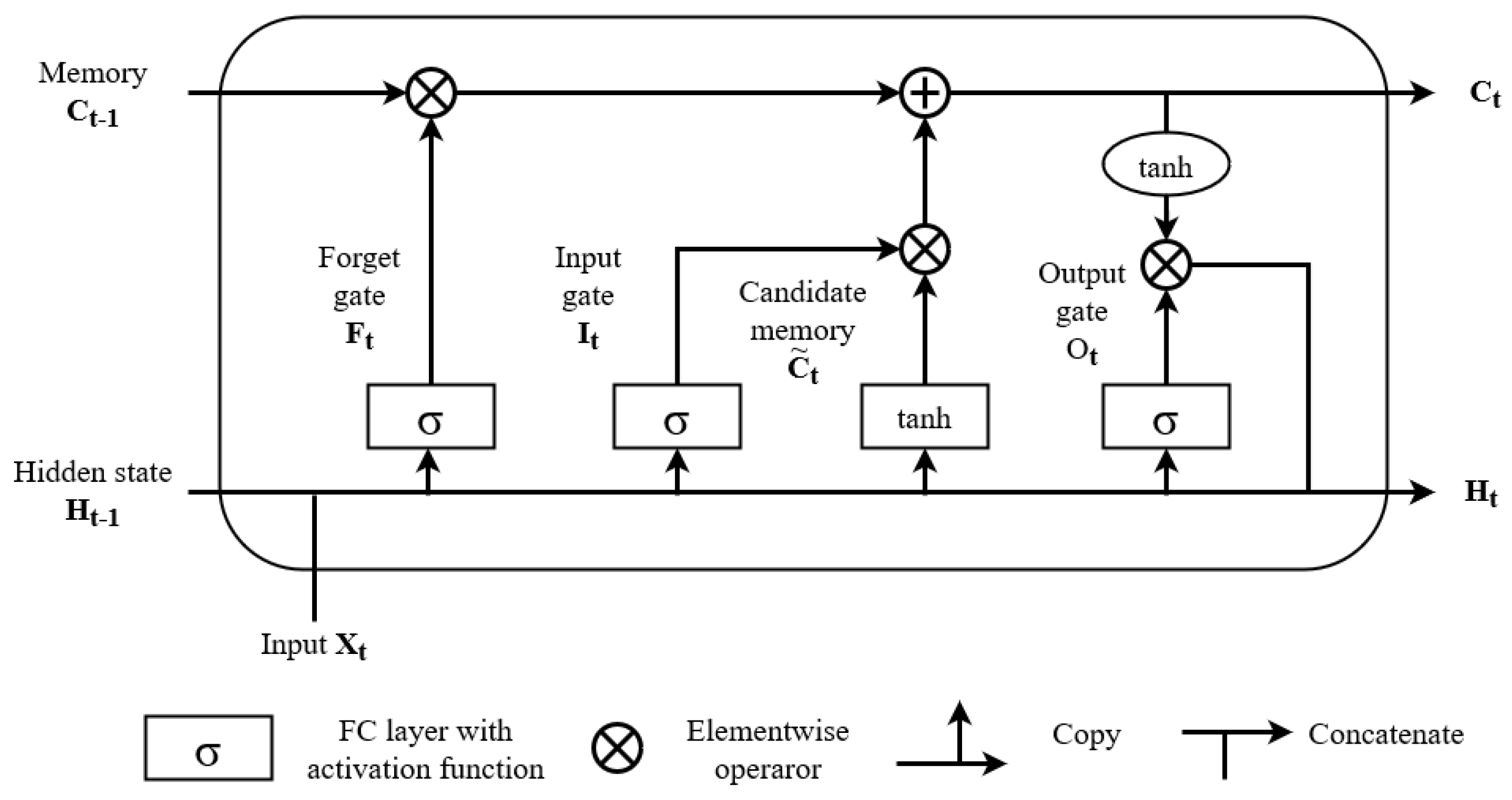We combine high-resolution wave simulations using the SWAN wave model [10] with a deep learning method called bidirectional long short-term memory (BiLSTM) to process wind information to predict significant wave height. We used the SWAN model to generate high-resolution training data in a coastal area with a complex geometry. For validation, we compared the numerical simulation results generated with the SWAN model, with available observation wave data from the Java Sea, Indonesia. The deep learning BiLSTM method was trained using wave data obtained from a continuous numerical wave simulation using the SWAN model over a 20 year-period with ECMWF ERA-5 wind data [23]. We used highly spatially correlated wind as input for the deep learning method to select the best feature for significant wave forecasting. We chose an area with a complex geometry as the study case, an area in Indonesia’s Java Sea. Moreover, we also compared the results of wave prediction using BiLSTM with the results of other methods, i.e., LSTM, support vector regression (SVR), and a generalized regression neural network (GRNN).

The study area in the Java Sea was chosen since it is considered to have a complex geometry, in a relatively shallow coastal area. There have been several studies conducted in this study area. For example, in 2015, Rizkina et al. predicted the height of sea waves in the Java Sea using a simple ANN, which produced reasonably accurate prediction results with an RMSE of 0.06 m. In predicting it themselves, they used three inputs in the model, namely wave height, wind speed, and wind direction, to obtain the next wave height [15]. In 2017, Dhanista et al. employed a neural network to forecast significant wave height in the Java Sea, especially in Northern Surabaya, and obtained favorable results for predicting 1 h and 6 h, with RMSE values of 0.03 and 0.09, respectively [24]. In 2020, Vita Juliani et al. employed a GRNN to forecast the Jakarta Bay region, achieving a correlation coefficient of 0.92 and an RMSE of 0.13 [25]. This paper aims to provide a better deep-learning-based significant wave forecasting method with the wind as the main feature of the deep learning input.

This paper is organized as follows: Section 2 describes a brief description of the wave model and deep learning methods used in this study. Section 3 describes the methodology to design the wave forecasting system, including data generation, exploratory data, and machine learning optimization. Results and discussions are presented in Section 5. We conclude the paper in the last section.

2. Literature Review

We aimed to design a wave forecasting system based on combined high-resolution wave simulation using the SWAN model with the deep learning method BiLSTM. The SWAN simulation aims to generate high-resolution wave simulation for training data, whereas we used ECMWF-ERA5 wind data as the primary input for the wave simulation. The deep learning method was used to solve the supervised learning problem, i.e., a regression problem that calculates wave height from wind field. In this section, we briefly discuss the basic idea of the SWAN model and the BiLSTM model.

2.1. SWAN Model (Simulated Waves Nearshore)

The SWAN or Simulating Waves Nearshore is a third-generation spectral wave model that was first introduced by Booij et al. [10]. The SWAN model is designed for wave generation and propagation, especially in small-scale coastal sites with shallow water, local winds, (barrier) islands, and tidal flats [26]. Physical processes such as wave generation, white capping, quadruplet wave–wave interactions, and bottom dissipation processes are all modeled in the same way as in previous third-generation wave models [10]. The SWAN calculated the wave energy as they propagated across the ocean and fanned out along the shore [27]. This paper uses the most recent version of the SWAN model, i.e., version 41.20. The governing equation in the SWAN model is based on the spectral action balancing equation that is given as follows:

$$\frac{S(\sigma ,\theta ;x,y,t)}{\sigma }=\frac{\partial N}{\partial t}+\left(\frac{\partial C_{x}N}{\partial x}+\frac{\partial C_{y}N}{\partial y}\right)+\frac{\partial C_{\sigma }N}{\partial \sigma }+\frac{\partial C_{\theta }N}{\partial \sigma }$$

(1)

where the entire source term is denoted by the $S(\sigma ,\theta ;x,y,t)$ term. The action balance equation’s source terms represent the effects of generation, dissipation, and nonlinear wave–wave interactions. N is the action density expressed as an intrinsic frequency function of the horizontal coordinates x and y, the relative frequency $\sigma$, the wave direction $\theta$, and the time constant t. $C_{\sigma }$ and $C_{\theta }$ are the propagation speeds in spectral space ($sigma$ and $theta$, respectively), whereas $C_x$ and $C_y$ are components of the velocity group x and y, respectively. Three processes contributed to the sink and source terms S in the SWAN model are defined as follows:

$$S=S_{in}+S_{ds}+S_{nl}$$

(2)

where $S_{in}$ denotes the development of waves induced by the wind. Dissipation generated by bottom friction, white capping, and depth-induced wave breaking is represented by the symbol $S_{ds}$. Finally, the final $S_{nl}$ may be thought of as a nonlinear transfer of wave energy caused by wave–wave interactions. The SWAN model was used in this study to simulate wind data from ECMWF-ERA-5 in the domain of Java Sea, Indonesia, to generate training data from the deep learning method BiLSTM. In the following subsection, we describe the idea of Long Short-Term Memory (LSTM) and BiLSTM.

2.2. Long Short-Term Memory

Long Short-Term Memory, or LSTM, is an advanced variant of a deep learning model for sequential data called the Recurrent Neural Network (RNN) [28]. The RNN was developed in the 1980s [29]. Since the RNN has a limitation in memory for understanding long-term dependencies, an LSTM-based model is used to address this limitation. Sepp Hochreiter and Jürgen Schmidhuber Schmidhuber invented LSTM in 1997 [28]. Essentially, the LSTM model may augment the RNN’s memory, enabling it to store and learn long-term input dependencies.

The architecture of LSTM introduces the so-called memory cell that is used to store information. As shown in Figure 1, three gates control the memory cell: the input gate, forget gate, and output gate. The input gate is used to read data, the forget gate is used to memorize some of the data and throw away the rest of the data, and the output gate is used to read out the entries from the cell [30]. To describe the architecture, we introduce some notations: $X_t$ and $H_t$ denote the input state and the hidden state at time step t. In the LSTM architecture, the data are fed into the memory cell from $X_t$ and $H_{(t-1)}$ and then is processed into three gates, namely the forget gate, the input gate, and the output gate. These three gates are normalized using the sigmoid activation function, denoted as $\sigma$, such that this information has a value between 0 and 1. This information is calculated using the following formula:

$$\begin{array}{c}\hfill F_t=\sigma (X_t{W}_{xf}+H_{t-1}Whf+b_f)\\ \hfill I_t=\sigma (X_t{W}_{xi}+H_{t-1}Whi+b_i)\\ \hfill O_t=\sigma (X_t{W}_{xo}+H_{t-1}Who+b_o)\end{array}$$

(3)

where $W_{xf}$, $W_{xi}$, and $W_{xo}$ denote the input $X_t$ weights corresponding to the forget, input, and output gates, respectively. The notations $W_{hf}$, $W_{hi}$, and $W_{ho}$ are also similar, denoting the hidden state $H_{(t-1)}$ weights corresponding to the forget, input, and output gates, respectively. $b_f$, $b_i$, and $b_o$ denote bias parameters corresponding to the forget, input, and output gates, respectively. Other than these three gates, i.e., the input, forget, and output gates, the LSTM architecture also introduces a gate for a candidate for memory cell called candidate gate ${\tilde{C}}_t$, which is calculated using the following formula:

$${\tilde{C}}_t=tanh(X_t{W}_{xc}+H_{t-1}Whc+b_c).$$

(4)

In contrast to the other gates, in the candidate gate, the information is normalized using the activation function tanh, such that the value of ${\tilde{C}}_t$ is between −1 to 1. The notations $W_{xc}$, $W_{hc}$, and $b_c$ denote weight values for the input state, the hidden state, and the bias, respectively. Using values from candidate gate ${\tilde{C}}_t$, forget gate $F_t$, and input date $I_t$, the memory cell content $C_t$ is updated using the following formula:

$$C_t=F_t\times C_{t-1}+I_t\times {\tilde{C}}_t$$

(5)

where × denotes element-wise multiplication. Note that the forget gate $F_t$ has a value between 0 and 1 since it is normalized using the sigmoid activation function. This means that if the value is 0, then no memory is passed, whereas if $F_t$ is 1, all memory will be passed into the next state.

2.3. Bidirectional Long Short-Term Memory

The BiLSTM model is a combination between the Bidirectional RNN (BiRNN) and LSTM. Schuster and Paliwal presented the BiRNN for the first time in 1997 [31]. In the BiRNN, two RNN architectures, namely the forward and backward RNNs, are combined. In the BiLSTM model, the architecture of the RNN is replaced with LSTM architecture to overcome the vanishing and exploding gradient problem in the RNN [32]. Graves and Schmidhuber [33] then presented the BiLSTM technique in 2005, a modified and full gradient version of the LSTM.

The architecture of the BiLSTM is illustrated in Figure 2. To describe the architecture of the BiLSTM, we introduce some notations, ${\overrightarrow{H}}_t$ and ${\overleftarrow{H}}_t$, for the forward and backward hidden states. These hidden states are calculated using the following formula:

$$\begin{array}{c}\hfill {\overrightarrow{H}}_t=A(X_t{W}_{xh}^{Forw}+{\overrightarrow{H}}_{t-1}{W}_{hh}^{Forw}+b_h^{Forw})\\ \hfill {\overleftarrow{H}}_t=A(X_t{W}_{xh}^{Back}+{\overleftarrow{H}}_{t-1}{W}_{hh}^{Back}+b_h^{Back}).\end{array}$$

(6)

where $W_{xh}^{Forw}$ and $W_{xh}^{Back}$ denote the weight values for forward and backward input $X_t$, respectively, whereas $W_{hh}^{Forw}$ and $W_{hh}^{Back}$ denote the weight values for the forward and backward hidden state ${\overrightarrow{H}}_{t-1}$ and ${\overleftarrow{H}}_{t-1}$. $b_h^{Forw}$ and $b_h^{Back}$ denote the bias value for the forward and backward state. A denotes the activation function for the hidden layer. From these values of ${\overrightarrow{H}}_t$ and ${\overleftarrow{H}}_t$, the hidden state $H_t$ can be obtained by concatenating ${\overrightarrow{H}}_t$ and ${\overleftarrow{H}}_t$. Lastly, the output state can be calculated using $H_t$ with the following formula:

$$O_t=H_t{W}_o+b_o$$

(7)

where $W_o$ and $b_o$ are the weight and bias value in the output layer [30].

3. Methodology

We designed a wave forecasting system based on a combined high-resolution numerical simulation with a deep learning model; there were three main steps in designing the system. The initial step was to build a wave dataset from wind field data by performing continuous-wave simulation using the SWAN model. In the second step, the obtained wave dataset and wind field data from the previous step were used for exploratory data to investigate the best feature to be used as input for the deep learning BiLSTM method. Here, we calculated the spatial correlation between wind field data and wave height at the study area, i.e., in Jakarta Bay, Java Sea, Indonesia. The last step was to optimize the deep learning algorithm to obtain the best forecasting accuracy. Moreover, we also compared the results of wave forecasting using BiLSTM with other machine learning models, such as LSTM, Support Vector Regression (SVR), and the Generalized Regression Neural Network (GRNN).

3.1. Wave Data Generation

For predicting waves in environments with a complex geometry, such as in a coastal area with many small islands, high-resolution wave simulation is needed, especially to better represent the simulation domain’s geometry. We used the SWAN model to generate high-resolution training data by performing continuous-wave simulation with the ECMWF ERA-5 wind data. The simulation procedure for obtaining significant wave height data is depicted in Figure 3. The initial step was to prepare wind and bathymetry data for the wave simulation. As mentioned previously, we used hourly ECMWF ERA-5 wind data [23] for the last 20 years (2000–2020). We used the bathymetry provided by GEBCO (General Bathymetric Chart of the Oceans) for simulation in the global domain, whereas we used Indonesia’s BATNAS (National Bathymetry) for the location domain.

The wave data here consists of the significant wave height (Hs), peak wave period (Tp), and mean wave direction. To obtain accurate wave data for an environment with a complex geometry and a rather shallow bathymetry, such as in the Java Sea, we performed nested simulations consisting of 2 nested domains. These nested simulations were aimed to obtain a high-resolution simulation in our study area, in Jakarta Bay, Java Sea, Indonesia. Firstly, we simulated wave conditions in a global domain as shown in Figure 4. Secondly, we simulated wave conditions and, in addition, obtained boundary conditions from the global simulation to simulate wave propagation in an intermediate domain, as shown in Figure 5. Lastly, we simulated the wave propagation in a local domain in Jakarta Bay, Java Sea, by using boundary conditions obtained from the intermediate domain, as shown in Figure 6. Figure 4, Figure 5 and Figure 6 show snapshots of the wind field (left part) and the resulting significant wave height (right part) on 6 December 2020 at 06:00 UTC.

The numerical setting for these three domains is shown in

Table 1. Numerical configuration for nested wave simulation.

Domain	Longitude(${}^{\circ }$)		Latitude(${}^{\circ }$)		$\Delta \mathit{x}$	$\Delta \mathit{y}$	Nx	Ny
	From	To	From	To
1	0.50	175.50	−69.50	30.50	1.5000	1.5000	117	67
2	100.00	132.00	−15.00	5.00	0.2500	0.2500	128	80
3	106.65	107.05	−6.12	−5.86	0.00267	0.00267	150	99

. Here, $\Delta x$ and $\Delta y$ denote the spatial grid size in longitude and latitude. $Nx$ and $Ny$ represent the number of discretization points in longitude and latitude. For the global and intermediate domains, we used spatial grid sizes of $1.5^{\circ }$ and $0.{25}^{\circ }$, respectively, whereas to accurately represent the geometry of the local domain in Jakarta Bay, we used a spatial resolution of 0.00267${}^{\circ }$.

To test the accuracy of the resulting wave simulation, we compared the results of SWAN simulation with available wave observations in Jakarta Bay, Java Sea, Indonesia. The data on wave observations of the location 106.7654${}^{\circ }$ E and 6.0108${}^{\circ }$ S in Jakarta Bay, Java Sea, from 21 January–2 February 2017 are shown in Figure 7. Results of the SWAN simulation, compared with observation data, waves from ERA-5, and waves from The Global Forecast System (GFS) from the National Oceanic and Atmospheric Administration (NOAA), are shown in Figure 8. As shown in Figure 8, the significant wave height results from the SWAN simulation show the best performance compared to the other wave simulations, i.e., from the waves from ERA-5 and GFS-NOAA.

In the following subsection, we investigate the spatial correlation between the wind data and the significant wave data from the SWAN simulation. We calculated the correlation coefficient from the wind data at all available wind locations with respect to the significant wave height data at the observation point in Jakarta Bay, i.e., at 106.7654${}^{\circ }$ E and 6.0108${}^{\circ }$ S.

3.2. Exploratory Data

As mentioned previously, the wave height and direction are significantly affected by wind magnitude and direction. Nevertheless, it is not clear at which locations the wind most affects the wave height in the study area. This subsection investigates the relation between wind field and significant wave height spatially. After generating a wave dataset from continuous-wave simulation using the SWAN model, we describe a method to find the best wind locations that significantly affect the significant wave height in our study area in Jakarta Bay, Teluk Jakarta. To that end, we define here the so-called Spatial Correlation (SC). We calculated the Correlation Coefficient (CC) between wind data at all available locations with significant wave data at one point in Jakarta Bay. The following formula defines the correlation coefficient that we used.

$$CC=\frac{\frac{1}{n}{\sum }_{i=1}^n(x_i-\overline{x})(y_i-\overline{y})}{\sqrt{\frac{1}{n}{\sum }_{i=1}^n{(x_i-\overline{x})}^2}\sqrt{\frac{1}{n}{\sum }_{i=1}^n{(y_i-\overline{y})}^2}}$$

(8)

where n denotes the number of data to be compared, $x_i$ represents the values of the first variable, and $\overline{x}$ is the average of the first variable values, while $y_i$ represents the values of the second variable, and $\overline{y}$ is the average of the second variable values.

In general, the method in this subsection is depicted in Figure 9. To obtain a Spatial Correlation (SC) map between wind fields with significant wave data, we calculated the correlation coefficient values between the wind data at the South East Asia region with wave data at the observation point in Jakarta Bay as shown in Figure 7. The resulting SC map in the South East Asia region is shown in Figure 10. The figure shows that the correlation coefficient values are between 0 and 0.8. A higher CC value indicates that these wind locations are highly correlated with significant wave height at the wave observation point in Jakarta Bay. Figure 10 shows that the wind closest to Jakarta Bay has a significant influence, with a correlation value nearing 0.8, indicating that the wind and the significant wave height are highly correlated.

Higher correlation coefficient values are seen on the northwestern side of Java Island, as shown in Figure 11. To investigate the effects of these correlation coefficient values, we categorized wind locations with high spatial correlation values on the western side of the Java Sea into three categories: i.e., wind locations where $CC>0.65$, $CC>0.70$, and $CC>0.75$, shown in Figure 12. Intuitively, wind locations with high correlation coefficient values will significantly affect wave height at the observation point in Jakarta Bay.

The obtained SC maps were then used to select which wind locations to be included as a feature in the machine learning models. In order to include the effects of wind direction, we used wind vector components $u_{10}$ and $v_{10}$ as features for the input for the machine learning models. Here, $u_{10}$ and $v_{10}$ are wind vector components at a 10 m height in the longitude and latitude direction, respectively.

After investigating the SC map between the wind data and the wave data at the observation point in Jakarta Bay, we conducted tests using machine learning models such as SVR, GRNN, LSTM, and BiLSTM, which are explained in the following subsection.

3.3. Machine Learning Optimization

This subsection aims to determine which machine learning model is best by assessing their accuracy using the Correlation Coefficient (CC) and Root Mean Square Error (RMSE) values. The CC value is as defined in Equation (8), whereas the RMSE value is defined as follows:

$$RMSE=\sqrt{\frac{1}{n}\sum _{i=1}^n{(x_i-y_i)}^2}$$

(9)

where n denotes the number of data observations, $x_i$ represents the observed value, and $y_i$ represents the predicted value.

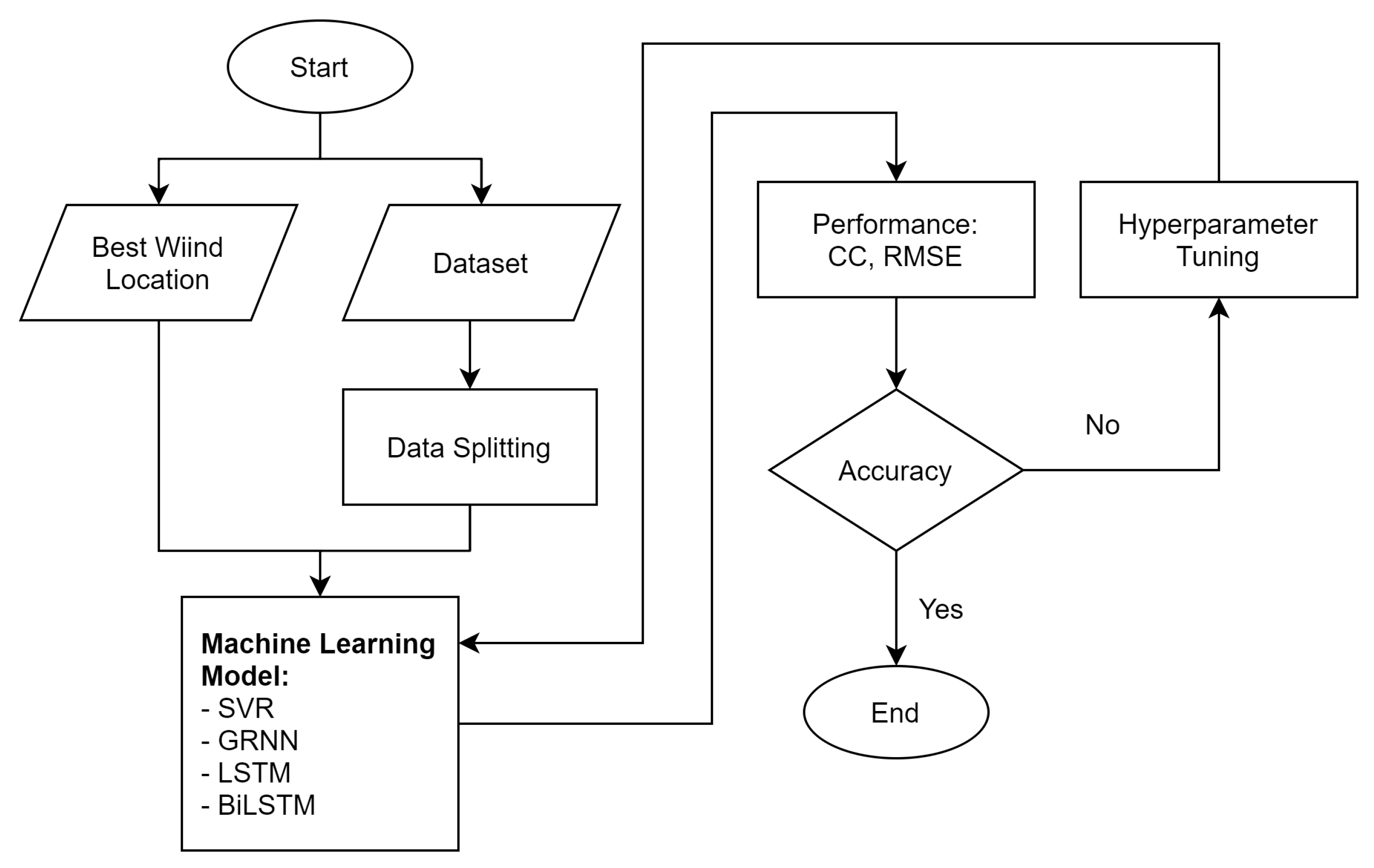
As mentioned previously, we compared the performance of four machine learning models, i.e., the SVR, GRNN, LSTM, and the BiLSTM. Whenever the accuracy of each model was insufficient, we performed hyperparameter tuning for each machine learning model. The procedure of the machine learning optimization can be seen in Figure 13.

After performing hyperparameter tuning for each machine learning model, we obtained the following settings. For the Support Vector Regression (SVR) model, we found that the best parameter settings are with a RBF (radial basis function) kernel, with the parameter $\gamma$ set as “scaled”, an $ϵ$ of $0.05$, and a relative error tolerance of ${10}^{-4}$. For the Generalized Regression Neural Network (GRNN), we found that a spreading parameter of $s=1$ yielded the best performance. For the LSTM model, we used three hidden layers, with the number of nodes at each layer being 512, 16, and 1. The activation function used was sigmoid, and was combined with the tanh function for its recurrent network. In the BiLSTM model, we also had the same configuration as the LSTM model for the number of hidden layers and its corresponding number of nodes, but with a Relu activation function combined with a sigmoid activation function for its recurrent network. For both LSTM and BiLSTM, Adam’s optimizer was used.

Not only did we perform hyperparameter tuning for each machine learning model, but we also investigated the effects of wind features on the resulting wave forecasting accuracy. In the following section, we calculate the machine learning prediction with wind input location based on a spatial correlation with $CC>0.65$, $CC>0.70$, and $CC>0.75$, as shown in Figure 12.

4. Results and Discussion

In this section, we investigate the results of prediction using four machine learning methods, i.e., Support Vector Regression (SVR), the Generalized Regression Neural Network (GRNN), Long Short-Term Memory (LSTM), and Bidirectional LSTM (BiLSTM), with two types of configuration. We investigated the dependency of wave forecasting accuracy regarding the wind feature used for the machine learning input to predict the significant wave height at the study area. Here, we investigate the various configurations of spatially correlated wind features that yield the best performance. Moreover, we investigate the length of training data required to obtain an acceptable forecast accuracy.

4.1. Effect of Spatially Correlated Wind Features

As mentioned in the previous section, it is unclear which wind data locations affect the significant wave height at Jakarta Bay. To investigate the effects of highly spatially correlated wind data with the resulting significant wave height, we performed three scenarios for wind input locations, i.e., wind locations with correlation coefficient values of $CC>0.65$, $CC>0.7$, and $CC>0.75$, as depicted in Figure 12.

To test the effects of the wind location input based on spatial correlation values on the accuracy of wave height prediction, we used 15 years of wind and wave data to train four machine learning methods. Here, we forecasted 14 days using various wind input locations, i.e., wind location with spatial correlation values of $CC>0.65$, $CC>0.7$, and $CC>0.75$, as summarized in

Table 2. Comparison of different methods using selected spatial correlation.

Method	Selected Spatial Correlation	Number of Wind Point Input	CC	RMSE
SVR	CC > 0.65	142	0.38	0.2
	CC > 0.70	88	0.55	0.2
	CC > 0.75	14	0.25	0.21
GRNN	CC > 0.65	142	0.18	0.22
	CC > 0.70	88	0.04	0.24
	CC > 0.75	14	−0.14	0.23
LSTM	CC > 0.65	142	0.95	0.09
	CC > 0.70	88	0.95	0.08
	CC > 0.75	14	0.96	0.08
BiLSTM	CC > 0.65	142	0.87	0.13
	CC > 0.70	88	0.94	0.07
	CC > 0.75	14	0.96	0.06

. Table 2 demonstrates that stronger correlation coefficient values between the wind location point results in a higher accuracy in significant wave height forecasting in terms of CC and RMSE values.

As shown in Table 2, we compared various machine learning methods using spatial data with correlation coefficients greater than 0.65, 0.70, and 0.75. We discovered that using methods based on deep learning produces the best results with high correlation coefficient values and a low root mean square error (RMSE). The SVR method results in the best performance with a spatial correlation of $CC>0.70$, with a correlation coefficient value of 0.55 and an RMSE value of 0.2. In contrast, the GRNN method results in a correlation coefficient value of 0.18 and an RMSE value of 0.22, with the best configuration spatial correlation with CC > 0.65. Two deep learning methods, i.e., the LSTM and BiLSTM, result in a much better performance, with a correlation coefficient value of 0.96 for both methods and RMSE values of 0.08 and 0.07 for the LSTM and BiLSTM methods, respectively. Both deep learning methods produce the best performance, with a spatial correlation configuration where $CC>0.75$. For these two deep learning methods, we can also observe that increasing the number of wind points used as input for each machine learning does not always increase performance.

Using 15 years of training data, we performed predictions using SVR (first row), the GRNN (second row), LSTM (third row), and BiLSTM (fourth row), shown in Figure 14, in 2018. Figure 14 shows that the SVR and GRNN methods show significant error with a lower significant wave height during April–May 2018 and November–December 2018. On the other hand, the LSTM and BiLSTM model results show better performance with high and low significant wave heights. We also compared the results of predictions using SVR, GRNN, LSTM, and BiLSTM in scatter plots, as shown in Figure 15. Figure 15 shows that the results of the significant wave height forecast of both the SVR and GRNN models produce overestimated predictions in some areas, whereas the results of LSTM and BiLSTM show a much better performance. Here, the results of the BiLSTM model produce similar results compared with the testing data.

4.2. Length of Training Data

For a forecasting system based on machine learning, forecast accuracy is highly dependent on the length of the training data used. This subsection investigates the effects of the length of training data in affecting forecast performance. We varied the training data to be 1, 5, 10, and 15 years to forecast 14 and 30 days ahead. We used the BiLSTM model to investigate these scenarios, as summarized in

Table 3. Training data versus testing data variation.

Length Testing Data	Testing Data	CC	RMSE	CPU Time (s)
15 years	14 days	0.96	0.06	3317.02
	30 days	0.92	0.06
10 years	14 days	0.96	0.07	2208.07
	30 days	0.91	0.06
5 years	14 days	0.94	0.08	588.64
	30 days	0.89	0.08
1 year	14 days	0.92	0.1	233.22
	30 days	0.85	0.1

.

Table 3, shows that, to produce a better forecast performance, we require longer training data, i.e., 15 years. We also note that the performance of the forecast model decreases as the forecast period extends, in this case, 30 days ahead. The best performance results were obtained using 15 years of training data to forecast 14 days, with a CC value of 0.96 and an RMSE value of 0.06. Nevertheless, the performance of BiLSTM is also relatively similar using only 10 years of training data, which results in a CC value of 0.96 and an RMSE value of 0.07. In Table 3, we compare the CPU time used for the training process. We used a computer with a a Ryzen-5800H processor, RTX 3060 GPU, and 16 GB of DDR4 RAM. Indeed, a longer period of training data requires more computational time. Qualitatively, the results of the prediction using 15 years of training data to forecast 14 and 30 days are shown in Figure 16. Figure 16 demonstrates that projections for the next 14 and 30 days have reasonable accuracy, indicating that the prediction can track the trend of major significant wave height data.

As seen in Table 3, the results of the prediction using the BiLSTM model with 15 years of training data are not significantly different from the results with 10 years of data. To test the sensitivity of the training data with respect to the resulting accuracy of the prediction, we constructed three scenarios in which we varied the time span of 10 years of training data as 2004–2013, 2006–2015, and 2008–2017, to predict the significant wave height in 2018. The results of these scenarios were compared to forecast 14 and 30 days in 2018.

Table 4. Results of predictions using three different time frames of 10 years of training data.

Training Data	Days to Forecast	CC	RMSE
2004–2013	14	0.95	0.09
	30	0.91	0.07
2006–2015	14	0.95	0.08
	30	0.91	0.07
2008–2017	14	0.96	0.07
	30	0.91	0.07

show the prediction results in terms of CC and RMSE values using three training data frames. The results show that three time frames of training data result in very similar results, with CC values from 0.95 to 0.96 and RMSE values of 0.07 to 0.09, for predictions for 14 days ahead. Note that the training data of 2008–2017 yield the best performance in terms of CC and RMSE. Nevertheless, the results using the other time frames of training data, 2004–2013 and 2006–2015, also do not give a much worse performance. These facts might indicate climate variation in the study area, i.e., Jakarta Bay, but it is insignificant.

4.3. Sensitivity of Wave Location to Forecast

The results of significant wave height (Hs) forecasting in the previous subsection are a prediction of Hs at the observation point in Jakarta Bay, as indicated in Figure 7. Nevertheless, the geometry of Jakarta Bay shows a complex sheltered area. The accuracy of predicting Hs at one location compared to another location near the coastline might be different. In this subsection, we also investigate the accuracy of prediction in other point locations in Jakarta Bay, as indicated in Figure 17. Here, the observation point is denoted by $P0$, whereas other locations are numbered as $P1,P2,\cdots ,P15$. To check the sensitivity of prediction accuracy concerning Hs points, we performed predictions using the BiLSTM model for points at northern locations, i.e., $P3,P6,P9,P12$, and $P15$, and for points at southern locations, i.e., $P1,P4,P7,P10$, and $P13$. For the northern points, we used a Spatial Correlation (SC) where $CC>0.75$. Meanwhile, for the southern points, we used an SC where $CC>0.70$ since, for these points, there are no CC values larger than $0.75$.

Results of the prediction for these points are summarized in

Table 5. Results of significant wave height prediction at various locations.

Wave Point	Selected Spatial Correlation	Number of Wind Point Input	Days to Forecast	CC	RMSE
P0	SC > 0.75	14	14	0.96	0.06
			30	0.92	0.06
P1	SC > 0.70	14	14	0.96	0.05
			30	0.93	0.05
P3	SC > 0.75	13	14	0.96	0.07
			30	0.91	0.08
P4	SC > 0.70	19	14	0.97	0.06
			30	0.92	0.06
P6	SC > 0.75	13	14	0.96	0.08
			30	0.91	0.08
P7	SC > 0.70	14	14	0.97	0.07
			30	0.93	0.06
P9	SC > 0.75	13	14	0.96	0.07
			30	0.93	0.07
P10	SC > 0.70	9	14	0.97	0.07
			30	0.93	0.06
P12	SC > 0.75	11	14	0.97	0.07
			30	0.94	0.07
P13	SC > 0.70	3	14	0.96	0.06
			30	0.92	0.07
P15	SC > 0.75	4	14	0.97	0.08
			30	0.94	0.07

. Although the number of wind points to be included as features in the machine learning models varies, i.e., from 4 to 19, the results of the Hs prediction are relatively consistent both for the southern and northern points. For 14-day forecasting, the results at all locations are relatively consistent with CC values from 0.96 to 0.97 and RMSE values from 0.06 to 0.08.

4.4. Forecasting of Tp and Mean Wave Direction

In the previous subsection, we extensively discussed predicting significant wave height Hs. The peak wave period Tp and mean wave direction are other important wave properties. Two main steps were performed when designing a significant wave height forecasting system. Firstly, we built a spatial correlation map from the wind field and Hs to determine the best locations for wind points. Secondly, we performed machine learning training for wind data with significant wave height target data at the selected wind locations. We also used a similar methodology to predict Tp and mean wave direction. We performed the prediction of Tp and mean wave direction using the BiLSTM model with 15 years of training data, as in the prediction of Hs in the previous subsection. Here, we also used the wave information at the observation point as shown in Figure 7. Results of the prediction for 14 and 30 days ahead are shown in Figure 18 for peak period Tp and in Figure 19 for mean wave direction. From Figure 18, the predicted Tp shows relatively good results, but at some crests and throughs, the results of the prediction are overestimated. Nevertheless, the results of the predicted Tp can follow the target data accurately.

The prediction of the mean wave direction, as shown in Figure 19, qualitatively showS A better performance than the prediction of Tp. Results of the Tp and mean wave direction prediction are summarized in

Table 6. Results of the prediction of the peak wave period (Tp) and the mean wave direction using the BiLSTM model.

Parameter to Forecast	Days to Forecast	CC	RMSE
Tp	14	0.83	0.83
	30	0.77	0.74
Mean Wave Direction	14	0.92	12.92
	30	0.90	13.16

, in terms of CC and RMSE. As indicated qualitatively, the predictions of the mean wave direction are better than the predictions of Tp. Note that the unit for RMSE in Tp prediction is in second (s), whereas that in mean wave direction is in degrees (${}^{\circ }$).

5. Conclusions

In this paper, we introduced a novel approach to designing a wave forecasting system based on combined high-resolution numerical wave simulation with a deep learning model, i.e., BiLSTM, to forecast significant wave height in an environment with a complex geometry, such as a coastal area with many islands. To that aim, we generated training data for the deep learning model using continuous numerical simulation using the SWAN model with two nested domains. We compared the SWAN simulation results with available wave observation data at Jakarta Bay, Java Sea, Indonesia, to validate the SWAN simulation results. The obtained training data were then used as training data for the deep learning method. To obtain the best possible wind feature as input for the deep learning model, we calculated spatial correlation values between the wind data at all locations in the Southeast Asia region and the significant wave height at the observation location in Jakarta Bay. Our investigation concludes that using wind input locations with a high spatial correlation improves forecast performance. In our case, wind locations with spatial correlation values with significant wave height data in Jakarta Bay of $CC>0.75$ yielded the best forecast performance, with a correlation coefficient value of 0.96 and an RMSE value of 0.06. We also investigated the effect of the length of the training data in forecast performance. From a numerical experiment, we concluded that training data of 15 years yields the best performance compared with training data of a shorter period of time, even though results with 10 years of training data also yielded very similar results. In addition to significant wave height Hs, we also performed predictions of the peak wave period Tp and the mean wave direction. Since the characteristics of Tp are quite different from Hs, we obtained a CC value of 0.83 for predicting 14 days, whereas the mean wave direction results in a better performance with a CC value of 0.92. To predict Tp, more appropriate machine learning models can be investigated, since Tp characteristics are very different from Hs and mean wave direction.

References

1. Wu, M.; Stefanakos, C.; Gao, Z. Multi-Step-Ahead Forecasting of Wave Conditions Based on a Physics-Based Machine Learning (PBML) Model for Marine Operations. J. Mar. Sci. Eng. 2020, 8, 992. [Google Scholar] [CrossRef]
2. Shamshirband, S.; Mosavi, A.; Rabczuk, T.; Nabipour, N.; Chau, K.W. Prediction of significant wave height; comparison between nested grid numerical model, and machine learning models of artificial neural networks, extreme learning and support vector machines. Eng. Appl. Comput. Fluid Mech. 2020, 14, 805–817. [Google Scholar] [CrossRef]
3. Chen, D.; Liu, F.; Zhang, Z.; Lu, X.; Li, Z. Significant Wave Height Prediction based on Wavelet Graph Neural Network. In Proceedings of the 2021 IEEE 4th International Conference on Big Data and Artificial Intelligence (BDAI), Qingdao, China, 2–4 July 2021; pp. 80–85. [Google Scholar]
4. Ali, M.; Prasad, R.; Xiang, Y.; Deo, R.C. Near real-time significant wave height forecasting with hybridized multiple linear regression algorithms. Renew. Sustain. Energy Rev. 2020, 132, 110003. [Google Scholar] [CrossRef]
5. Ali, M.; Prasad, R. Significant wave height forecasting via an extreme learning machine model integrated with improved complete ensemble empirical mode decomposition. Renew. Sustain. Energy Rev. 2019, 104, 281–295. [Google Scholar] [CrossRef]
6. Tür, R. Maximum wave height hindcasting using ensemble linear-nonlinear models. Theor. Appl. Climatol. 2020, 141, 1151–1163. [Google Scholar] [CrossRef]
7. Zhang, X.; Li, Y.; Gao, S.; Ren, P. Ocean Wave Height Series Prediction with Numerical Long Short-Term Memory. J. Mar. Sci. Eng. 2021, 9, 514. [Google Scholar] [CrossRef]
8. O’Donncha, F.; Zhang, Y.; Chen, B.; James, S.C. An integrated framework that combines machine learning and numerical models to improve wave-condition forecasts. J. Mar. Syst. 2018, 186, 29–36. [Google Scholar] [CrossRef] [Green Version]
9. Group, T.W. The WAM model—A third generation ocean wave prediction model. J. Phys. Oceanogr. 1988, 18, 1775–1810. [Google Scholar] [CrossRef] [Green Version]
10. Booij, N.; Ris, R.; Holthuijsen, L. A third-generation wave model for coastal regions, Part I, Model description and validation. J. Geophys. Res. 1999, 104, 7649–7656. [Google Scholar] [CrossRef] [Green Version]
11. Tolman, H.L. A third-generation model for wind waves on slowly varying, unsteady, and inhomogeneous depths and currents. J. Phys. Oceanogr. 1991, 21, 782–797. [Google Scholar] [CrossRef]
12. Bingölbali, B.; Akpınar, A.; Jafali, H.; Van Vledder, G.P. Downscaling of wave climate in the western Black Sea. Ocean Eng. 2019, 172, 31–45. [Google Scholar] [CrossRef]
13. Atan, R.; Nash, S.; Goggins, J. Development of a nested local scale wave model for a 1/4 scale wave energy test site using SWAN. J. Oper. Oceanogr. 2017, 10, 59–78. [Google Scholar] [CrossRef] [Green Version]
14. Jain, P.; Deo, M.; Latha, G.; Rajendran, V. Real time wave forecasting using wind time history and numerical model. Ocean Model. 2011, 36, 26–39. [Google Scholar] [CrossRef]
15. Rizianiza, I.; Aisjah, A.S. Prediction of Significant Wave Height in The Java Sea Using Artificial Neural Network. In Proceedings of the 2015 International Seminar on Intelligent Technology and Its Applications (ISITIA), Surabaya, Indonesia, 20–21 May 2015; pp. 5–9. [Google Scholar]
16. Nikoo, M.R.; Kerachian, R.; Alizadeh, M.R. A fuzzy KNN-based model for significant wave height prediction in large lakes. Oceanologia 2018, 60, 153–168. [Google Scholar] [CrossRef]
17. Zubier, K.M. Using an artificial neural network for wave height forecasting in the Red Sea. Indian J. Geo Mar. Sci. 2020, 49, 184–191. [Google Scholar]
18. Wang, T.; Gao, S.; Xu, J.; Li, Y.; Li, P.; Ren, P. Correcting predictions from oceanic maritime numerical models via residual learning. In Proceedings of the 2018 OCEANS-MTS/IEEE Kobe Techno-Oceans (OTO), Kobe, Japan, 28–31 May 2018; pp. 1–4. [Google Scholar]
19. Elbisy, M.S. The Use of Group Method of Data Handling and Multilayer Perceptron Neural Network for the Prediction of Significant Wave Height. Am. Sci. Res. J. Eng. Technol. Sci. (ASRJETS) 2019, 60, 174–183. [Google Scholar]
20. Liu, T.; Zhang, Y.; Qi, L.; Dong, J.; Lv, M.; Wen, Q. WaveNet: Learning to predict wave height and period from accelerometer data using convolutional neural network. In IOP Conference Series: Earth and Environmental Science; IOP Publishing: Tokyo, Japan, 2019; p. 012001. [Google Scholar]
21. Callens, A.; Morichon, D.; Abadie, S.; Delpey, M.; Liquet, B. Using Random forest and Gradient boosting trees to improve wave forecast at a specific location. Appl. Ocean Res. 2020, 104, 102339. [Google Scholar] [CrossRef]
22. Yu, T.; Wang, J. A Spatiotemporal Convolutional Gated Recurrent Unit Network for Mean Wave Period Field Forecasting. J. Mar. Sci. Eng. 2021, 9, 383. [Google Scholar] [CrossRef]
23. Hersbach, H.; Bell, B.; Berrisford, P.; Hirahara, S.; Horányi, A.; Muñoz-Sabater, J.; Nicolas, J.; Peubey, C.; Radu, R.; Schepers, D.; et al. The ERA5 global reanalysis. Q. J. R. Meteorol. Soc. 2020, 146, 1999–2049. [Google Scholar] [CrossRef]
24. Dhanistha, W.L.; Atmoko, R.; Juniarko, P.; Akbar, R. Prediction of Significant Wave Height Using Neural Network in the Java Sea (North of Surabaya). Appl. Mech. Mater. 2017, 862, 72–77. [Google Scholar] [CrossRef]
25. Juliani, V.; Adytia, D.; Adiwijaya. Wave Height Prediction based on Wind Information by using General Regression Neural Network, study case in Jakarta Bay. In Proceedings of the 2020 8th International Conference on Information and Communication Technology (ICoICT), Yogyakarta, Indonesiam, 24–26 June 2020; pp. 1–5. [Google Scholar] [CrossRef]
26. Ris, R.; Booij, N.; Holthuijsen, L. A third-generation wave model for coastal regions: 2. Verification. J. Geophys. Res. 1999, 104, 7667–7681. [Google Scholar] [CrossRef]
27. James, S.C.; Zhang, Y.; O’Donncha, F. A machine learning framework to forecast wave conditions. Coast. Eng. 2018, 137, 1–10. [Google Scholar] [CrossRef] [Green Version]
28. Hochreiter, S.; Schmidhuber, J. Long short-term memory. Neural Comput. 1997, 9, 1735–1780. [Google Scholar] [CrossRef] [PubMed]
29. Fan, S.; Xiao, N.; Dong, S. A novel model to predict significant wave height based on long short-term memory network. Ocean Eng. 2020, 205, 107298. [Google Scholar] [CrossRef]
30. Zhang, A.; Lipton, Z.C.; Li, M.; Smola, A.J. Dive into deep learning. arXiv 2021, arXiv:2106.11342. [Google Scholar]
31. Schuster, M.; Paliwal, K. Bidirectional recurrent neural networks. IEEE Trans. Signal Process. 1997, 45, 2673–2681. [Google Scholar] [CrossRef] [Green Version]
32. Zhao, R.; Yan, R.; Wang, J.; Mao, K. Learning to monitor machine health with convolutional bi-directional LSTM networks. Sensors 2017, 17, 273. [Google Scholar] [CrossRef] [PubMed]
33. Graves, A.; Schmidhuber, J. Framewise phoneme classification with bidirectional LSTM networks. In Proceedings of the 2005 IEEE International Joint Conference on Neural Networks, Montreal, QC, Canada, 31 July–4 August 2005; Volume 4, pp. 2047–2052. [Google Scholar] [CrossRef] [Green Version]
Figure 1. Architecture of Long Short Term Memory (LSTM).
Fluids 07 00039 g001
Figure 2. Architecture of Bidirectional LSTM (BiLSTM).
Fluids 07 00039 g002
Figure 3. Flowchart of wave data generation.
Fluids 07 00039 g003
Figure 4. Snapshot of the wind field (upper plot) and the resulting significant wave height from the SWAN simulation (lower plot) in Domain-1.
Fluids 07 00039 g004
Figure 5. Similar to Figure 4 for Domain-2.
Fluids 07 00039 g005
Figure 6. Similar to Figure 4 for Domain-3.
Fluids 07 00039 g006
Figure 7. Location of wave observations at Jakarta Bay, Java Sea.
Fluids 07 00039 g007
Figure 8. Comparison between the significant wave height results from the SWAN simulation with wave observation data, waves from ECMWF ERA-5, and waves from GFS-NOAA, in Jakarta Bay.
Fluids 07 00039 g008
Figure 9. Flowchart for exploratory data.
Fluids 07 00039 g009
Figure 10. Spatial Correlation (SC) between wind speed data with significant wave height at the observation point in Jakarta Bay.
Fluids 07 00039 g010
Figure 11. Similar as in Figure 10, for the northwestern area of the Java Sea.
Fluids 07 00039 g011
Figure 12. Spatial Correlation (SC) between the wind field and the wave data at the observation point, where C C > 0.65 (upper left plot), C C > 0.70 (upper right plot), and C C > 0.75 (lower plot).
Fluids 07 00039 g012
Figure 13. Flowchart for machine learning optimization.
Fluids 07 00039 g013
Figure 14. Results of significant wave height forecasting at the observation point in Jakarta Bay using the SVR, GRNN, LSTM, and BiLSTM methods.
Fluids 07 00039 g014
Figure 15. Scatter plot of the results of the significant wave height predictions with the SVR (upper left plot), GRNN (upper right plot), LSTM (lower left plot), and BiLSTM (lower right plot) methods with testing data at the observation location in Jakarta Bay, Java Sea.
Fluids 07 00039 g015
Figure 16. Prediction and testing significant wave height using BiLSTM for 15 years training.
Fluids 07 00039 g016
Figure 17. Locations of wave predictions in Jakarta Bay.
Fluids 07 00039 g017
Figure 18. Results of peak wave period (Tp) prediction for 14 (upper plot) and 30 days (lower plot) ahead using the BiLSTM model with 15 years of training data.
Fluids 07 00039 g018
Figure 19. Results of the prediction of the mean wave direction for 14 (upper plot) and 30 days (lower plot) ahead using the BiLSTM model with 15 years of training data.
Fluids 07 00039 g019