Numerical Study for Unsteady Waves Generated by Flow over a Permeable Wavy Bed

Abstract

In this paper, we formulate a numerical model to study unsteady waves generated by fluid flow over a permeable wavy bed. The model is derived from boundary value problems using potential theory. We solve the model numerically using a finite difference method. As a result, we found that the flow over a porous layer generates wave disturbed by bumps on the porous layer. The simulation also showed that the wave profile shifts from the permeable bed. The results of this study can be incorporated into the design of submerged artificial and natural breakwaters.

1. Introduction

Most coastal protection structures consist of permeable beds or porous media that cause the waves passing through them to be reflected or dissipated. A structure is declared efficient if it is able to maximize dissipation and minimize reflections. Some examples of the use of porous mediums in coastal defense structures include submerged porous breakwaters, which can be formed by natural and artificial coral reefs. Besides their beauty and utility as marine habitats, coral reefs are also able to reduce beach erosion [1,2,3].

Several studies on flows over a porous layer can be found in the literature. For instance, the numerical scheme of Liu et al. [4] was validated using data from simple experiments on liquid flows through different porous mediums types. Carotenuto and Minale [5] experimentally investigated the velocity profile of a fluid undergoing simple shear above a porous medium. Kim, Cho, and Choi [6] analyzed the experimental result with theoretical results calculated using Darcy’s Law and Forchheimer’s equation. However, experiments are costly. Consequently, recent studies have focused on the use of mathematical modeling to investigate flows over a porous media. Examples of researchers who have studied flows over a porous layer using Navier–Stokes equations include Liu et al. [4], who constructed a numerical scheme based on Navier–Stokes equations, Bruneau and Mortazavi [7] who build a numerical model based on Navier–Stokes equations, and Cimolin and Discacciati [8], who compared the Navier–Stokes/Forchheimer, Navier–Stokes/Darcy, and penalization models. Models for flow over permeable beds have also been formulated with the shallow water equations (SWEs) as their base. These are known for their simplicity. For example, Magdalena et al. [9] studied wave interaction with submerged porous mediums, Wiryanto [10] analyzed wave propagation over a submerged breakwater for monochromatic and solitary waves, and Wiryanto [11] studied fluid disturbances caused by the uneven surface of a porous medium. There are trade-offs involved when choosing between these approaches. Models based on Navier–Stokes equations are more computationally expensive [12] and SWEs are less precise for solving problems with high complexity [13].

In this paper, we derive a model for unsteady waves generated by a flow over a permeable wavy bed based on potential theory and Darcy’s law. Potential theory is then used to build a model similar to a Boussinesq-type equation. This model was chosen because of its ability to describe complex cases and handle dispersion waves [13,14]. Additionally, its linear approximation is in good agreement with nonlinear results [15]. This model has also been widely used to investigate wave phenomena, such as in the works of Kennedy et al. [16], who simulated wave run-up on a conical island, and Schäffer et al. [17], who simulated waves breaking in shallow water. Then, a numerical scheme is constructed to solve the governing equations using a second-order forward-time center-space finite difference method. This method is chosen because can be solved explicitly and is relatively simple, meanings that it has a low computational cost [18]. This scheme can be used to observe the effects of model parameters and the surface bed profile on fluid motion.

The rest of the paper is structured as follows. Problem formulation is presented in Section 2. The numerical scheme is provided in Section 3. The numerical result is described in Section 4, and the conclusions are presented in Section 5.

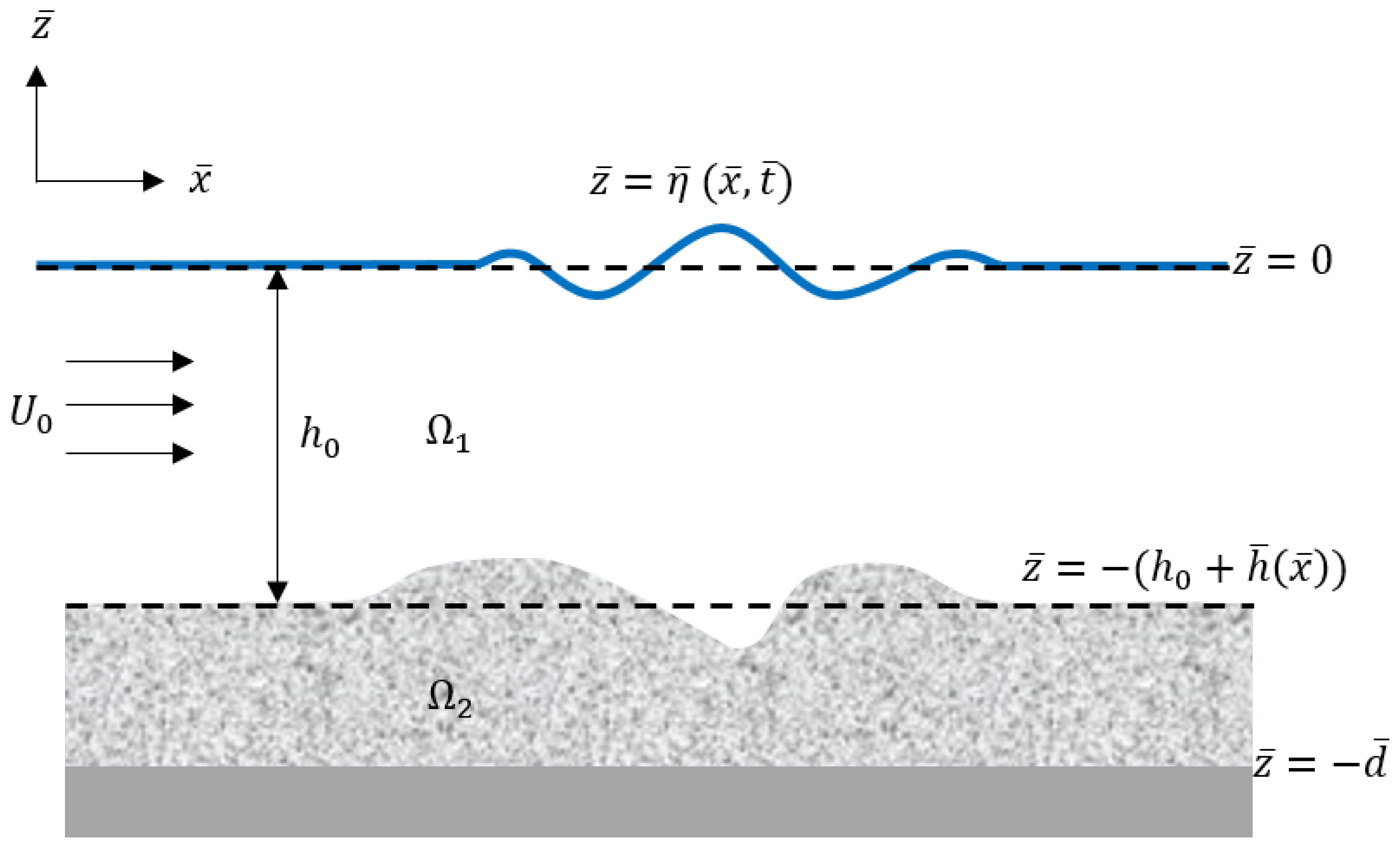
2. Problem Formulation

In this section, a model of fluid flows over a porous layer with permeability K (as illustrated in Figure 1) is formulated. The fluid has a depth of $h_0$ and flows with velocity $U_0$. The variables involved in this model are $\overline{x}$ and $\overline{z}$, with $\overline{z}=0$ measured in still water. We use $\overline{\eta }(x,t)$ to denote the surface elevation. The surface of the porous medium follows $\overline{z}=-(h_0+\overline{h}\left(x\right))$, and the solid bottom of the bed is constant at $\overline{z}=-d$. We use $\varphi$ and ${\varphi }^{\prime }$ to represent the potential functions in the upper region ${\mathrm{\Omega }}_1$ and the lower region ${\mathrm{\Omega }}_2$, respectively.

From the conservation of mass for an incompressible flow in ${\mathrm{\Omega }}_1$, the Laplace equation is derived.

$${\overline{\varphi }}_{\overline{x}\overline{x}}+{\overline{\varphi }}_{\overline{z}\overline{z}}=0,-(h_0+\overline{h}\left(\overline{x}\right))<\overline{z}<\overline{\eta }(\overline{x},\overline{t}).$$

(1)

Kinematic and dynamic conditions on the free surface $\overline{\eta }(\overline{x},\overline{t})$ allow the following to be obtained

$${\overline{\eta }}_{\overline{t}}+{\overline{\varphi }}_{\overline{x}}{\overline{\eta }}_{\overline{x}}-{\overline{\varphi }}_{\overline{z}}=0,\overline{z}=\overline{\eta },$$

(2)

$${\overline{\varphi }}_{\overline{t}}+\frac{1}{2}({\overline{\varphi }}_{\overline{x}}^2+{\overline{\varphi }}_{\overline{z}}^2)+g\overline{\eta }=\frac{1}{2}{U}_0^2,\overline{z}=\overline{\eta },$$

(3)

with g as the gravitational acceleration. The expression on the right hand side of Equation (3) represents the constant initial disturbance. We can observe the fluid moving from one medium to another on the interface between ${\mathrm{\Omega }}_1$ and ${\mathrm{\Omega }}_2$. This motion follows the Bernoulli equation

$${\overline{\varphi }}_{\overline{t}}+\frac{1}{2}({\overline{\varphi }}_{\overline{x}}^2+{\overline{\varphi }}_{\overline{z}}^2)+g\overline{z}+\frac{p^{\prime }}{\rho }=\frac{1}{2}{U}_0^2,\overline{z}=-(h_0+\overline{h}\left(\overline{x}\right)),$$

(4)

where $p^{\prime }$ and $\rho$ are pressure on the porous medium and fluid density, respectively. Darcy’s Law for porous media Mizumura [19] states

$${\overline{\varphi }}^{\prime }=-K(\rho g\overline{z}+p^{\prime })/v,$$

(5)

where v is viscosity. Substituting this to Equation (4) gives us

$${\overline{\varphi }}_{\overline{t}}+\frac{1}{2}({\overline{\varphi }}_{\overline{x}}^2+{\overline{\varphi }}_{\overline{z}}^2)-\frac{v}{K\rho }{\overline{\varphi }}^{\prime }=\frac{1}{2}{U}_0^2,\overline{z}=-(h_0+\overline{h}\left(\overline{x}\right)).$$

(6)

Since the kinematic condition on the interface between two mediums satisfies continuity, the kinematic condition of both mediums must be equal. Hence, we have

$${\overline{\varphi }}_{\overline{x}}{\overline{h}}_{\overline{x}}+{\overline{\varphi }}_{\overline{z}}={\overline{\varphi }}_{\overline{x}}^{\prime }{\overline{h}}_{\overline{x}}+{\overline{\varphi }}_{\overline{z}}^{\prime }.$$

(7)

Due to continuity, the porous media also satisfy the Laplace equation

$${\overline{\varphi }}_{\overline{x}\overline{x}}^{\prime }+{\overline{\varphi }}_{\overline{z}\overline{z}}^{\prime }=0,-d<\overline{z}<-(h_0+\overline{h}\left(\overline{x}\right)).$$

(8)

It follows from the kinematic condition at the bottom of the porous medium that

$${\overline{\varphi }}_{\overline{z}}^{\prime }=0,\overline{z}=-d.$$

(9)

Then we normalize the scaled variables by defining $x=\overline{x}/\lambda ,y=\overline{y}/h_0,t=\overline{t}\sqrt{g{h}_0}/\lambda ,$$\eta =\overline{\eta }/a,\varphi =\overline{\varphi }{h}_0/\lambda U_{0}a,{\varphi }^{\prime }={\overline{\varphi }}^{\prime }{h}_0/\lambda U_{0}a,h=\overline{h}/a,d=\overline{d}/h_0$. Here, a and $lambda$ denote the wave amplitude and wavelength, respectively. Furthermore, we define $\overline{\varphi }$ as

$$\overline{\varphi }=U_0\overline{x}+\overline{\mathrm{\Phi }}$$

This represents the uniform stream and its perturbation. Transforming to the normalized form and dividing by $\frac{\lambda U_{0}a}{h_0}$ yields

$$\varphi =\frac{h_0}{a}x+\mathrm{\Phi }.$$

(10)

By using the chain rule, we obtain

$${\overline{\varphi }}_{\overline{x}}=\frac{U_{0}a}{h_0}(\frac{h_0}{a}+{\mathrm{\Phi }}_x);{\overline{\varphi }}_{\overline{x}\overline{x}}=\frac{U_{0}a}{h_0\lambda }{\mathrm{\Phi }}_{xx},$$

(11)

$${\overline{\varphi }}_{\overline{z}}\frac{\lambda U_{0}a}{h_0^2}{\mathrm{\Phi }}_z;{\overline{\varphi }}_{\overline{z}\overline{z}}=\frac{\lambda U_{0}a}{h_0^3}{\mathrm{\Phi }}_{zz},$$

(12)

$${\overline{\varphi }}_{\overline{t}}=\frac{U_{0}a\sqrt{g{h}_0}}{h_0}{\mathrm{\Phi }}_t.$$

(13)

Substituting Equations (11) and (12) to Equation (1) and dividing by $\frac{\lambda U_{0}a}{h_0^3}$ yields

$${\mu }^2{\mathrm{\Phi }}_{xx}+{\mathrm{\Phi }}_{zz}=0,$$

(14)

with $\mu =\frac{h_0}{\lambda }$ representing the dispersive effect. Similarly, we have

$${\mu }^2{\varphi }_{xx}^{\prime }+{\varphi }_{zz}^{\prime }=0.$$

(15)

Now we want to denote Equations (2) and (3) in their normalized forms. The differentiation of $\overline{\eta }$ can be obtained by the chain rule and expressed as

$${\overline{\eta }}_{\overline{x}}=\frac{a}{\lambda }{\eta }_x,$$

(16)

$${\overline{\eta }}_{\overline{t}}=\frac{a\sqrt{g{h}_0}}{\lambda }{\eta }_t.$$

(17)

Substitute Equations (11), (12), (16), and (17) to Equation (2) and divide it by $\frac{a\lambda \sqrt{g{h}_0}}{h_0^2}$, we have

$${\mu }^2{\eta }_t+F{\mu }^2{\eta }_x+Fϵ{\mu }^2{\mathrm{\Phi }}_x{\eta }_x-F{\mathrm{\Phi }}_z=0,z=ϵ\eta ,$$

(18)

where $F=U_0/\sqrt{g{h}_0}$ and $ϵ=a/h_0$ express the Froude number and the non-linear effect, respectively. Substituting Equations (11)–(13) into Equation (3) and dividing by $ga$, we obtain

$$F{\mathrm{\Phi }}_t+\frac{1}{2}{F}^2(2{\mathrm{\Phi }}_x+ϵ{\mathrm{\Phi }}_x^2+\frac{ϵ}{{\mu }^2}{\mathrm{\Phi }}_z^2)+\eta =0,z=ϵ\eta .$$

(19)

We can transform the dynamic condition on the interface of two mediums by substituting Equations (11)–(13) to Equation (6) and dividing by $\frac{U_{0}a\sqrt{g{h}_0}}{h_0}$. Hence, we obtain

$${\mathrm{\Phi }}_t+\frac{1}{2}(2F{\mathrm{\Phi }}_x+Fϵ{\mathrm{\Phi }}_x^2+\frac{ϵ}{{\mu }^2}{\mathrm{\Phi }}_y^2)-\frac{F}{R}{\varphi }^{\prime }=0,z=-(1+ϵh\left(x\right)),$$

(20)

where $R=U_0\rho K/\left(v\lambda \right)$ is the Reynolds number. The derivative of h is obtained using the chain rule.

$${\overline{h}}_{\overline{x}}=\frac{a}{\lambda }{h}_x,$$

This can be substituted into Equation (7) and divided by $\frac{\lambda U_{0}a}{h_0^2}$ to obtain

$${\mu }^2{h}_x+{\mu }^2ϵ{\mathrm{\Phi }}_x{h}_x+{\mathrm{\Phi }}_z={\mu }^2ϵ{\varphi }_x^{\prime }{h}_x+{\varphi }_z^{\prime },z=-(1+ϵh\left(x\right)).$$

(21)

Meanwhile, we transform the kinematic condition at the bottom of porous medium (9) by noting that ${\overline{\varphi }}_{\overline{z}}^{\prime }=\frac{\lambda U_{0}a}{h_0^2}{\varphi }_z^{\prime }$ and divide it by $\frac{\lambda U_{0}a}{h_0^2}$. So, we have

$${\varphi }_z^{\prime }=0,z=-d.$$

(22)

Assume that $\mathrm{\Phi }$ and ${\varphi }^{\prime }$ can be expressed as

$$\mathrm{\Phi }={\mathrm{\Phi }}_0+ϵ{\mathrm{\Phi }}_1+{ϵ}^2{\mathrm{\Phi }}_2+\dots$$

(23)

$${\varphi }^{\prime }={\varphi }^{\prime \left(0\right)}+ϵ{\varphi }^{\prime \left(1\right)}+{ϵ}^2{\varphi }^{\prime \left(2\right)}+\dots$$

(24)

Using $ϵ={\mu }^2$, we then solve for the potential function $\mathrm{\Phi }$ and ${\varphi }^{\prime }$ from Equation (14) with the condition Equations (15) and (19) with condition Equation (22). By analyzing those equations order by order, we obtain

$$\mathrm{\Phi }={\mathrm{\Phi }}_0(x,t)+ϵ(-\frac{1}{2}{{\mathrm{\Phi }}_0}_{xx}{z}^2+(\frac{{\eta }_t}{F}+{\eta }_x)z+C(x,t)),$$

(25)

$${\varphi }^{\prime }={\varphi }^{\prime \left(0\right)}(x,t)+ϵ(-\frac{1}{2}{{\varphi }_{xx}^{\prime }}^{\left(0\right)}{(z+d)}^2+C^{\prime }(x,t)),$$

(26)

where ${\mathrm{\Phi }}_0,{\varphi }^{\prime \left(0\right)},C,$ and $C^{\prime }$ are functions of x and t. Here, $ϵ$ is assumed to be very small. By substituting Equations (25) and (26) to Equations (19)–(21), we can then obtain

$$F{{\mathrm{\Phi }}_0}_t(x,t)+F^2{{\mathrm{\Phi }}_0}_x(x,t)+\eta =0,$$

(27)

$${{\mathrm{\Phi }}_0}_t(x,t)+F{{\mathrm{\Phi }}_0}_x(x,t)-\frac{F}{R}{\varphi }^{\prime \left(0\right)}(x,t)=0,$$

(28)

$$h_x+{\mathrm{\Phi }}_{0xx}+\frac{{\eta }_t}{F}+{\eta }_x={{\varphi }_{xx}^{\prime }}^{\left(0\right)}(1-d).$$

(29)

Taking the second derivative of Equation (28) with respect to x and multiplying it by $R(1-d)/F$, we have

$$\frac{R(1-d)}{F}{{\mathrm{\Phi }}_0}_{xxt}+R(1-d){{\mathrm{\Phi }}_0}_{xxx}={{\varphi }_{xx}^{\prime }}^{\left(0\right)}(1-d).$$

(30)

By eliminating Equation (29) and (30) and multiplying both sides by F, we obtain

$${\eta }_t+F({\eta }_x+{\mathrm{\Phi }}_{0xx}+h_x)=(1-d)R({\mathrm{\Phi }}_{0xxt}+F{\mathrm{\Phi }}_{0xxx})$$

(31)

Now we define the depth-average velocity

$$u=\frac{1}{1+ϵ\eta +ϵh}{\int }_{-1-ϵh}^{ϵ\eta }{\mathrm{\Phi }}_{x}dz.$$

(32)

Substituting Equation (25) into Equation (32) and ignoring the terms with the $ϵ$ multiplier yields

$$u\approx {{\mathrm{\Phi }}_0}_x.$$

(33)

By approximating u with ${{\mathrm{\Phi }}_0}_x$ in Equation (31), we find

$${\eta }_t+F({\eta }_x+u_x+h_x)=(1-d)R(u_{xt}+F{u}_{xx}).$$

(34)

This is then followed by taking the derivative of Equation (27) and expressing it in u form

$$F{u}_t+F^2{u}_x+{\eta }_x=0$$

(35)

Therefore, we have Equations (34) and (35) as our model. The effect of the porous layer can be seen on the right hand side of Equation (34), with the absorption ability of the porous medium defined by R and d. These cannot be observed separately since they appear as one coefficient. When the porous medium is absent, the model can be obtained by setting $R=0$, yielding a model that agrees with the linear equations in Wiryanto [20].

3. Numerical Method

Here, we want to determine $\eta$ and u in the model (34) and (35) numerically. We solve these equations using forward time centered space as illustrated in Figure 2. We define $\Delta x$ and $\Delta t$ as the spatial and time steps, respectively. Their values are chosen to fulfill the stability condition in (Appendix A). Other CFL criteria for SWE have also been derived by Fennema and Chaudhry [21] and Gharangik and Chaudhry [22]. Now, we denote $h\left(x\right)=h_j$, $\eta (x,t)={\eta }_j^n$ and $u(x,t)=u_j^n$, with $x=j\Delta x$ for $j=0,1,2,\dots$ and $t=n\Delta t$ for $n=0,1,2,\dots$

By taking the derivative of Equation (35) and substitute it to Equation (34), we obtain

$${\eta }_t+F({\eta }_x+u_x+h_x)=\frac{(d-1)R}{F}{\eta }_{xx}.$$

(36)

Discretizing Equations (35) and (36) yields

$$u_j^{n+1}=u_j^n-\Delta tF\frac{u_{j+1}^n-u_{j-1}^n}{2\Delta x}-\frac{\Delta t}{F}\frac{{\eta }_{j+1}^n-{\eta }_{j-1}^n}{2\Delta x},$$

(37)

$$\begin{array}{c}\hfill {\eta }_j^{n+1}={\eta }_j^n-\Delta tF\frac{{\eta }_{j+1}^n-{\eta }_{j-1}^n+u_{j+1}^n-u_{j-1}^n+h_{j+1}-h_{j-1}}{2\Delta x}\\ \hfill +\Delta t\frac{(d-1)R}{F}\frac{({\eta }_{j+1}^n+{\eta }_{j-1}^n-2{\eta }_j^n)}{\Delta x^2}.\end{array}$$

(38)

We set ${\eta }_0^n=0$ and $u_0^n=0$ to express that our left-hand boundary is relatively far from the disturbance. Since we need ${\eta }_{j+1}^n$ and $u_{j+1}^n$ to determine $\eta$ and u in the next time step, we can obtain the values of these quantities just beyond the right-hand boundary by extrapolating the right-hand boundary values of $\eta$ and u. The boundary is an absorbing boundary. We take ${\eta }_j^0=0$ and $u_j^0=0$ as the initial condition, which is undisturbed uniform flow.

4. Numerical Result

After formulating the numerical scheme, it is implemented to calculate the elevation $\eta$ and velocity u for several values of F, R, d and $h\left(x\right)$. The calculations here use $\Delta x=0.1$ and $\Delta t=0.001$ which complies with the stability condition in Appendix A. Most simulations run from $t=0$ to $t=30$, as the fluid remains relatively steady during this time period.

First, we want to see how the Froude number F affects the wave elevation. In order to do that, we simulate the elevation for different values of t in the same plane, which shifted upward for larger t, for various F. In this case, we take a look at the permeable layer with sinusoidal bump

$$h\left(x\right)=-0.1sin\left(\pi \right(x-45)/10)$$

at $x\in [45,55]$. In Figure 3, we observe the surface elevation using $F=0.2$, $F=0.6$, $F=1$, and $F=1.4$ with the same values of $R(d-1)=0.3$. We can see that the wave with the larger F has a larger amplitude. The wave propagating to the left also moves at a slower speed. We can see that the slope of the line connecting the maximum point on the surface elevation at any time increases with the value of F. In fact, for $F=1$ and $F=1.4$, we have no waves propagating to the left and the wave remains above the bump. This is referred to as a supercritical condition. This result agrees with Mizumura [23], who analyzed the water surface profiles over a wavy bed, and along a wavy side wall using the Laplace equation.

Here, we observe the effect of the porous layer by considering the surface elevation for different values of $R(d-1)$. The effect of the porous layer appears in the diffusion term ${\eta }_{xx}$, which dampens the waves. The waves should be increasingly damped as the diffusion term’s influence increases. In Figure 4, we compare the surface elevation at $\eta (x,30)$ corresponding to $R(d-1)=0$ (impermeable bed), $0.3$, and 1, for $F=0.2$ and 1. This result agrees with Wiryanto [11], as in Figure 5. In the cited study, a fourth-order numerical scheme is constructed and then solved using the Gauss–Seidel method. We are able to simulate the model using a lower order model and solve it explicitly.

For comparison with different bed types, we simulate waves propagating over permeable beds with different amplitudes, wave numbers, and more bumps. From Figure 6, we can conclude that the elevation of the waves formed will increase as the amplitude of the permeable bed’s bumps increases.

Meanwhile, Figure 7 shows that different wave numbers cause the wave elevation steepness to vary.

To investigate the effect of more bumps, we define the following function to represent the permeable bed’s surface

$$h\left(x\right)=-0.2sin\left(\pi \right(x-15)/10)$$

at $x\in [15,75]$. We set supercritical flow $F=1.5$, $R(d-1)=2.0$ to produce waves moving towards the right-hand boundary. The simulation results can be seen in Figure 8.

By running the simulation for a longer period of time, we found that simulating wave elevation over this surface shifts the elevation, as shown in Figure 9. Higher values of $R(d-1)$ coincide with larger shifts. This result agrees with Mizumura [19], Wiryanto [20], and Wiryanto [24], who used series expansions to extract the first and second order terms for steady flow over a wavy permeable bed problem. It also agrees with the results of Iwasa and Kennedy [25], who derived it using shear flow theory, and Ho and Gelhar [26] who analyzed it theoretically based on potential flow theory and the linear Darcy equation.

5. Conclusions

In this paper, we derived a linear unsteady model for surface waves generated by a flow passing over a permeable wavy bed. The forward-time centered-space finite difference method has been applied to solve the model numerically. This solution is then used to observe the propagation of the fluid surface waves, allowing the effects of the Froude number and the characteristics of the porous medium on wave generation to be observed. Higher Froude numbers produce larger wave amplitudes and when $F\ge 1$, a supercritical condition is reached where no waves propagate to the left. Meanwhile, the damping effect increases with the characteristic value of the porous media $R(d-1)$, leading to smaller wave amplitudes. These results are also in accordance with the physical properties of waves. Steady waves were obtained by running simulations for longer simulation times using this second order numerical scheme. It was also found that the permeable bed’s presence causes the wave profile to shift, which is confirmed by previous studies. This implies that the model successfully describes the physical phenomenon of waves generated by flow over a porous layer. Furthermore, this model’s simplicity and ease of use means that it can be used in studying and developing various wave phenomena when permeable media.

References

1. Reguero, B.G.; Beck, M.W.; Agostini, V.N.; Kramer, P.; Hancock, B. Coral reefs for coastal protection: A new methodological approach and engineering case study in Grenada. J. Environ. Manag. 2018, 210, 141–161. [Google Scholar] [CrossRef] [PubMed]
2. Ferrario, F.; Beck, M.W.; Storlazzi, C.D.; Micheli, F.; Shepard, C.C.; Airoldi, L. The effectiveness of coral reefs for coastal hazard risk reduction and adaptation. Nat. Commun. 2014, 5, 3794. [Google Scholar] [CrossRef] [PubMed]
3. Zhao, M.; Zhang, H.; Zhong, Y.; Jiang, D.; Liu, G.; Yan, H.; Wang, R. The Status of Coral Reefs and Its Importance for Coastal Protection: A Case Study of Northeastern Hainan Island, South China Sea. Sustainability 2019, 11, 4354. [Google Scholar] [CrossRef] [Green Version]
4. Liu, P.L.F.; Lin, P.; Chang, K.A.; Sakakiyama, T. Numerical modeling of wave interaction with porous structures. J. Waterw. Port Coast. Ocean. Eng. 1999, 125, 322–330. [Google Scholar] [CrossRef]
5. Carotenuto, C.; Minale, M. Shear flow over a porous layer: Velocity in the real proximity of the interface via rheological tests. Phys. Fluids 2011, 23, 063101. [Google Scholar] [CrossRef]
6. Kim, D.; Cho, E.; Choi, C. An experimental study on fluid flow characteristics of superposed porous and fluid layers. Korean J. Chem. Eng. 1994, 11, 190–197. [Google Scholar] [CrossRef]
7. Bruneau, C.-H.; Mortazavi, I. Numerical modelling and passive flow control using porous media. Comput. Fluids 2008, 37, 488–498. [Google Scholar] [CrossRef]
8. Cimolin, F.; Discacciati, M. Navier–Stokes/Forchheimer models for filtration through porous media. Appl. Numer. Math. 2013, 72, 205–224. [Google Scholar] [CrossRef] [Green Version]
9. Magdalena, I.; Pudjaprasetya, S.R.; Wiryanto, L.H. Wave interaction with emerged porous structure. Adv. Appl. Math. Mech. 2014, 6, 680–692. [Google Scholar] [CrossRef]
10. Wiryanto, L.H. Wave propagation passing over a submerged porous breakwater. J. Eng. Math. 2011, 70, 129–136. [Google Scholar] [CrossRef]
11. Wiryanto, L.H. Unsteady waves generated by flow over a porous layer. IAENG Int. J. Appl. Math. 2010, 40, 233–238. [Google Scholar]
12. Audusse, E.; Steinstraesser, J.C.; Emerald, L.; Heinrich, P.; Paris, A.; Parisot, M. Comparison of models for the simulation of landslide generated Tsunamis. ESAIM Proc. Surv. 2021, 70, 14–30. [Google Scholar] [CrossRef]
13. Hervouet, J.M.; Jankowski, J. Comparing numerical simulations of free surface flows using non-hydrostatic Navier–Stokes and Boussinesq equations. In Proceedings of the 4th Conference on Hydroinformatics, Iowa City, IA, USA, 16–18 October 2000. [Google Scholar]
14. Yincan, Y.; Xianghua, L.; Guofu, P.; Qitong, L.; Zhenye, Z.; Dujuan, L.; Xiaoling, C.; Yanji, W.; Junren, C.; Taojun, H.; et al. Chapter 5: Sea Earthquake and Earthquake Tsunami in Marine Geo-Hazards in China (edited by Yincan et al.); Elsevier: Amsterdam, The Netherlands, 2017. [Google Scholar]
15. Forbes, L.K.; Schwartz, L.W. Free-surface flow over a semicircular obstruction. J. Fluid Mech. 1982, 114, 299–314. [Google Scholar] [CrossRef]
16. Kennedy, B.; Chen, Q.; Kirby, J.T.; Dalrymple, R.A. Boussinesq Modeling Of Wave Transformation, Breaking, And Runup I: 1D. J. Waterw. Port Coast. Ocean. Eng. 2002, 126, 39–47. [Google Scholar] [CrossRef] [Green Version]
17. Schäffer, H.A.; Madsen, P.A.; Deigaard, R. A Boussinesq model for waves breaking in shallow water. Coast. Eng. 1993, 20, 185–202. [Google Scholar] [CrossRef]
18. Chu, W.; Willis, R. An Explicit Finite Difference Model for Unconfined Aquifers. Groundwater 1984, 22, 728–734. [Google Scholar] [CrossRef]
19. Mizumura, K. Free surface flow over permeable wavy bed. Hydraul. Eng. 1998, 124, 955–962. [Google Scholar] [CrossRef]
20. Wiryanto, L.H.; Anwarus, S. Monochromatic waves over permeable bed. In Proceeding of the 5th Asian Mathematical Conference, Kuala Lumpur, Malaysia, 22–26 June 2009; pp. 617–622. [Google Scholar]
21. Fennema, R.J.; Chaudhry, M.H. Simulation of one-dimensional dam-break flows. J. Hydraul. Res. 1987, 25, 41–51. [Google Scholar] [CrossRef]
22. Gharangik, M.A.; Chaudhry, M.H. Numerical simulation of hydraulic jump. J. Hydraul. Eng. ASCE 1991, 117, 1195–1211. [Google Scholar] [CrossRef]
23. Mizumura, K. Free-surface profile of open-channel flow with wavy boundary. J. Hydraul. Eng. 1995, 121, 533–539. [Google Scholar] [CrossRef]
24. Wiryanto, L.H. Wave propagation over a submerged bar. ITB J. Sci. A 2010, 42, 81–90. [Google Scholar] [CrossRef] [Green Version]
25. Iwasa, Y.; Kennedy, J.F. Free surface shear flow over a wavy bed. J. Hydraul. Div. 1968, 94, 431–454. [Google Scholar] [CrossRef]
26. Ho, R.T.; Gelhar, L.W. Turbulent flow with wavy permeable boundaries. J. Fluid Mech. 1973, 58, 403–414. [Google Scholar] [CrossRef]
Figure 1. Illustration.
Fluids 07 00009 g001
Figure 2. Scheme of forward time centered space.
Fluids 07 00009 g002
Figure 3. Waves generated by flow over a permeable bed for subcritical flow: (a). F = 0.2 , (b). F = 0.3 , supercritical flow: (c). F = 1.0 , (d). F = 1.4 ; R ( d 1 ) = 0.3 .
Fluids 07 00009 g003
Figure 4. η ( x , 30 ) for R ( d 1 ) = 0 (red), R ( d 1 ) = 0.3 (green), and 1.0 (blue), using (a). F = 0.2 (subcritical flow) and (b). F = 1.0 (supercritical flow).
Fluids 07 00009 g004
Figure 5. Simulation using second order (blue) and fourth order (red) numerical scheme using (a). R ( d 1 ) = 0.3 and F = 0.2 (subcritical flow), (b). R ( d 1 ) = 1 and F = 0.2 (subcritical flow), (c) R ( d 1 ) = 0.3 and F = 1 (supercritical flow), and (d). R ( d 1 ) = 1 and F = 1 (supercritical flow) at t = 30 .
Fluids 07 00009 g005
Figure 6. Waves generated by flow over a permeable bed with F = 1 (supercritical flow) and R ( d 1 ) = 0.3 for the surface of the permeable h ( x ) = 0.1 sin ( π ( x 45 ) / 10 ) (blue), h ( x ) = 0.2 sin ( π ( x 45 ) / 10 ) (red), and h ( x ) = 0.3 sin ( π ( x 45 ) / 10 ) (green) at x [ 45 , 55 ] .
Fluids 07 00009 g006
Figure 7. Waves generated by flow over a permeable bed with F = 1 (supercritical flow) and R ( d 1 ) = 0.3 for the surface of the permeable h ( x ) = 0.1 sin ( π ( x 45 ) / 10 ) (blue), h ( x ) = 0.1 sin ( π 2 ( x 45 ) / 10 ) (red), h ( x ) = 0.1 sin ( π 3 ( x 45 ) / 10 ) (green) at x [ 45 , 55 ] .
Fluids 07 00009 g007
Figure 8. Waves generated by flow over a permeable bed for F = 1.5 (supercritical flow) and R ( d 1 ) = 2.0 .
Fluids 07 00009 g008
Figure 9. The steady waves (solid curve) compared with the interface profile (dash lines) of the wavy bed for (a) R ( d 1 ) = 2.0 , (b) 3.0 , and (c) 5.0 .
Fluids 07 00009 g009
Publisher’s Note: MDPI stays neutral with regard to jurisdictional claims in published maps and institutional affiliations.