Abstract
The demand for wind energy harvesting has grown significantly to mitigate the global challenges of climate change, energy security, and zero carbon emissions. Various methods to maximize wind power efficiency have been proposed. Notably, neural networks have shown large potential in improving wind power efficiency. In this paper, we provide a review of attempts to maximize wind power efficiency using neural networks. A total of three neural-network-based strategies are covered: (i) neural-network-based turbine control, (ii) neural-network-based wind farm control, and (iii) neural-network-based wind turbine blade design. In the first topic, we introduce neural networks that control the yaw of wind turbines based on wind prediction. Second, we discuss neural networks for improving the energy efficiency of wind farms. Last, we review neural networks to design turbine blades with superior aerodynamic performances.
1. Introduction
Concerns surrounding climate change continue to grow and related treaties have been signed. For example, in COP26 (26th UN Climate Change Conference of the Parties), most developed countries agreed to abolish traditional coal power generation and halt new construction. This agreement aims to control rises in temperature by achieving a “net zero” balance of carbon emission and absorption by 2050 [1]. Therefore, it is crucial to minimize, or eliminate if possible, carbon generation during energy harvesting processes.
Wind is a ubiquitous source of energy that can be harvested without carbon emission. Wind turbines (WT) are utilized to convert the kinetic energy of wind to usable forms of energy (e.g., electricity). Accordingly, the installation of WTs has significantly increased owing to their negligible carbon emission [2,3]. However, the number of WTs that can be installed is limited due to concerns related to species protection and geopolitical and supply risks [2]. Indeed, the high production and maintenance costs associated with WTs also present one of the main factors warranting consideration before installation [4]. Therefore, with limits in increasing the number of WTs, it is essential to maximize the zero-carbon energy generation from wind by further optimizing the energy efficiency of turbines.
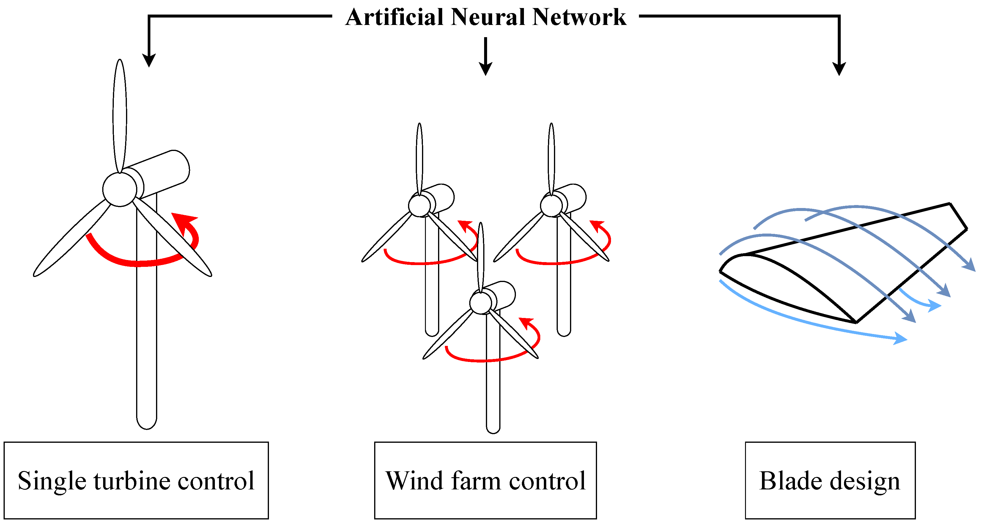
The energy efficiency of WTs depends on the interactions between atmospheric flow and wind blades. Atmospheric flow—a turbulent boundary layer flow with moving boundaries and external energy sources—is highly non-linear. The interaction between turbulent flow and wind blades is also non-linear, and depends on factors such as wind direction, angle of attack, and blade geometry. Hence, designing WTs requires simulations or experiments that involve full interactions between turbulent atmospheric flow and turbine blades [5,6]. Therefore, significant challenges exist in optimizing the energy efficiency of WTs. Recently, several studies have employed machine learning (ML) models to optimize WT energy efficiency [7,8] or to maintain WTs [9,10,11] efficiently. In particular, neural networks (NN), a type of ML model, have shown significant potential to be utilized for wind energy harvesting. This is due to the state-of-the-art performance of NNs in learning non-linear patterns, such as the chaotic patterns in atmospheric flows. Studies on improving the energy efficiency of WTs using deep NNs can be categorized as follows (see Figure 1):
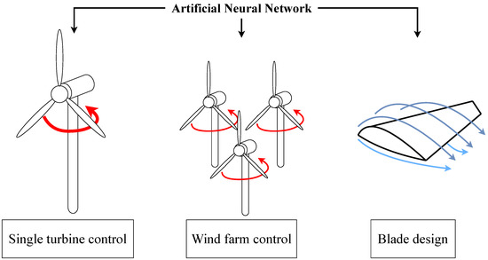
Figure 1.
Schematic of our categorization.
- NN-based single turbine control
- NN-based wind farm control
- NN-based wind blade design
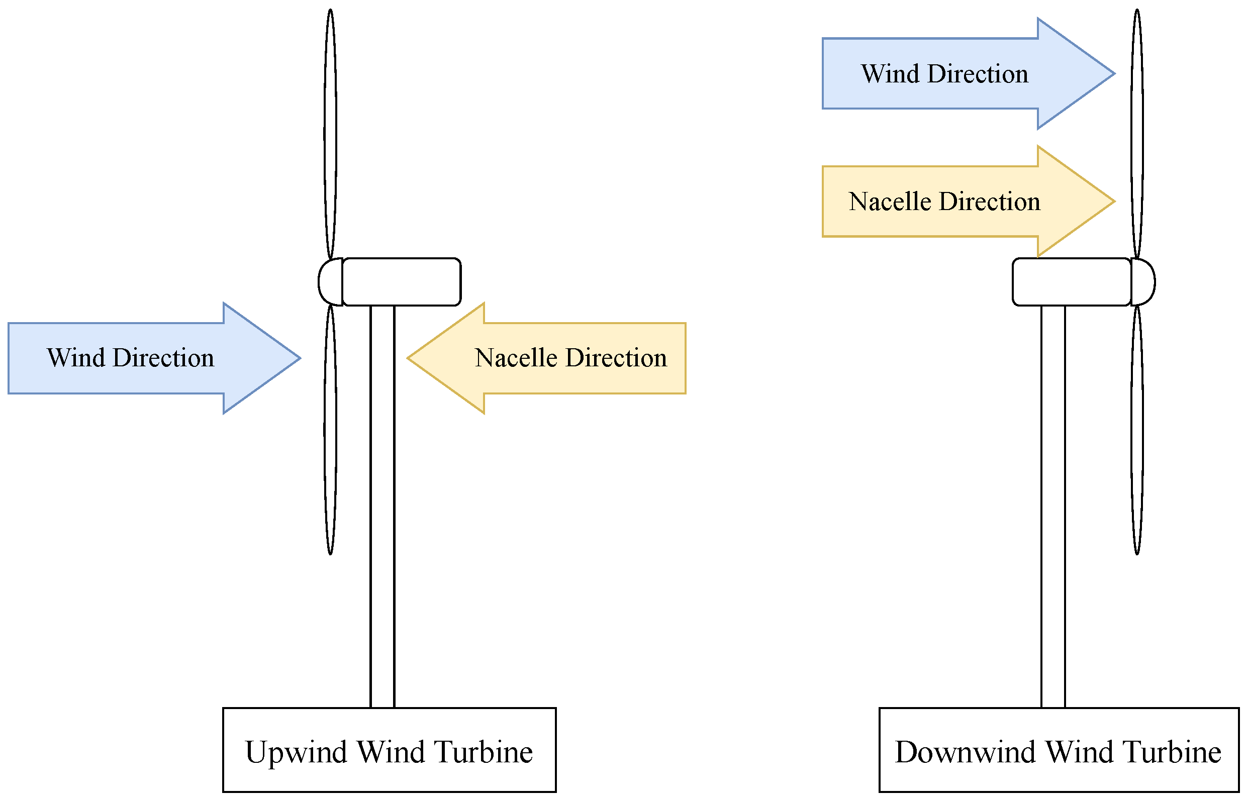
We discuss the recent developments of deep NNs for improving the energy efficiency of WTs in the three categories above. This paper is organized as follows: NN-based turbine control is discussed in Section 2. Section 3 investigates approaches for NN-based wind farm control. NN-based blade design methods are introduced in Section 4, followed by concluding remarks in Section 5. All WTs covered in this paper are horizontal-axis upwind wind turbines (see Appendix A for more details about upwind wind turbines).
2. NN-Based Single Turbine Control
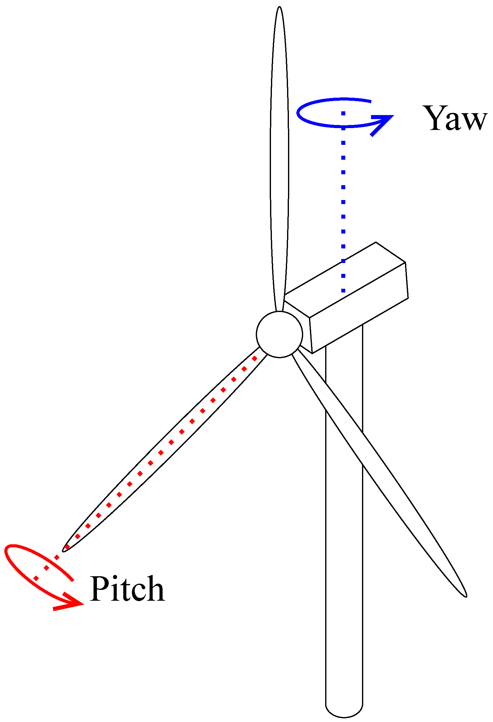
Atmospheric flows around WTs are turbulent, leading to chaotic changes in harvestable winds in space and time. Therefore, a WT must constantly respond to the surrounding atmospheric flow to stabilize power production and minimize fatigue damage [4,12]. Accordingly, modern WTs are designed with pitch- and yaw-angle control systems (Figure 2). A turbine pitch-control system controls the pitch of wind blades. A turbine yaw-control system controls the WT’s nacelle position (i.e., turbine face direction) to react to the chaotic surrounding flows properly [4].
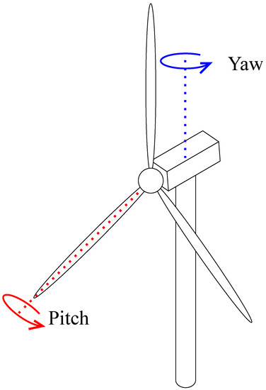
Figure 2.
Schematic of yaw and pitch control of a wind turbine.
A turbine pitch-control system generally aims to prevent WT damage caused by large aerodynamic loads due to excessively high-speed winds with large turbulent fluctuations [4,12,13,14,15,16]. This can be achieved by controlling the pitch angle of wind blades, leading to a change in angle of attacks [12]. Newer pitch-control systems employ electrical or hydraulic drive systems with a proportional–integral–derivative (PID) controller or a proportional–integral (PI) controller [13,14]. Since NN-based pitch-control systems generally aim to prevent turbine damage, they are not further reviewed in this paper. In contrast to pitch-control systems, turbine yaw-control systems aim to maximize energy production. Controlling the yaw angle is one of the most effective methods for maximizing wind energy efficiency. Generally, the maximum wind energy can be harvested when the turbine’s nacelle position is aligned with the surrounding wind velocity vector. One approach for this could be to align the position continuously with the guidance of sensors. However, conventional wind turbines rotate with a slow angular velocity of almost /s [17,18,19]. Due to the slow angular velocity, changes in the surrounding wind direction can occur during rotation, making it challenging to maintain the desired alignment. Continuous movement would also lead to faster wear. In addition, according to Yang et al. [20], the wind data measured by a turbine’s sensor differs from the true wind conditions. Therefore, it is suggested to use future wind directions for improving wind turbine performance. However, forecasting wind velocity presents a significant challenge due to the turbulent characteristics of atmospheric flow. Recently, researchers have attempted to control the yaw angle using NNs for wind forecasting. Details of such methods are discussed below.
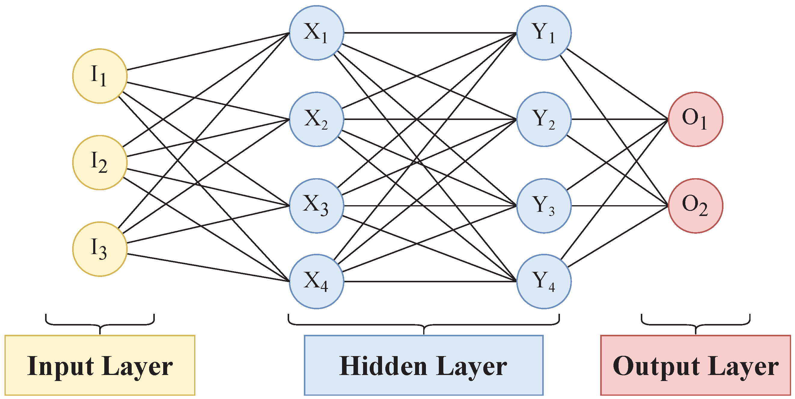
The idea to control yaw angles of WTs based on wind prediction was proposed by Hure et al. [17]. The authors developed a yaw controller using information from short-term wind predictions and reported an improvement in power generation. The wind prediction was performed using a multi-layer perceptron (MLP) type NN developed by Kani and Ardehali [21] and Ðalto et al. [22]. Consequently, researchers have actively employed MLPs for predicting wind [23,24,25]. Figure 3 provides an example of such an MLP. In this example, the input layer has three neurons (, , ), each hidden layer has four neurons (, …, ; , …, ), and the final layer has two neurons (, ).

Figure 3.
Schematic of an MLP model.
NNs are reported to display state-of-the-art performance in learning non-linear data. They can be considered non-linear functions that transform input information into predictions. Let and be two connected layers with and neurons, with and . The information in X is then transported to the next layer Y by a matrix calculation with non-linear activation () as:
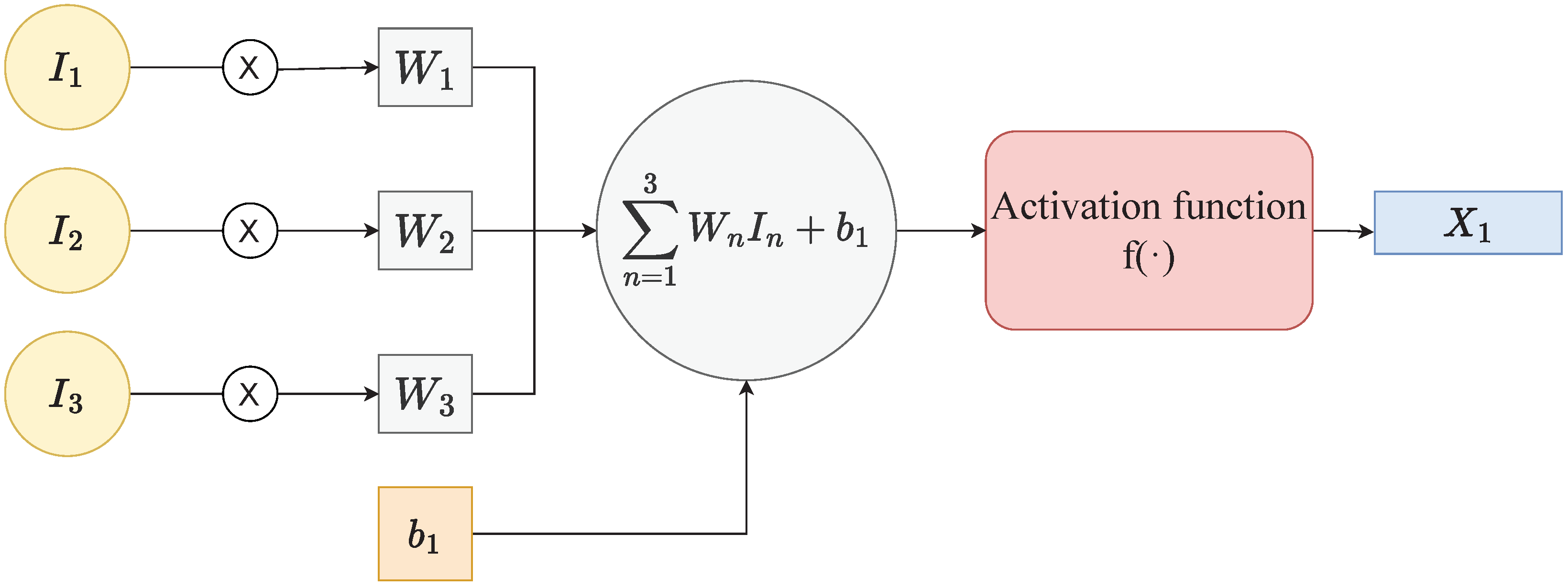
where W is the weight matrix connecting the layers X and Y, and b is a bias vector. The process is illustrated in Figure 4 for the computation of from Figure 3. Note that and . The objective of NNs is to learn the best weights W and biases b that best model the mapping between input and output data. The activation function () enables NNs to learn non-linear relationships between input and output data [26]. Note that a leaky-Rectified linear unit (ReLU) activation function, a variation of the ReLU activation function [27], is one of the most representative activation functions, and is defined as
where x is an arbitrary tensor, is typically a value between [28,29]. The input information is transported to the output layer by repeating the process in Equation (1). The final layer of the NN outputs the prediction. Subsequently, the errors between the model prediction and ground truth data (i.e., labeled data) are computed to evaluate the model prediction. Generally, the mean squared error (MSE) is utilized to evaluate errors in regression results. The MSE is the mean value of squared errors defined as:
where and y are the predicted and labeled values, respectively. The weights and biases are updated with respect to a minimization of the calculated error.
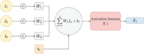
Figure 4.
Schematic of a neuron shown for the computation of from Figure 3.
More recently, owing to the success of long short-term memory (LSTM) NNs, some studies have used LSTMs for predicting the wind direction [30,31]. An LSTM is proposed to compensate for a recurrent neural network (RNN)’s difficulty in learning long-term time-series data.
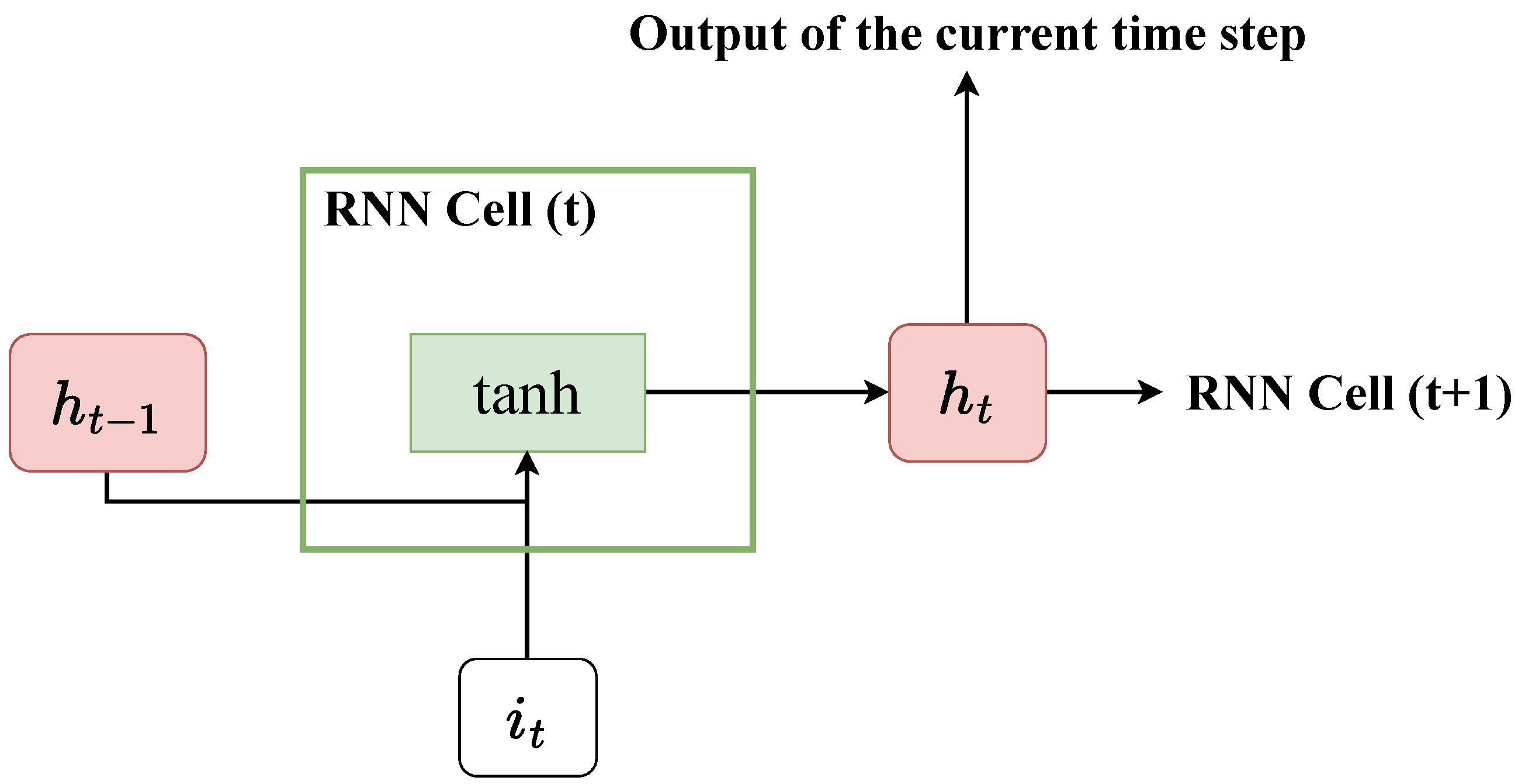
An RNN predicts sequential values by inputting the previous time step’s hidden state () and the current time step’s input () to a gate with a hyperbolic tangent function (see Figure 5). The current time step’s output () functions as the next time step’s hidden state. This process can be seen as having a short-term memory of past values.
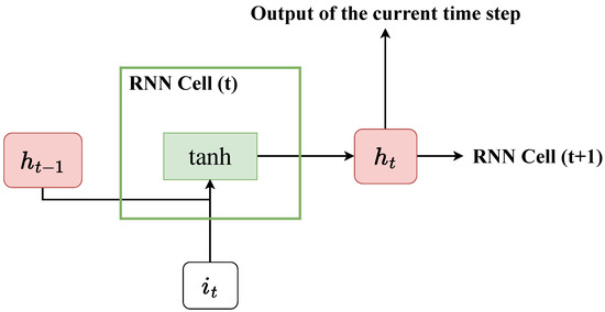
Figure 5.
Schematic of a basic RNN model.
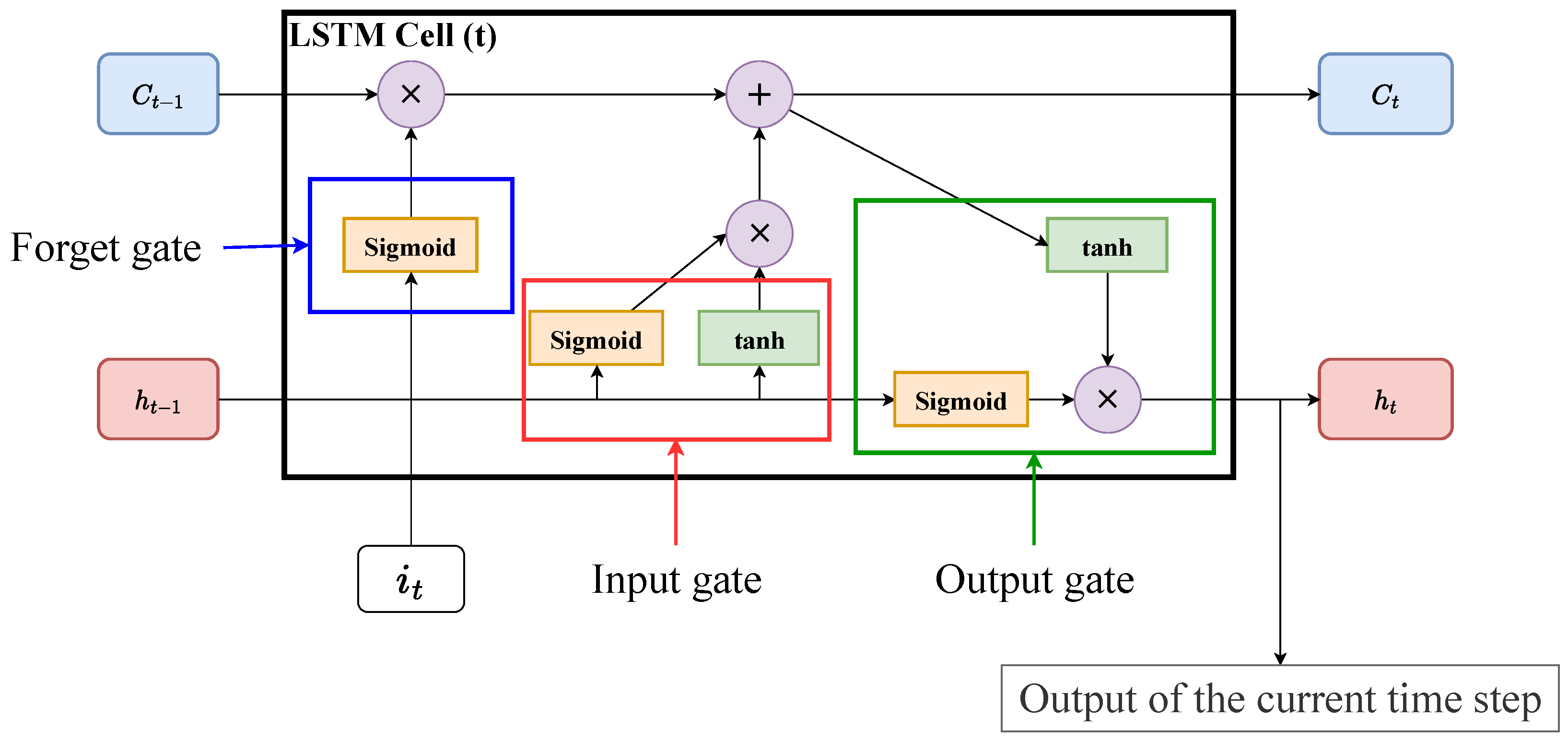
Figure 6 provides a detailed illustration of an LSTM that is known to outperform RNNs in learning sequential correlations for the sake of the long- and short-term memories. Unlike RNNs, an LSTM contains three gates:
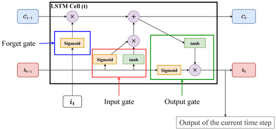
Figure 6.
Schematic of an LSTM model.
- Forget gate: The forget gate calculates the element-wise product of the () values of the current input () and previous hidden state (). The forget gate affects the current cell state ().
- Input gate: The input gate computes the element-wise product of the and values of and . The result of the input gate is used together with the result of the forget gate to compute .
- Output gate: The output gate performs the element-wise product between the value of and values of and . As a result, the current hidden state () can be calculated.
The cell states and hidden states in an LSTM cell function as long- and short-term memories, respectively.
Using an LSTM, Chen et al. [18] successfully controlled the yaw angle of a wind turbine. Their LSTM model was trained with wind data acquired by a light detection and ranging (LiDAR) system. The input of their model was the wind LiDAR data, while the outputs were the desired yaw angle and actuation time that can cope with future wind. Using the LSTM model, energy efficiency improved by approximately and a reduction of 5.3% in travel distance in yaw direction were reported.
In addition to LSTM, convolutional neural networks (CNN) are also well known for their capability of learning spatio-temporal data [32,33,34,35]. Few studies have integrated yaw-control systems with recent CNNs to advance wind prediction. In this paper, we also review CNN-based wind prediction methods that could improve turbine yaw-control systems.
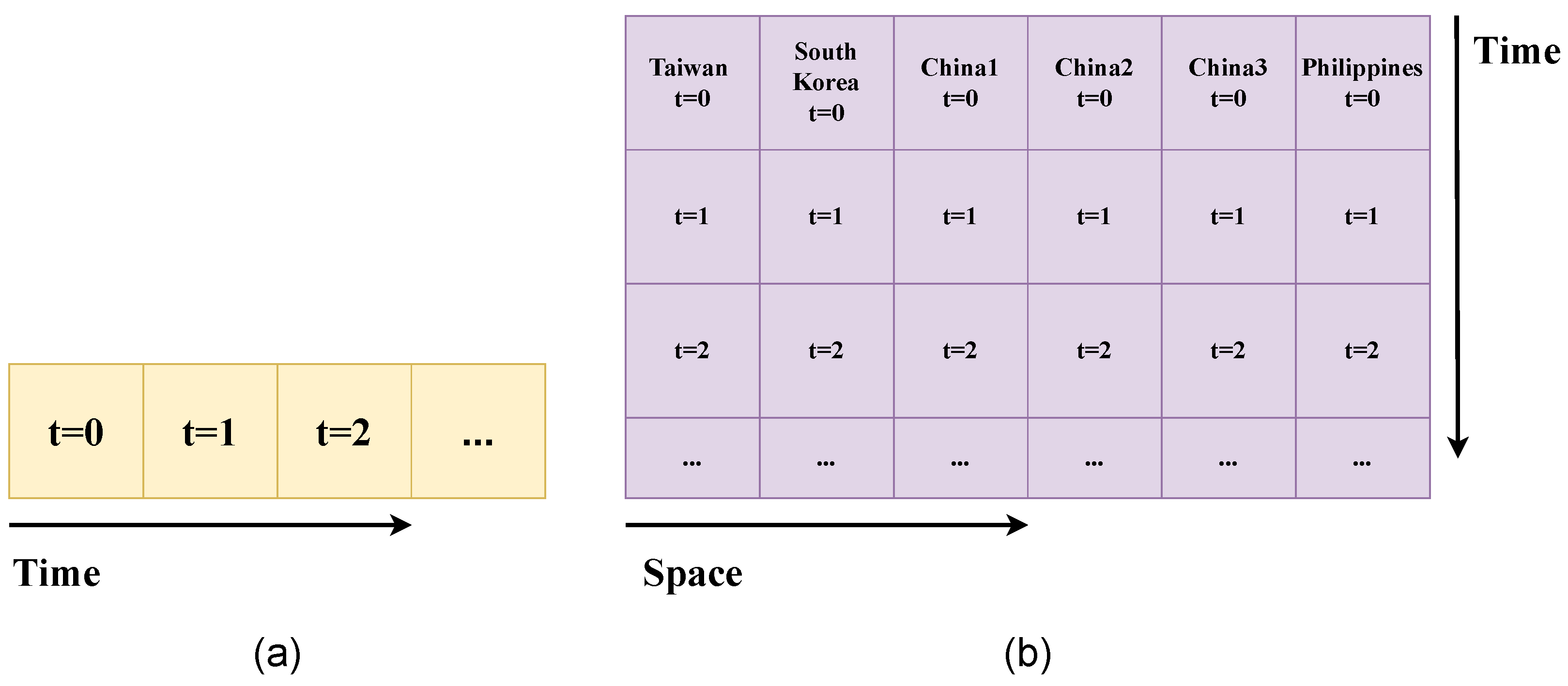
CNNs with different dimensionalities have been exploited for wind prediction, such as one-, two-, and three-dimensional CNNs. First, one-dimensional (1D) CNNs are capable of learning one-dimensional time-sequential data (Figure 7a). For example, Harbola and Coors [36] developed a 1D CNN that predicts temporal wind data in the Netherlands and in the German city of Stuttgart. The authors pre-processed the wind velocity data by categorizing it into 11 classes with different ranges (lower range, upper range):
where and are the mean and standard deviation of the wind velocity data, and .
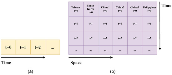
Figure 7.
Schematic of input data of 1D (a) and 2D (b) CNNs for wind prediction.
Their CNNs aim to predict the class of wind velocity on a future occasion. They developed a 1D CNN that predicts the future wind speed and velocity based on the past 25-h wind velocity data within 30-min time-intervals. This 1D CNN model successfully classified the range of the future wind speed and direction at 96.8%, 99.7%, respectively, for Stuttgart, and 98.8%, 99.4%, respectively, for the Netherlands.
However, the underlying physics of atmospheric flow is not one-dimensional. It is a function related to both space and time. Therefore, physically, the inclusion of spatial information should improve the performance of wind prediction. Two-and three-dimensional CNNs can learn spatial correlations in wind data. Hong and Satriani [37] used a two-dimensional (2D) CNN model to predict wind at a target site in Taiwan, using additional wind data from six other regions in South Korea, China, and the Philippines. In total, 78 h of past wind data at the seven sites, which can be rearranged to a array, were used as the input of their 2D CNN model (Figure 7b). Their model showed a lower root mean square error (RMSE), normalized mean square error (NMSE), and mean absolute percentage error (MAPE) compared to an LSTM and an MLP. The errors are defined as:
where y is the ground truth value, is the predicted value, n is the number of data, and is the variance of the ground truth data.
Wu et al. [38] proposed a novel wind prediction method based on a graph neural network (GNN) with a Transformer. GNN is a model capable of learning unstructured data in graph structures [39]. A Transformer is an NN model derived from attention mechanisms proposed by Vaswani et al. [40], which have shown state-of-the-art performance in learning sequential data. The developed GNN model with a Transformer was reported to outperform a CNN-LSTM model and a 2D-CNN model for predicting wind speed. Table 1 summarizes the studies of predicting wind information using NNs. The information on the employed NN models, the purpose of the study, the data source and sampling rate, and the quantitative performance of studies introduced in the current section are included in the table.

Table 1.
NN-based wind prediction and single WT control methods.
3. NN-Based Wind Farm Control
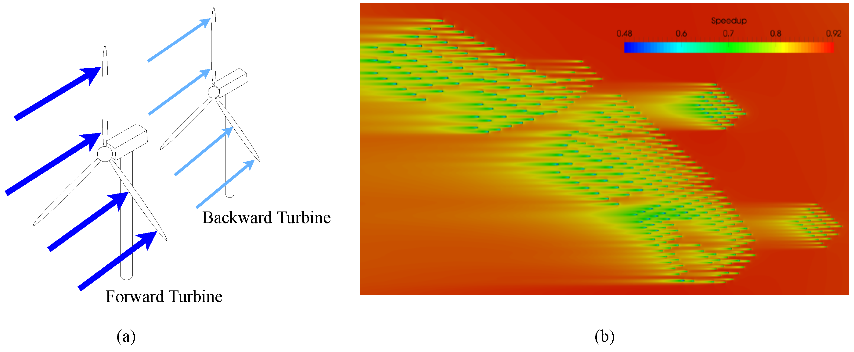
A wind farm is a power plant composed of arrays of WTs. The total power output of a wind farm is lower than the summation of power outputs of stand-alone WTs. This is because WTs at downstream locations produce less wind energy by encountering wake flow with less momentum due to the upstream turbines [41,42] (Figure 8a). The computational fluid dynamics (CFD) results in Figure 8b, which were generated with the framework developed in [43,44,45], provide an example of such wake effects for a wind farm. The velocity field of an offshore wind farm is shown with the easterly wind flowing from right to left. The wind farm is located in the North Sea and contains 370 neighboring WTs. It is clearly visible that the wind speed declines and that wake flow significantly affects wind power generation. Therefore, it is crucial to include wake effects when controlling all individual turbines in a wind farm.
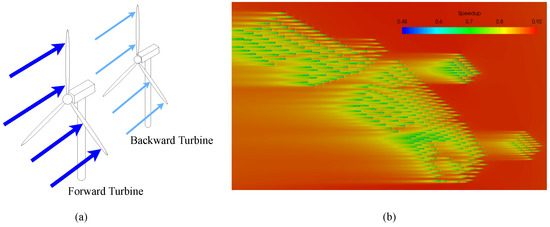
Figure 8.
(a) A schematic of the wake effect for two WTs. (b) CFD results showing wake effects in an offshore wind farm [45], reproduced with permission from Abel Gargallo-Peiró. Speedup stands for the velocity at each location divided by the upstream reference velocity.
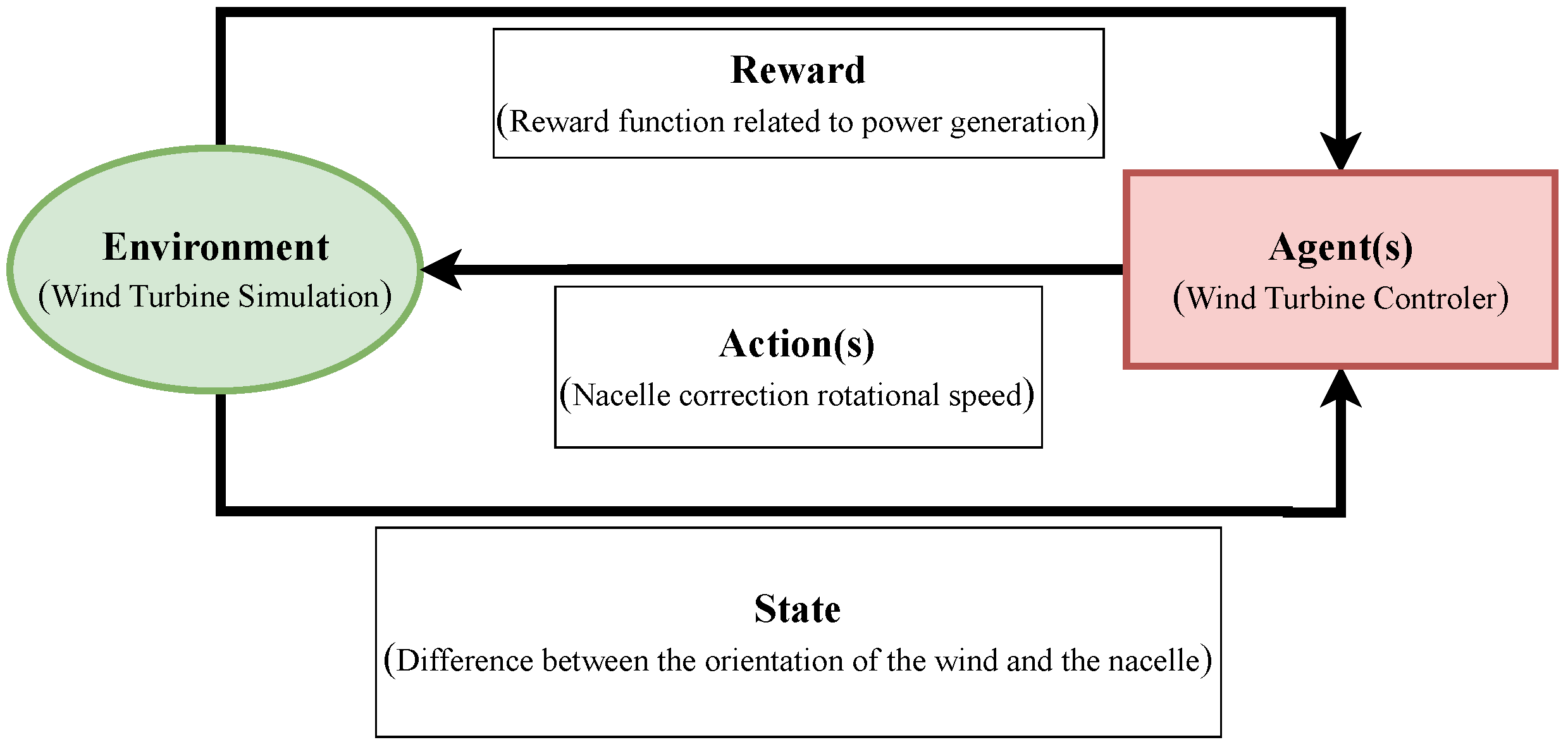
The most representative method to embed wake effects in yaw angle control systems is reinforcement learning (RL) [46,47,48]. RL is used to learn a sequence of actions that leads to an optimal state in an environment concerning a pre-defined optimization criterion. RL is an iterative mechanism where a single agent or multiple agents take an action based on a state provided by an environment. The environment then evaluates the action(s), provides feedback in the form of a reward, and passes the new state to the agent(s). A schematic diagram of controlling a wind farm using RL is shown in Figure 9. The optimum action(s) of changing the yaw angle of each WT based on a given state of wind flow could be learned with respect to the total power output. This can be achieved through trial and error explorations performed by an agent or agents, who are rewarded by a quantity related to energy production.
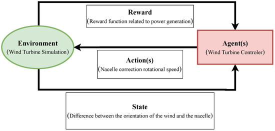
Figure 9.
Basic RL mechanism for wind farm control.
Zhao et al. [47] used an RL algorithm based on the deep deterministic policy gradient (DDPG) approach to control wind turbines in a wind farm. The DDPG is an RL algorithm for environments with continuous action space, such as yaw angles of WTs. For a discrete action space, each action could be evaluated with a so-called Q-value. For a continuous action space, however, the complete space cannot exhaustively be evaluated with this approach. Instead, a gradient-based learning rule is formulated that takes advantage of a Q-function that is differentiable with respect to the yaw angles chosen by an agent or multiple agents. For a more detailed explanation of DDPG, readers may refer to the following reference [49]. In [47], an algebraic wake model was used to model the wake effect and control the wind farm through knowledge-assisted learning DDPG (KA-DDPG). KA-DDPG constrains the learning of agents to physical rules and domain knowledge. Because of this constraint, an agent of KA-DDPG becomes capable of avoiding dangerous or low-reward actions. They reported improvement compared to a control algorithm (e.g., greedy algorithm) which does not involve any future consequences of an action of WTs. Similarly, Dong et al. [48] controlled WTs in a wind farm using a variant of DDPG. They reported a improvement in power production. It is also worth noting that they calculated the flow fields in a wind farm using high-fidelity simulations. Thus, no algebraic wake model was used.
Predicting the changes of flow fields due to wakes in wind farms using simulations is highly expensive, while algebraic wake models are inexpensive but inherently contain uncertainty. This is due to the challenging nature of accurately modeling turbulence and geometric effects. Therefore, developing an accurate wake model is important to improve the yaw control of wind farms. Recently, researchers have attempted to model wake by using NNs. For example, Li et al. [50] predicted unsteady turbine wakes using a CNN with two types of inputs. The first input is velocity field data over a certain time interval from the past. The second input is data of inflow velocity and yaw angle of each WT in the wind farm from the same past time interval. Their CNN model predicts the velocity fields at a future time based on these two inputs. The predictions under diverse conditions were compared with the result of large-eddy simulations (LES). LES computes turbulent flow by modeling sub-grid scale turbulence. Their CNN model showed an average error of 3.7% in predicting the wind velocity in a wind farm. Bleeg [51] developed a graphical neural network (GNN) to model wake effects. Reynolds-averaged Navier–Stokes (RANS) simulations were employed to generate training data. They developed a GNN that predicts the decay rate of wind speed in downstream locations relative to the front row of WTs. They reported that the developed GNN was capable of predicting the velocity decay rate with a small error (0.0028 in Mean absolute error). Table 2 summarizes the studies of yaw control and wind speed prediction in wind farms using NNs. The information on the employed machine learning method, the purpose of the study, the data source, and the quantitative performance of studies introduced in the current section are included in this table.

Table 2.
NN-based wind farm control and modeling methods.
4. NN-Based Turbine Blade Design
WTs convert the rotational energy of a rotor to a usable energy source. The rotation of rotors occurs due to the aerodynamic lift force generated on the turbine blade surfaces. The key to maximizing wind energy efficiency is to maximize the lift-to-drag ratio of a turbine blade. This ratio describes how effectively a blade can generate lift (i.e., rotation) while experiencing energy loss from drag. It is highly dependent on the shapes of the turbine blades and the flow conditions. Optimizing the design of a turbine blade aims to improve the lift-to-drag ratio at flow conditions in an operating WT. However, such an optimization process involves numerous design elements and conditions. In addition, for design robustness, flow analysis on the blade considering these factors should be repeated for various flow conditions. Therefore, the optimization process becomes costly. The increased computational costs can be overcome by employing NNs for efficiently designing optimal turbine blades.
Wen et al. [52] proposed a design method that combines a genetic algorithm and a back-propagation (GABP) NN to optimize the design of airfoils with reduced computational cost and complexity. Their NN was trained to predict a WT blade’s lift coefficient and lift-to-drag ratio, whose shape is represented by Bessel polynomials. The NN is reported to have a accuracy in predicting an arbitrary turbine blade’s lift coefficient and lift-to-drag ratio. Based on this network, the authors were able to design a blade with improved aerodynamic properties. Lalonde et al. [53] developed and compared six different NNs which function as surrogate models of an aerodynamic blade. These surrogate models are helpful because an NN connects input and output data without time-consuming computations such as CFD simulations. For example, they used the time-independent MLP with a full set of input data architecture with the following aerodynamic input data: wind speed, blade geometry, and blade deflected shape. Consequently, the CNN model predicted the aerodynamic load on the blade with a normalized root mean squared error (NRMSE) of 0.66%, where NRMSE is defined as:
where is the average of the ground truth values.
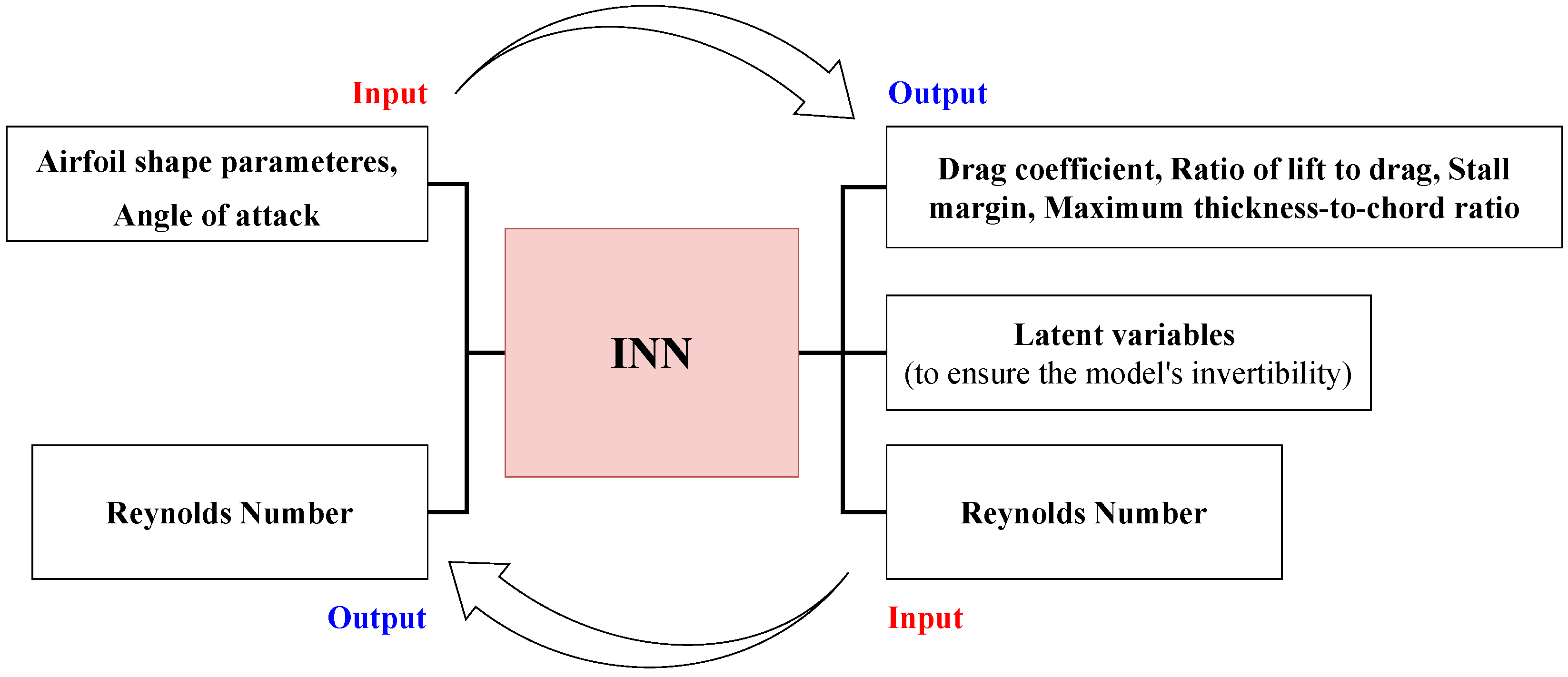
Jasa et al. [54] proposed an approach for an airfoil design that utilizes an invertible neural network (INN), as illustrated in Figure 10. An INN processes inputs to outputs and vice versa. The INN was trained with data acquired from two-dimensional numerical simulations of airfoils. The inputs of their INN are airfoil shapes and operating conditions, whereas the outputs are aerodynamic performances and structural considerations. The INN’s invertible nature allows the creation of an airfoil design that fully satisfies the desired aerodynamic performances and structural considerations. Their optimized blade is reported to increase the annual energy production by 3.4% compared to non-optimized airfoil.
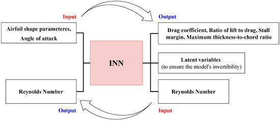
Figure 10.
Schematic of an INN architecture.
Oh [55] developed a neural network for predicting and optimizing the aerodynamic performances of WT airfoils. The developed NN demonstrated a superior optimization performance compared to conventional design methods, such as the response surface method (RSM) [56]. They found their NN suitable for learning the integrated influences of airfoil geometry and flow conditions on aerodynamic performances. Their optimized airfoil using NN showed 18.560% and 8.194% increases in the lift-to-drag ratio compared to an unoptimized airfoil and an airfoil optimized through RSM, respectively.
Jia et al. [57] demonstrated a tunable WT blade using RL. The twist angle distribution of the turbine blades was tuned using RL to maximize aerodynamic performances. Based on the power coefficient () of a blade with seven controllable actuators. they stated an average improvement of 12.9% in the high-speed wind regime (9∼13 m/s), but showed an average reduction in performance of -11.3% at low speed (5∼8 m/s), compared to blade control using a conventional genetic algorithm (GA). Table 3 summarizes the studies on designing WT blades using NNs. The information on the employed machine learning method, the purpose of the study, the data source, and the quantitative performance of studies introduced in the current section are included in this table.

Table 3.
NN-based turbine blade design methods.
5. Conclusions
WTs generate wind power from the kinetic energy of atmospheric flow. NNs are suitable for efficiently modeling the effects of atmospheric flow to wind power generation since NNs are capable of modeling non-linear functions. We investigated studies that have successfully improved power generation efficiency using NNs. To the best of our knowledge, we are the first to provide a review of neural-network-based methods to improve WT power generation in categories that cover wind turbines to wind farms and from control methods to blade design strategies.
First, studies focused on increasing the efficiency of a WT through the control of yaw angles were reviewed. In these studies, various types of NNs, e.g., MLP, LSTM, or CNN, were used to predict wind directions. Maximum power generation of a WT generally occurs when the nacelle direction and the wind direction are parallel. Based on accurate and fast wind predictions, the yaw of a WT can be controlled to achieve an optimal position and increase power generation.
Second, studies aimed at improving the energy efficiency of wind farms were reviewed. Due to the momentum loss at upstream WTs’ wake, the total power generation of a wind farm is inevitably lower than the sum of the maximum power generation of individual WTs. Typically, quantifying such interactions, e.g., wake flows, is computationally expensive. This renders the analysis of a wind farm arrangement difficult. We reviewed studies that employ NNs to overcome this limitation. A number of studies employed RL to control wind farms in a way that minimizes the negative effects of interactions between WTs and maximizes total power output. Other studies concentrate on modeling complex wake effects by developing NN-based surrogate models.
Finally, NN- and RL-based studies that optimized WT blade designs to improve the aerodynamic performances of WTs were reviewed. An optimization of turbine blades normally requires iterative CFD computations. Since CFD is a time-consuming method that requires a large amount of computational resources, NN-based surrogate models of CFD have been actively proposed. The developed surrogate models show a small margin of error and only take a fraction of the time needed to conduct simulations, leading to blade designs with improved wind power generation efficiency.
Author Contributions
Conceptualization, H.S. and S.L.; formal analysis, H.S. and M.R.; investigation, H.S. and M.R.; writing—original draft preparation, H.S.; writing—review and editing, M.R. and S.L.; visualization, H.S.; supervision, S.L.; project administration, S.L.; funding acquisition, S.L. All authors have read and agreed to the published version of the manuscript.
Funding
This research was supported by INHA UNIVERSITY Research Grant (2022).
Institutional Review Board Statement
Not applicable.
Informed Consent Statement
Not applicable.
Data Availability Statement
Not applicable.
Acknowledgments
This work was performed as part of the Helmholtz School for Data Science in Life, Earth, and Energy (HDS-LEE).
Conflicts of Interest
The authors declare no conflict of interest.
Abbreviations
The following abbreviations are used in this manuscript:
| WT | Wind Turbine |
| ML | Machine Learning |
| NN | Neural Network |
| HAWT | Horizontal-Axis Wind Turbine |
| VAWT | Vertical-Axis Wind Turbine |
| UWT | Upwind Wind Turbine |
| DWT | Downwind Wind Turbine |
| PID | Proportional–Integral–Derivative |
| PI | Proportional–Integral |
| MLP | Multi-Layer Perceptron |
| ReLU | Rectified Linear Unit |
| RNN | Recurrent Neural Network |
| LSTM | Long Short-Term Memory |
| CNN | Convolutional Neural Network |
| LES | Large Eddy Simulation |
| RL | Reinforcement Learning |
| CFD | Computational Fluid Dynamics |
| RANS | Reynolds Averaged Numerical Simulation |
| MSE | Mean Square Error |
| NMSE | Normalized Mean Square Error |
| MAPE | Mean Absolute Percentage Error |
| DDPG | Deep Deterministic Policy Gradient |
| GABP | Genetic Algorithms Back Propagation |
| RMSE | Root Mean Squared Error |
| NRMSE | Normalized Root Mean Squared Error |
| RSM | Response Surface Method |
| INN | Invertible Neural Network |
| GA | Genetic Algorithm |
| GNN | Graph Neural Network |
Appendix A. Wind Turbines
WTs can be categorized into horizontal-axis wind turbines (HAWT) and vertical-axis wind turbines (VAWT). This classification is determined by the direction of the axis of rotation of the blade. The axis of rotation of the HAWT is horizontal to the wind. The advantage of a HAWT is that it has a higher power generation efficiency than a VAWT [58,59]. However, HAWTs must change the nacelle direction to maintain maximum power generation. In addition, a sufficiently large space must be secured when constructing a wind farm because aerodynamic interference occurs between adjacent turbines due to wake formation [60,61]. In contrast, the axis of rotation of a VAWT is perpendicular to the wind direction. VAWTs take in wind from all directions. Therefore, they do not require a yaw system, and most of the mechanical parts are located in the ground. Consequently, VAWTs bear simpler structures, and their maintenance is easier than HAWTs. In addition, a VAWT wind farm can be constructed more densely than a wind farm composed of HAWTs [59,61,62]. Despite the advantages of a VAWT, it is rarely used because of its lower power generation efficiency than HAWT. [58,59]. Therefore, only HAWT is considered in the current study.
HAWTs can be further categorized into two sub-classes, based on the direction of the nacelle: (i) an upwind wind turbine (UWT) where the nacelle direction is opposite to the wind, and (ii) a downwind wind turbine (DWT) where the nacelle direction is aligned to the wind (Figure A1). Unlike a DWT, a UWT does not have a tower shadow effect where the generator pillar causes periodic changes in the wind flow. The tower shadow effect negatively affects the lifespan of the blades due to increased fatigue [63]. Therefore UWTs are used more frequently than DWTs.
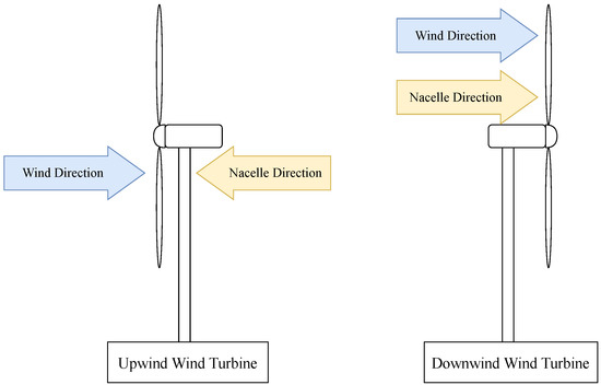
Figure A1.
Schematic diagrams of a UWT and DWT.
Figure A1.
Schematic diagrams of a UWT and DWT.
References
- Suresh, K. Climate Change Challenge 26 th Conference of Parties (COP26) climate summit is crucial but may be disappointing? Glob. J. Ecol. 2021, 6, 100–104. [Google Scholar]
- Joyce Lee, F.Z. Global Wind Report 2022; Technical Report; Global Wind Energy Council: Brussels, Belgium, 2022. [Google Scholar]
- Weschenfelder, F.; Leite, G.d.N.P.; da Costa, A.C.A.; de Castro Vilela, O.; Ribeiro, C.M.; Ochoa, A.A.V.; Araujo, A.M. A review on the complementarity between grid-connected solar and wind power systems. J. Clean. Prod. 2020, 257, 120617. [Google Scholar] [CrossRef]
- Njiri, J.G.; Söffker, D. State-of-the-art in wind turbine control: Trends and challenges. Renew. Sustain. Energy Rev. 2016, 60, 377–393. [Google Scholar] [CrossRef]
- More, A.; Deo, M. Forecasting wind with neural networks. Mar. Struct. 2003, 16, 35–49. [Google Scholar] [CrossRef]
- Jie, W.; Jingchun, C.; Lin, Y.; Wenliang, W.; Jian, D. Pitch control of wind turbine based on deep neural network. IOP Conf. Ser. Earth Environ. Sci. 2020, 619, 012034. [Google Scholar]
- Wang, Y.; Zou, R.; Liu, F.; Zhang, L.; Liu, Q. A review of wind speed and wind power forecasting with deep neural networks. Appl. Energy 2021, 304, 117766. [Google Scholar] [CrossRef]
- Lin, Z.; Liu, X. Wind power forecasting of an offshore wind turbine based on high-frequency SCADA data and deep learning neural network. Energy 2020, 201, 117693. [Google Scholar] [CrossRef]
- Leite, G.d.N.P.; da Cunha, G.T.M.; dos Santos Junior, J.G.; Araújo, A.M.; Rosas, P.A.C.; Stosic, T.; Stosic, B.; Rosso, O.A. Alternative fault detection and diagnostic using information theory quantifiers based on vibration time-waveforms from condition monitoring systems: Application to operational wind turbines. Renew. Energy 2021, 164, 1183–1194. [Google Scholar] [CrossRef]
- Correa-Jullian, C.; Cofre-Martel, S.; San Martin, G.; Lopez Droguett, E.; de Novaes Pires Leite, G.; Costa, A. Exploring Quantum Machine Learning and Feature Reduction Techniques for Wind Turbine Pitch Fault Detection. Energies 2022, 15, 2792. [Google Scholar] [CrossRef]
- Schlechtingen, M.; Santos, I.F. Comparative analysis of neural network and regression based condition monitoring approaches for wind turbine fault detection. Mech. Syst. Signal Process. 2011, 25, 1849–1875. [Google Scholar] [CrossRef]
- Menezes, E.J.N.; Araújo, A.M.; Da Silva, N.S.B. A review on wind turbine control and its associated methods. J. Clean. Prod. 2018, 174, 945–953. [Google Scholar] [CrossRef]
- Gao, R.; Gao, Z. Pitch control for wind turbine systems using optimization, estimation and compensation. Renew. Energy 2016, 91, 501–515. [Google Scholar] [CrossRef]
- Yin, X.X.; Lin, Y.G.; Li, W.; Gu, Y.J. Integrated pitch control for wind turbine based on a novel pitch control system. J. Renew. Sustain. Energy 2014, 6, 043106. [Google Scholar] [CrossRef]
- Selvam, K.; Kanev, S.; van Wingerden, J.W.; van Engelen, T.; Verhaegen, M. Feedback–feedforward individual pitch control for wind turbine load reduction. Int. J. Robust Nonlinear Control. IFAC-Affil. J. 2009, 19, 72–91. [Google Scholar] [CrossRef]
- Sierra-Garcia, J.E.; Santos, M. Deep learning and fuzzy logic to implement a hybrid wind turbine pitch control. Neural Comput. Appl. 2022, 34, 10503–10517. [Google Scholar] [CrossRef]
- Hure, N.; Turnar, R.; Vašak, M.; Benčić, G. Optimal wind turbine yaw control supported with very short-term wind predictions. In Proceedings of the 2015 IEEE International Conference on Industrial Technology (ICIT), Seville, Spain, 17–19 March 2015; IEEE: Piscataway, NJ, USA, 2015; pp. 385–391. [Google Scholar]
- Chen, W.; Liu, H.; Lin, Y.; Li, W.; Sun, Y.; Zhang, D. LSTM-NN yaw control of wind turbines based on upstream wind information. Energies 2020, 13, 1482. [Google Scholar] [CrossRef]
- Kim, M.; Dalhoff, P. Yaw Systems for wind turbines–Overview of concepts, current challenges and design methods. J. Phys. Conf. Ser. 2014, 524, 012086. [Google Scholar]
- Yang, J.; Fang, L.; Song, D.; Su, M.; Yang, X.; Huang, L.; Joo, Y.H. Review of control strategy of large horizontal-axis wind turbines yaw system. Wind Energy 2021, 24, 97–115. [Google Scholar] [CrossRef]
- Kani, S.P.; Ardehali, M. Very short-term wind speed prediction: A new artificial neural network–Markov chain model. Energy Convers. Manag. 2011, 52, 738–745. [Google Scholar] [CrossRef]
- Ðalto, M.; Vašak, M.; Baotic, M.; Matuško, J.; Horvath, K. Neural-network-based ultra-short-term wind forecasting. In Proceedings of the European Wind Energy Association 2014 Annual Event (EWEA 2014), Barcelona, Spain, 10–13 March 2014. [Google Scholar]
- Molano, D.E.A.; Vargas, D.A.B. Wind Turbine Yaw Angle Control using Artificial Neural Networks: Real data is used to feed the neural network. In Proceedings of the 2020 10th International Conference on Advanced Computer Information Technologies (ACIT), Deggendorf, Germany, 16–18 September 2020; IEEE: Piscataway, NJ, USA, 2020; pp. 374–379. [Google Scholar]
- Dzulfikri, Z.; Nuryanti, N.; Erdani, Y. Design and implementation of artificial neural networks to predict wind directions on controlling yaw of wind turbine prototype. J. Robot. Control. (JRC) 2020, 1, 20–26. [Google Scholar] [CrossRef]
- Zhang, L.; He, S.; Cheng, J.; Yuan, Z.; Yan, X. Research on neural network wind speed prediction model based on improved sparrow algorithm optimization. Energy Rep. 2022, 8, 739–747. [Google Scholar] [CrossRef]
- Sharma, S.; Sharma, S.; Athaiya, A. Activation functions in neural networks. Towards Data Sci. 2017, 6, 310–316. [Google Scholar] [CrossRef]
- Krizhevsky, A.; Sutskever, I.; Hinton, G.E. Imagenet classification with deep convolutional neural networks. Commun. ACM 2017, 60, 84–90. [Google Scholar] [CrossRef]
- Maas, A.L.; Hannun, A.Y.; Ng, A.Y. Rectifier nonlinearities improve neural network acoustic models. In Proceedings of the Proceeding ICML, Atlanta, GA, USA, 16–21 June 2013; Volume 30, p. 3. [Google Scholar]
- Xu, B.; Wang, N.; Chen, T.; Li, M. Empirical evaluation of rectified activations in convolutional network. arXiv 2015, arXiv:1505.00853. [Google Scholar]
- Delgado, I.; Fahim, M. Wind turbine data analysis and LSTM-based prediction in SCADA system. Energies 2020, 14, 125. [Google Scholar] [CrossRef]
- Zhang, J.; Jiang, X.; Chen, X.; Li, X.; Guo, D.; Cui, L. Wind power generation prediction based on LSTM. In Proceedings of the 2019 4th International Conference on Mathematics and Artificial Intelligence, Chengdu, China, 12–15 April 2019; pp. 85–89. [Google Scholar]
- Lee, S.; You, D. Data-driven prediction of unsteady flow over a circular cylinder using deep learning. J. Fluid Mech. 2019, 879, 217–254. [Google Scholar] [CrossRef]
- Rüttgers, M.; Lee, S.; Jeon, S.; You, D. Prediction of a typhoon track using a generative adversarial network and satellite images. Sci. Rep. 2019, 9, 1–15. [Google Scholar] [CrossRef]
- Fukami, K.; Fukagata, K.; Taira, K. Machine-learning-based spatio-temporal super resolution reconstruction of turbulent flows. J. Fluid Mech. 2021, 909, A9. [Google Scholar] [CrossRef]
- Kim, J.; Lee, C. Prediction of turbulent heat transfer using convolutional neural networks. J. Fluid Mech. 2020, 882, A18. [Google Scholar] [CrossRef]
- Harbola, S.; Coors, V. One dimensional convolutional neural network architectures for wind prediction. Energy Convers. Manag. 2019, 195, 70–75. [Google Scholar] [CrossRef]
- Hong, Y.Y.; Satriani, T.R.A. Day-ahead spatiotemporal wind speed forecasting using robust design-based deep learning neural network. Energy 2020, 209, 118441. [Google Scholar] [CrossRef]
- Wu, Q.; Zheng, H.; Guo, X.; Liu, G. Promoting wind energy for sustainable development by precise wind speed prediction based on graph neural networks. Renew. Energy 2022, 199, 977–992. [Google Scholar] [CrossRef]
- Scarselli, F.; Gori, M.; Tsoi, A.C.; Hagenbuchner, M.; Monfardini, G. The graph neural network model. IEEE Trans. Neural Netw. 2008, 20, 61–80. [Google Scholar] [CrossRef]
- Vaswani, A.; Shazeer, N.; Parmar, N.; Uszkoreit, J.; Jones, L.; Gomez, A.N.; Kaiser, Ł.; Polosukhin, I. Attention is all you need. In Proceedings of the 31st International Conference on Neural Information Processing Systems, Long Beach, CA, USA, 4–9 December 2017. [Google Scholar]
- Choi, N.J.; Nam, S.H.; Jeong, J.H.; Kim, K.C. Numerical study on the horizontal axis turbines arrangement in a wind farm: Effect of separation distance on the turbine aerodynamic power output. J. Wind. Eng. Ind. Aerodyn. 2013, 117, 11–17. [Google Scholar] [CrossRef]
- González-Longatt, F.; Wall, P.; Terzija, V. Wake effect in wind farm performance: Steady-state and dynamic behavior. Renew. Energy 2012, 39, 329–338. [Google Scholar] [CrossRef]
- Avila, M.; Gargallo-Peiró, A.; Folch, A. A CFD framework for offshore and onshore wind farm simulation. J. Phys. Conf. Ser. 2017, 854, 012002. [Google Scholar]
- Gargallo-Peiró, A.; Avila, M.; Owen, H.; Prieto, L.; Folch, A. Mesh Generation for Atmospheric Boundary Layer Simulation in Wind Farm Design and Management. Procedia Eng. 2015, 124, 239–251. [Google Scholar] [CrossRef]
- Gargallo-Peiró, A.; Avila, M.; Owen, H.; Prieto-Godino, L.; Folch, A. Mesh generation, sizing and convergence for onshore and offshore wind farm Atmospheric Boundary Layer flow simulation with actuator discs. J. Comput. Phys. 2018, 375, 209–227. [Google Scholar] [CrossRef]
- Saenz-Aguirre, A.; Zulueta, E.; Fernandez-Gamiz, U.; Lozano, J.; Lopez-Guede, J.M. Artificial neural network based reinforcement learning for wind turbine yaw control. Energies 2019, 12, 436. [Google Scholar] [CrossRef]
- Zhao, H.; Zhao, J.; Qiu, J.; Liang, G.; Dong, Z.Y. Cooperative Wind Farm Control With Deep Reinforcement Learning and Knowledge-Assisted Learning. IEEE Trans. Ind. Inform. 2020, 16, 6912–6921. [Google Scholar] [CrossRef]
- Dong, H.; Zhang, J.; Zhao, X. Intelligent wind farm control via deep reinforcement learning and high-fidelity simulations. Appl. Energy 2021, 292, 116928. [Google Scholar] [CrossRef]
- Lillicrap, T.P.; Hunt, J.J.; Pritzel, A.; Heess, N.; Erez, T.; Tassa, Y.; Silver, D.; Wierstra, D. Continuous control with deep reinforcement learning. arXiv 2015, arXiv:1509.02971. [Google Scholar]
- Li, R.; Zhang, J.; Zhao, X. Dynamic wind farm wake modeling based on a Bilateral Convolutional Neural Network and high-fidelity LES data. Energy 2022, 258, 124845. [Google Scholar] [CrossRef]
- Bleeg, J. A graph neural network surrogate model for the prediction of turbine interaction loss. J. Phys. Conf. Ser. 2020, 1618, 062054. [Google Scholar]
- Wen, H.; Sang, S.; Qiu, C.; Du, X.; Zhu, X.; Shi, Q. A new optimization method of wind turbine airfoil performance based on Bessel equation and GABP artificial neural network. Energy 2019, 187, 116106. [Google Scholar] [CrossRef]
- Lalonde, E.; Vischschraper, B.; Bitsuamlak, G.; Dai, K. Evaluation of a neural network-based surrogate aerodynamic wind turbine model. In Proceedings of the International Conference on Advances in Wind and Structures, Seoul, Republic of Korea, 25–29 August 2020; Volume 8. [Google Scholar]
- Jasa, J.; Glaws, A.; Bortolotti, P.; Vijayakumar, G.; Barter, G. Wind turbine blade design with airfoil shape control using invertible neural networks. J. Phys. Conf. Ser. 2022, 2265, 042052. [Google Scholar]
- Oh, S. Comparison of a response surface method and artificial neural network in predicting the aerodynamic performance of a wind turbine airfoil and its optimization. Appl. Sci. 2020, 10, 6277. [Google Scholar] [CrossRef]
- Allaix, D.L.; Carbone, V.I. An improvement of the response surface method. Struct. Saf. 2011, 33, 165–172. [Google Scholar] [CrossRef]
- Jia, L.; Hao, J.; Hall, J.; Nejadkhaki, H.K.; Wang, G.; Yan, Y.; Sun, M. A reinforcement learning based blade twist angle distribution searching method for optimizing wind turbine energy power. Energy 2021, 215, 119148. [Google Scholar] [CrossRef]
- Saad, M.M.M.; Asmuin, N. Comparison of horizontal axis wind turbines and vertical axis wind turbines. IOSR J. Eng. (IOSRJEN) 2014, 4, 27–30. [Google Scholar] [CrossRef]
- Cheng, K.; Wang, Z.; He, Y.; Yang, G. The comparison of theoretical potential application of two types of wind turbines in Northern Shaanxi. In Proceedings of the 2012 Asia-Pacific Power and Energy Engineering Conference, Shanghai, China, 27–29 March 2012; IEEE: Piscataway, NJ, USA, 2012; pp. 1–4. [Google Scholar]
- Tjiu, W.; Marnoto, T.; Mat, S.; Ruslan, M.H.; Sopian, K. Darrieus vertical axis wind turbine for power generation II: Challenges in HAWT and the opportunity of multi-megawatt Darrieus VAWT development. Renew. Energy 2015, 75, 560–571. [Google Scholar] [CrossRef]
- Dabiri, J. Potential order-of-magnitude enhancement of wind farm power density via counter-rotating vertical-axis wind turbine arrays. J. Renew. Sustain. Energy 2011, 3, 043104. [Google Scholar] [CrossRef]
- Paraschivoiu, I. Wind Turbine Design: With Emphasis on Darrieus Concept; Presses inter Polytechnique: Montréal, QC, Canada, 2002. [Google Scholar]
- Powles, S. The effects of tower shadow on the dynamics of a horizontal-axis wind turbine. Wind Eng. 1983, 7, 26–42. [Google Scholar]
Publisher’s Note: MDPI stays neutral with regard to jurisdictional claims in published maps and institutional affiliations. |
© 2022 by the authors. Licensee MDPI, Basel, Switzerland. This article is an open access article distributed under the terms and conditions of the Creative Commons Attribution (CC BY) license (https://creativecommons.org/licenses/by/4.0/).

