A Novel BEM–FEM Scheme for the Interaction of Water Waves with Multiple Vertical Cylinders in the Presence of Currents

Abstract

The interaction of waves and currents with marine structures finds interesting applications, including the study of offshore and shoreline protection systems, as in the case of permeable breakwaters. The latter systems exhibit various benefits, including a decrease in wave run-up, reflected wave energy and load excitation, allowing for the propagation of part of the incident flow to the lee side, facilitating the improvement of water quality in the protected areas. The present work focuses on the modelling and numerical simulation of wave fields, interacting with arrays of vertical cylinders in the presence of currents. The problem is treated in the framework of potential theory in the frequency domain, assuming waves of small steepness, in conjunction with boundary integral formulation. Numerical results are presented and discussed, concerning the structure of the reflected and transmitted 3D flow fields, making the model suitable for optimization purposes; however, it presents increased computational cost. On the other hand, for small current velocities the problem can be approximately considered on the horizontal plane, modelled by the 2D Helmholtz equation with variable coefficients, which is numerically treated by a coupled BEM–FEM scheme. Numerical examples are presented, demonstrating that the latter model is cost-efficient, providing reasonable predictions, and can be used for the preliminary study of the hydrodynamic characteristics of the considered configurations and the support of the design.

1. Introduction

Knowledge of the properties of water waves in nearshore regions is essential for the design and optimization of coastal defense systems. The latter is a subject of particular interest especially in coastal engineering, aiming towards the conservation and protection of inhabited areas, as well as other areas of interest, from loads arising due to interaction with the highly dynamic marine environment. Permeable breakwaters, see, e.g., [1], are a case exhibiting various benefits, including a decrease in wave run-up, reflected wave energy and load excitation, allowing for the propagation of part of the incident flow to the lee side, facilitating the improvement of water quality in protected areas. Among several protection systems concerning permeable breakwaters, one particular class consists of arrays of vertical cylinders, as presented in Figure 1. The problem of wave propagation through such structures has been addressed by several researchers, providing useful data by both experimental (e.g., Arnaud et al. [2]) and numerical studies (Belibassakis et al. [3,4]) concerning wave reflection and dissipation. Similar structures have been studied as sloshing dampers in tanks by Molin et al. [5]; see also Jamain et al. [6].

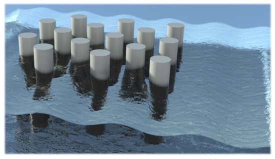
Figure 1. Configuration of the arrangement of vertical cylinders considered as permeable breakwaters.

Moreover, wave diffraction by arrays of vertical circular cylinders in a channel is an interesting subject concerning the study of strong Bragg resonances, see, e.g., Li and Mei [7], as well as the investigation of appearance of trapped modes; see, e.g., Linton and McIver [8] and Utsunomiya and Eatock Taylor [9], and the references cited therein. The above problems find useful applications in the analysis of large structures, such as offshore airports supported on vertical piles, and the design of marine renewable energy systems.

Furthermore, the effects of currents on water wave propagation and interaction with the seabed and structures often prove to be significant, since they result in Doppler effects causing additional refraction, reflection, and breaking phenomena. The above may radically change the pattern of energy propagation in a fluid channel with obstructions (see, e.g., [3]). The prediction of loads on cylindrical structures arising due to wave–current interaction (Sumer and Fredsoe [10]) is becoming increasingly important as the number of bottom-founded and floating marine structures grows, driven, among other factors, by the development of ocean energy plants. This fact has been also demonstrated by recent works focusing on the experimental study of wave–current interaction effects on the wave loads on vertical surface piercing cylinder; see, e.g., Ghadirian et al. [11].

The wave-current-body hydrodynamic interaction problems are usually examined in the context of potential flow applications, and the consideration of harmonic waves (see, e.g., Thomas [12]) facilitates the preliminary analysis and investigation of the field features, and supports the engineering studies concerning the loads on structures. The present work focuses on the modelling and numerical simulation of wave fields interacting with arrangements of vertical cylinders within a waveguide, in the presence of currents. The configuration is considered to consist of arrays of bottom-seated vertical cylinders, extending all over the water column; see Figure 1. For relatively slow currents, the problem is decomposed into steady and wave flow parts and is treated by 3D BEM. Numerical results are presented and discussed, concerning the structure of the reflected and transmitted flow fields, making the model suitable for optimization purposes. However, the 3D model presents increased computational cost. For this reason, the problem is approximately reformulated and treated on the horizontal plane, modelled by the 2D Helmholtz equation with variable coefficient. The above approximate reformulation of the problem for small current velocity is a novelty of the present work, and substantially reduces the computational cost. In particular, for the latter simplified formulation, a coupled BEM–FEM scheme is proposed for the numerical simulation of wave fields propagating over multiple vertical cylinder arrays, in the presence of currents. Numerical examples are presented and compared with the 3D BEM for verification, including data concerning the memory and time requirements, demonstrating that the above model is cost-efficient, provides reasonable predictions and can be used for the preliminary study of the hydrodynamic characteristics of the considered configurations and support design.

2. Mathematical Formulation of the 3D Problem

Let $D\in {ℝ}^3$ denote the constant depth water domain including the vertical cylinders. A Cartesian coordinate system $x=\left(x_1,x_2,x_3\right)$ is introduced, with the origin placed on Still Water Level (SWL), with the $x_3$-axis pointing upwards, as illustrated in Figure 2. The domain $D$ is bounded by the free surface of the water $\left(\partial D_{FS}\right)$ and the impenetrable bottom $\left(\partial D_B\right)$ located at $x_3=-h$, where $h$ is the constant water depth. Finally, the wetted surfaces of all cylinders are denoted by $\partial D_{\hspace{0.17em}WS}$. Based on standard linear water-wave theory, the velocity field in $D$ is expressed by the gradient of the (scalar) potential function $\Phi$ which satisfies the Laplace equation in the domain.

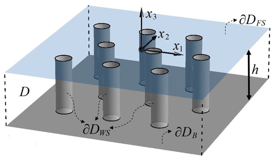
Figure 2. Coordinate system and geometrical configuration of the 3D problem.

In cases of waves propagating under the additional effects of slow steady currents, the flow variables can be decomposed into a steady background current field and the time-dependent wave part which, in the present work, is considered as harmonic. The latter components are described by the potential functions of the incident (I) and the perturbation–diffraction (D) fields, for both the steady ${\phi }^{(S)}(x)$ and the unsteady ${\phi }^{(U)}(x;\hspace{0.17em}t)$ potential functions. Let U denote the steady current field velocity on and near the free surface. Following the standard formulation, the free surface boundary conditions for the wave field are linearized as follows (see, e.g., Belibassakis et al. [3,13]):

$$\frac{D\eta \left(x\right)}{Dt}-\frac{\partial \phi \left(x\right)}{\partial x_3}=0,\hspace{0.17em}\hspace{0.17em}\hspace{0.17em}x\in \partial D_{FS},$$

(1a)

$$\frac{D\phi \left(x\right)}{Dt}+g\eta \left(x\right)=0,\hspace{0.17em}\hspace{0.17em}\hspace{0.17em}x\in \partial D_{FS},$$

(1b)

where $D/Dt=\partial /\partial t+U{\nabla }_h$, with ${\nabla }_h$ denoting the horizontal gradient ${\nabla }_h=\left(\partial /\partial x_1,\partial /\partial x_2\right)$, $\eta \left(x\right)$ being the free surface elevation and $\phi$ the corresponding wave potential. By eliminating $\eta \left(x\right)$ from Equations (1a) and (1b) and using Equation (1a), we obtain:

$$\frac{D^2\phi \left(x\right)}{D{t}^2}+g\frac{\partial \phi \left(x\right)}{\partial x_3}=0,\hspace{0.17em}\hspace{0.17em}\hspace{0.17em}x\in \partial D_{FS}.$$

(2)

In the present work, the wave field is excited by monochromatic incident waves, allowing us to consider harmonic time dependence as follows:

$${\Phi }^{(U)}\left(x;\hspace{0.17em}t\right)=\mathrm{Re}\left\{{\phi }^{(U)}\left(x\right)\cdot \exp \left(-i\hspace{0.17em}\omega \hspace{0.17em}t\right)\right\},$$

(3)

where $\omega$ is the absolute frequency of the incident wave field, which also coincides with the angular frequency of the diffracted unsteady field, due to linearity of the governing equation, and $i=\sqrt{-1}$. Using the representation ${\phi }^{(U)}\left(x\right)=F\left(x\right)\exp \left(iS\left(x\right)\right)$, where $F\left(x\right),\hspace{0.17em}\hspace{0.17em}S\left(x\right)$ are the modulus and the phase of the complex wave potential, respectively, and assuming slow current and mild variation of the field modulus, from the above equations we obtain:

$$\frac{\partial {\phi }^{(U)}\left(x\right)}{\partial x_3}+\frac{{\sigma }^2}{g}{\phi }^{(U)}\left(x\right)=0,\hspace{1em}x\in \partial D_{FS},$$

(4)

where $\sigma =\omega -U{\nabla }_{h}S=\omega -kU$ denotes the intrinsic frequency and $k={\nabla }_{h}S$ denotes the generally spatially variable wavenumber vector on the free surface.

Following the standard decomposition approach used for wave interaction problems in ship and marine hydrodynamics, the surface flow $U$ is calculated from the solution of a steady flow problem $\left({\phi }^{(S)}(x)\right)$, which satisfies the Laplace equation and the no-entrance boundary condition on the vertical cylinders and the impermeable seabed. Thus, the total flow field is represented by the following superposition:

$$\Phi \left(x;\hspace{0.17em}t\right)={\phi }^{(S)}(x)+\mathrm{Re}\left\{{\phi }^{(U)}\left(x\right)\cdot \exp \left(-i\hspace{0.17em}\omega \hspace{0.17em}t\right)\right\}.$$

(5)

The complex wave potential is further decomposed into incident wave ${\phi }_I^{(U)}\left(x\right)$ and diffraction ${\phi }_D^{(U)}\left(x\right)$ components, i.e., ${\phi }^{(U)}\left(x\right)={\phi }_I^{(U)}\left(x\right)+{\phi }_D^{(U)}\left(x\right)$. The former part is associated with the incident wave that is defined in the absence of the disturbance generated by the scatterers, which is described by the diffraction component. For simplicity, we consider here that the steady flow upstream behaves as a parallel incident flow directed downstream along the x₁-axis; thus, in the far upstream region, ${\phi }_I^{(S)}(x)\approx -U_{\infty }{x}_{\hspace{0.17em}1}$, with $U_{\infty }$ being the current velocity far from the cylinders. Based on the above, the incident wave potential is defined as:

$${\phi }_I^{(U)}\left(x\right)=-\frac{igH}{2{\sigma }_I}\frac{\cosh \left(k_I\left(x_{\hspace{0.17em}3}+h\right)\right)}{\cosh \left(k_{I}h\right)}\exp \left(-i{k}_I{x}_1\right),$$

(6)

where H is the wave height, ${\sigma }_I=\omega -k_I{U}_{\infty }$, and the incident wavenumber $k_{\hspace{0.17em}I}$ is obtained by the dispersion relation:

$${\sigma }_I^2\equiv {\left(\omega -k_I{U}_{\infty }\right)}^2=k_{I}g\tanh \left(k_{I}h\right).$$

(7)

In this work, the current and waves are assumed to be collinear directed along the x₁-axis; however, generalization of the incident flow directed at an angle is possible. The above considerations allow for the formulation of the problems for the steady ${\phi }_D^{(S)}(x)$ and the unsteady ${\phi }_D^{(U)}\left(x\right)$ diffraction fields in the domain and the development of suitable 3D Boundary Element Methods for their solution, as described in the following sections.

2.1. Formulation of the 3D Steady Current Flow Problem

As stated above, the steady background current is defined by the interaction of a uniform parallel flow $U_{\infty }=\left(-U_{\infty },0,0\right)$ directed towards the negative $x_1$-axis, with the cylinders in the constant depth strip. Thus, in the upstream region, the steady flow behaves as:

$${\phi }^{(S)}(x)\approx {\phi }_I^{(S)}(x)\equiv -U_{\infty }{x}_{\hspace{0.17em}1},\hspace{1em}{x}_{\hspace{0.17em}1}\to \infty .$$

(8)

The perturbation field is calculated following a Neumann–Kelvin (NK) formulation (see, e.g., Noblesse [14]) using the decomposition:

$${\phi }^{(S)}(x)={\phi }_I^{(S)}(x)+{\phi }_D^{(S)}(x).$$

(9)

The steady perturbation field ${\phi }_D^{(S)}(x)$, which is expected to present wavelike behavior downstream the cylinders, is calculated as a solution to the Laplace equation, subjected to the free-surface boundary condition and the no-entrance conditions at the seabed and the wetted surface of the bodies:

$${\nabla }^2{\phi }_D^{(S)}\left(x\right)=0,\hspace{0.17em}\hspace{0.17em}x\in D,\hspace{0.17em}$$

(10a)

$$\frac{{\partial }^2{\phi }_D^{(S)}\left(x\right)}{\partial x_1^2}+\frac{g}{U_{\infty }^2}\frac{\partial {\phi }_D^{(S)}\left(x\right)}{\partial x_3}=0,\hspace{0.17em}x\in \partial D_{FS},$$

(10b)

$$\frac{\partial {\phi }_D^{(S)}\left(x\right)}{\partial n}=-U_{\infty }\hspace{0.17em}n=U_{\infty }\hspace{0.17em}{n}_1,\hspace{0.17em}\hspace{0.17em}x\in \partial D_{WS},$$

(10c)

$$\frac{\partial {\phi }_D^{(S)}\left(x\right)}{\partial n}=0,\hspace{0.17em}\hspace{0.17em}x\in \partial D_B,$$

(10d)

as well as appropriate conditions at infinity. In Equation (10a)–(10d), $n=\left(n_1,n_2,n_3\right)$ denotes the unit vector, normal to the boundary $\partial D$, directed towards the exterior of $D$. The problem is treated by means of a panel method using simple singularity distributions; see, e.g., Katz and Plotkin [15]. The following integral representation is introduced for the potential function ${\phi }_D^{(S)}\left(x\right)$ in the domain $D$:

$${\phi }_D^{(S)}\left(x\right)={\displaystyle \underset{\partial D}{\int }{\mu }^{(S)}\left(x^{\prime }\right)G\left(x^{\prime },x\right)dS\left(x^{\prime }\right)},\hspace{0.17em}\hspace{0.17em}x\in D,\hspace{0.17em}\hspace{0.17em}{x}^{\prime }\in \partial \widehat{D},$$

(11a)

where $\partial \widehat{D}=\partial D_{FS}\cup \partial D_{WS}$ is the total boundary of the flow field, excluding the seabed $\left(\partial D_B\right)$, and

$$G\left(x^{\prime },x\right)=\frac{1}{4\pi }\left(\frac{1}{\left|x^{\prime }-x\right|}+\frac{1}{\left|x^{\prime }-\widehat{x}\right|}\right)$$

(11b)

is the Green’s function of the Laplace equation in 3D, $\widehat{x}=\left(x_1,x_2,-2h-x_3\right)$ is the mirror point with respect to the bottom plane: $x_3=-h$ and ${\mu }^{(S)}$ is a source/sink strength distribution, defined on $\partial \widehat{D}$. The above method is used in conjunction with an appropriate scheme to satisfy the conditions at infinity based on the discrete Dawson operator, as described in the sequel.

2.2. The 3D BEM for the Steady Flow Problem

The geometry of the different sections of $\partial \widehat{D}$ is approximated using four-node quadrilateral elements, on which the singularity distribution is taken to be piecewise constant. In the discrete model, the field equation is (by default) satisfied by the sum of the contributions by all elements, while the boundary conditions are satisfied at the center of each element (collocation point). The induced potential $({\phi }_{k,j})$ and velocities $(U_{k,j},V_{k,j},W_{k,j})$ associated with the j-element’s contribution to the k-collocation point are numerically calculated (see also Belibassakis and Kegkeroglou [16]), and the corresponding matrices of induced potential $(\mathsf{\phi })$ and velocity $(U,V,W)$, respectively, are calculated. The latter matrices have dimension $M=M_{FS}+M_{WS}$, where $M_{FS},M_{WS}$ denote the discretization of the free surface and cylinder parts of the boundary $\partial \widehat{D}$ by four-node quadrilateral elements, ensuring global continuity of the geometry approximation. The Boundary Value Problem (BVP) for the steady problem is accordingly reduced to the following algebraic system:

$${\displaystyle \sum _{j=1}^M{A}_{k,j}^{(S)}}{\mu }_j^{(S)}=b_k^{(S)},\hspace{0.17em}k=1,2,\dots ,M,$$

(12)

with respect to the unknown singularity strengths ${\mu }_j^{(S)},j=1,2,\dots ,M$. In the developed numerical method for the steady flow, the free-surface discretization is based on a streamline-like arrangement of the panels, and the second derivative of the potential with respect to $x_1$, that is involved in Equation (10b), is approximated by the derivative of the velocity in the $\xi$-direction, as shown in Figure 3,

$$\frac{{\partial }^2{\phi }_D^{(S)}\left(x\right)}{\partial x_1^2}=\frac{\partial U_D^{(S)}\left(x\right)}{\partial x_1}\approx -\frac{\partial U_D^{(S)}\left(x\right)}{\partial \xi },$$

(13)

which has been proved to provide better predictions in the neighborhood of bluff bodies. The present model utilizes a four-point upstream finite difference (FD) scheme based on the Dawson backward operator [17], defined as follows:

$${\frac{\partial U}{\partial \xi }|}_k\approx A_k\cdot U_k+B_k\cdot U_{k-1}+C_k\cdot U_{k-2}+D_k\cdot U_{k-3},$$

(14a)

where

$$\begin{array}{l}{E}_k=\left({\xi }_{k-1}-{\xi }_k\right)\cdot \left({\xi }_{k-2}-{\xi }_k\right)\cdot \left({\xi }_{k-3}-{\xi }_k\right)\cdot \left({\xi }_{k-3}-{\xi }_{k-1}\right)\cdot \left({\xi }_{k-2}-{\xi }_{k-1}\right)\cdot \\ \hspace{1em}\hspace{1em}\left({\xi }_{k-3}-{\xi }_{k-2}\right)\cdot \left({\xi }_{k-3}+{\xi }_{k-2}+{\xi }_{k-1}-3{\xi }_k\right),\end{array}$$

(14b)

$$D_k=\frac{1}{E_k}\left[{\left({\xi }_{k-1}-{\xi }_k\right)}^2\cdot {\left({\xi }_{k-2}-{\xi }_k\right)}^2\cdot \left({\xi }_{k-2}-{\xi }_{k-1}\right)\cdot \left({\xi }_{k-2}+{\xi }_{k-1}-2{\xi }_k\right)\right],$$

(14c)

$$C_k=-\frac{1}{E_k}\left[{\left({\xi }_{k-1}-{\xi }_k\right)}^2\cdot {\left({\xi }_{k-3}-{\xi }_k\right)}^2\cdot \left({\xi }_{k-3}-{\xi }_{k-1}\right)\cdot \left({\xi }_{k-3}+{\xi }_{k-1}-2{\xi }_k\right)\right],$$

(14d)

$$B_k=\frac{1}{E_k}\left[{\left({\xi }_{k-2}-{\xi }_k\right)}^2\cdot {\left({\xi }_{k-3}-{\xi }_k\right)}^2\cdot \left({\xi }_{k-3}-{\xi }_{k-2}\right)\cdot \left({\xi }_{k-3}+{\xi }_{k-2}-2{\xi }_k\right)\right],$$

(14e)

$$A_k=-\hspace{0.17em}(B_k+C_k+D_k) \mathrm{and}$$

(14f)

$$U_k={\displaystyle \sum _{j=1}^M{\mu }_j^{(S)}\cdot U_{k,j}}.$$

(14g)

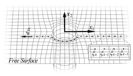
Figure 3. Indicative sparse mesh of the free surface boundary along with a cylindrical scatterer, highlighting the ξ-direction.

Based on the above Dawson–FD scheme [17], the additional non-square matrix $\partial U$ of dimensions $M_{FS}\times M$ is defined, whose elements

$$\partial U_{k,j}=A_k\cdot U_{k,j}+B_k\cdot U_{k-1,j}+C_k\cdot U_{k-2,j}+D_k\cdot U_{k-3,j},$$

(15)

account for the contribution of the j-element on $\partial U_k/\partial \xi$, at the k-collocation point on the free surface. Based on the above, the discrete model of the steady flow problem, modelling the disturbance field, is defined by the linear algebraic system of Equation (12), where:

$$A_{k,j}^{(S)}=\{\begin{array}{c}\partial U_{k,j}+\frac{g}{U_{\infty }^2}{W}_{k,j}\hspace{0.17em},\hspace{1em}\hspace{1em}Element\left(k\right)\in \partial D_{FS}\\ U_{k,j}\hspace{0.17em}{n}_{k,1}+V_{k,j}\hspace{0.17em}{n}_{k,2},\hspace{1em}Element\left(k\right)\in \partial D_{WS}\end{array}$$

(16a)

$$b_k^{(S)}=\{\begin{array}{c}0,\hspace{1em}\hspace{1em}\hspace{1em}Element\left(k\right)\in \partial D_{FS}\hspace{0.17em}\\ U_{\infty }\hspace{0.17em}{n}_{k,1},\hspace{1em}Element\left(k\right)\in \partial D_{WS}\end{array}$$

(16b)

After solving the above linear system, the free surface elevation is obtained from the dynamic boundary condition as:

$${\eta }_D^{(S)}\left(x\right)=\frac{U_{\infty }}{g}\frac{\partial {\phi }_D^{(S)}\left(x_1,x_2,0\right)}{\partial x_1},x\in \partial D_{FS}$$

(17)

which also approximates the free-surface elevation of the steady flow, noting that the set-down of the slow incident stream flow is very small and can be neglected.

2.3. Resulting Steady Flow Fields

Indicative results regarding the free surface elevation of the steady perturbation field are illustrated in Figure 4, for the case of a single cylinder of radius $R=0.15\hspace{0.17em}\mathrm{m}$, in a strip of constant depth equal to $h=1\hspace{0.17em}\mathrm{m}$, corresponding to an experimental setup in a tank, under the effect of a constant current flowing at speed $U_{\infty }=0.7\hspace{0.17em}\hspace{0.17em}\mathrm{m}/\mathrm{s}$ towards the negative $x_1$-direction, corresponding to bathymetric Froude number equal to $F_n=U_{\infty }/\sqrt{gh}=0.22$.

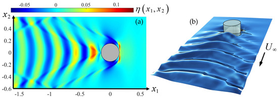
Figure 4. (a) Color plot and (b) rendered view of the free surface elevation generated by the steady perturbation field for one cylindrical scatterer of diameter $D=0.3\hspace{0.17em}\mathrm{m},\hspace{0.17em}h=1\hspace{0.17em}\mathrm{m},\hspace{0.17em}{U}_{\infty }=\left(-0.7,0,0\right)$.

Moreover, the present model can be extended for the study of any arrangement of cylindrical scatterers. As an example, Figure 5 illustrates the calculated steady perturbation field generated by a configuration consisting of four cylindrical scatterers, identical to the previous one, interacting with the same steady incident current in the waveguide of depth $h=1\hspace{0.17em}\mathrm{m}$. The centers of the scatterers’ circular sections (parallel to the plane $x_3=0),$ are located $0.8\hspace{0.17em}\mathrm{m}$ and $1.1\hspace{0.17em}\mathrm{m}$ apart in the $x_1$- and $x_2$-directions, respectively.

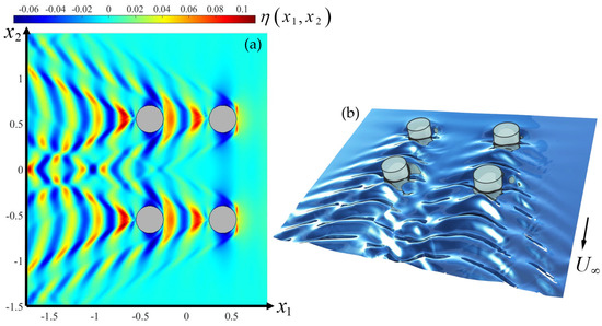
Figure 5. (a) Color plot and (b) rendered view of the free surface elevation generated by the steady perturbation field for four cylindrical scatterers of diameter $D=0.3\hspace{0.17em}\mathrm{m},\hspace{0.17em}h=1\hspace{0.17em}\mathrm{m},\hspace{0.17em}{U}_{\infty }=\left(-0.7,\hspace{0.17em}0,\hspace{0.17em}0\right)$.

In cases of slower current flows, characterized by F < 0.1, the wavelike pattern becomes very weak, and a useful approximation of the steady field on the free surface with the disturbance effect by the cylinders is obtained from a two-dimensional solution, corresponding to parallel flow over the cylinders. For example, in the case of the single cylinder and current flow of Figure 4, the following approximation can be used, exploiting standard results, for the disturbance potential:

$${\phi }_D^{(S)}\left(x_1,x_2,0\right)\approx \mathrm{Re}\left(-U_{\infty }{R}^2/z\right),\hspace{0.17em}\hspace{0.17em}\hspace{0.17em}z=x_1+i{x}_2,$$

(18)

and the above approximation provided by Equation (18) can be extended to include multiple cylindrical bodies.

2.4. Formulation of the 3D Wave Problem

For slow currents, the unsteady field associated with the wave flow can be calculated iteratively using, as a first approximation, the solution in the absence of the background current; see e.g., Belibassakis et al. [3].

In the case of waves without current, the incident field ${\phi }_I^{(U)}$ is given by

$${\phi }_I^{(U)}\left(x\right)=-\frac{igH}{2\omega }F\left(x_3\right)\exp \left[-i\hspace{0.17em}{k}_0^{(I)}\cdot R\right]\hspace{0.17em}$$

(19a)

where $F\left(x_3\right)={\cosh }^{-1}\left(k_{\hspace{0.17em}0}h\right)\cdot \cosh \left[k_{\hspace{0.17em}0}\left(x_{\hspace{0.17em}3}+h\right)\right]$ and $R$ is the position vector on the horizontal plane, $R\left(x\right)=x_{\hspace{0.17em}1}\cdot e{\hspace{0.17em}}_1+x_{\hspace{0.17em}2}\cdot e{\hspace{0.17em}}_2$, with $e{\hspace{0.17em}}_i,\hspace{0.17em}i=1,2$ denoting the unit vectors on the plane. The wavenumber $k_{\hspace{0.17em}0}$ is calculated as the root of the dispersion relation:

$${\omega }^{\hspace{0.17em}2}=k_{\hspace{0.17em}0}g\cdot \tanh \left(k_{\hspace{0.17em}0}\hspace{0.17em}h\right),$$

(19b)

and for incident waves propagating at an angle β, the wavevector $k_0^{(I)}\left(x\right)$ is defined by

$$k_0^{(I)}\left(x\right)=k_0\left[e_{\hspace{0.17em}1}\cdot \cos \left(\beta \right)+e_{\hspace{0.17em}2}\cdot \sin \left(\beta \right)\right].$$

(19c)

The problem concerning the diffraction field consists of the Laplace equation, combined with the linearized free surface boundary condition and impermeability conditions on the wetted surfaces of the cylinders and the seabed:

$${\nabla }^2{\phi }_D^{(U)}\left(x\right)=0,\hspace{0.17em}\hspace{0.17em}x\in D,\hspace{0.17em}$$

(20a)

$$\frac{\partial {\phi }_D^{(U)}\left(x\right)}{\partial \hspace{0.17em}{x}_3}-\mu \left(x;\omega \right)\hspace{0.17em}{\phi }_D^{(U)}\left(x\right)=0,\hspace{0.17em}\hspace{0.17em}x\in \partial D_{FS},$$

(20b)

$$\frac{\partial {\phi }_D^{(U)}\left(x\right)}{\partial n}=-\frac{\partial {\phi }_I^{(U)}\left(x\right)}{\partial n}\hspace{0.17em},\hspace{0.17em}\hspace{0.17em}x\in \partial D_{WS},$$

(20c)

$$\frac{\partial {\phi }_D^{(U)}\left(x\right)}{\partial n}=0,\hspace{0.17em}\hspace{0.17em}x\in \partial D_B,$$

(20d)

where $\mu \left(x;\omega \right)={\omega }^2/g$ is the frequency parameter, which is modified in the absorbing layer’s region, as described in the sequel.

2.4.1. Implementation of the Absorbing Layer Technique

For the satisfaction of an appropriate condition at infinity expressing the radiation of waves in the subcritical case, an absorbing layer (ABL) technique is adopted, consisting of a damping zone, surrounding the domain of interest; see, e.g., Bonovas et al. [18]. The latter is used to attenuate the outgoing scattered waves in an optimal way, preventing reflections from the outer boundary. For the implementation of the ABL, a rectangular frame is considered around the border of the domain on the free surface plane $x_{\hspace{0.17em}3}=0$. The thickness of the absorbing layer is selected to be of the order of the local wavelength $\lambda =2\pi /k_{\hspace{0.17em}0}$. Implementation of the ABL is achieved by modifying the frequency parameter inside the absorbing layer, as follows:

$$\mu \left(x;\omega \right)=\{\begin{array}{c}\hspace{1em}\hspace{1em}\hspace{1em}\frac{{\omega }^{\hspace{0.17em}2}}{g},\hspace{1em}\hspace{1em}\hspace{1em}\hspace{1em}\hspace{1em}\hspace{1em}\hspace{1em}R\left(x\right)<R_{PML}\left[\theta \left(x\right)\right]\\ \frac{{\omega }^{\hspace{0.17em}2}}{g}{\left[1+ic\frac{{\left|\hspace{0.17em}R\left(x\right)-R_{PML}\left[\theta \left(x\right)\right]\hspace{0.17em}\right|}^{\hspace{0.17em}n}}{{\lambda }^n}\right]}^{\hspace{0.17em}2},\hspace{0.17em}R\left(x\right)\ge R_{PML}\left[\theta \left(x\right)\right]\end{array}$$

(21)

where $R_{PML}\left[\theta \left(x\right)\right]$ denotes the PML activation radius in the direction $\theta \left(x\right)={\tan }^{-1}\hspace{0.17em}\left(x_{\hspace{0.17em}2}/x_{\hspace{0.17em}1}\right)$, while c and the exponent $n$ are parameters depending on the angular frequency $\omega$, that have been optimized in previous work concerning similar scattering problems; see Bonovas et al. [18]. The BVP described by Equations (20a)–(20d) is numerically solved using a low-order BEM with a piecewise constant normal-dipole singularity distribution on four-node quadrilateral elements equivalent to vortex rings. In this case, the induced quantities associated with each element’s contribution to a collocation point are analytically calculated, based on the equivalence of the 3D constant-strength doublet element to a vortex ring, surrounding the panel around its edges [15]. Finally, the free surface elevation is obtained from the solution ${\phi }^{(U)}={\phi }_I^{(U)}+{\phi }_D^{(U)}$ as follows:

$${\eta }^{(U)}\left(x\right)=-\frac{i\omega }{g}{\phi }^{(U)}\left(x_1,x_2,0\right),\hspace{0.17em}x\in \partial D_{FS}$$

(22)

An indicative result of the diffraction field (real and imaginary part) without current effects is illustrated in Figure 6a,b, concerning a single cylinder of radius $R=0.15\hspace{0.17em}\mathrm{m}$, located in a waveguide of constant depth equal to $h=1\hspace{0.17em}\mathrm{m}$. In this case, the wave height of the incident field is $H=0.2\hspace{0.17em}\mathrm{m}$ and the corresponding wavelength is $\lambda =1.2\hspace{0.17em}\mathrm{m}.$ The direction of propagation of the incident field is considered to be collinear to the velocity of the background current of Figure 4 directed along the negative x₁-axis $(\beta =\pi )$.

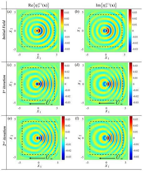
Figure 6. Incident waves of wavelength and height $\lambda =1.2\hspace{0.17em}\mathrm{m},\hspace{0.17em}H=0.2\hspace{0.17em}\mathrm{m}$ interacting with a vertical cylinder of diameter D = 0.3 m in water depth h = 1 m, in the presence of a parallel flow current $U_{\infty }=\left(-0.3\hspace{0.17em}\mathrm{m}/\mathrm{s},0,0\right)$. (a,b) Imaginary and real part of the initial estimation of the disturbance field and corrected patterns after the first iteration (c,d) and after the second iteration (e,f), respectively. The dashed line indicates the absorbing layer region.

2.4.2. An Iterative Scheme for the Additional Scattering Effect Due to Current

In order to take into account the additional effects of the current on the wave scattering, the directional wavenumber $k_0^{(D)}\left(x\right)$ involved in the formulation of the wave diffraction problem is iteratively estimated using the gradient of the phase of the c function ${\phi }_D^{(U)}$:

$$k\left(x\right)={\nabla }_h\left(S_D^{(U)}\left(x\right)\right),\hspace{0.17em}{S}_D^{(U)}\left(x\right)=\ln \left[\frac{{\phi }_D^{(U)}\left(x\right)}{\left|{\phi }_D^{(U)}\left(x\right)\right|}\right].$$

(23)

The developed iterative scheme is based on the redefinition of the local intrinsic frequency $\sigma \left(x\right)$ of the diffracted field ${\phi }_D^{(U)}$, as modified by the background flow. The local intrinsic frequency is calculated by:

$$\sigma \left(x\right)=\omega -\left[k\left(\widehat{k}\cdot U^{(S)}\right)\right],$$

(24)

where $U^{(S)}\left(x\right)={\nabla }_h\left({\phi }_I^{(S)}+{\phi }_D^{(S)}\right),\hspace{0.17em}x\in \partial D_{FS}$ is the free-surface velocity field generated by the steady background current, $\widehat{k}\left(x\right)=k/\left|k\right|$ is the unit wavevector, with a direction defined by Equation (23) and $k\left(x\right)$ is the local wavenumber, calculated by the modified dispersion relation, which also accounts for the presence of the current, as follows:

$$\sigma \left(x\right)=\omega -\left[k\left(\widehat{k}\cdot U^{(S)}\right)\right]=\sqrt{k\hspace{0.17em}g\cdot \tanh \left(kh\right)}.$$

(25)

Subsequently, the linear system resulting from the BEM discretization of Equations (20a)–(20d) and (21) is solved, using the local intrinsic frequency $\sigma \left(x\right)$ on $\partial D_{FS}$ including the absorbing layer. In each iterative step the incident wave field is:

$${\phi }_I^{(U)}\left(x\right)=-\frac{igH}{2{\sigma }_I}F\left(x_3\right)\exp \left[-i\hspace{0.17em}{k}_0^{(I)}\left(x\right)\cdot R\right],$$

(26a)

with $F\left(x_3\right)={\cosh }^{-1}\left(k_0^{(I)}h\right)\cosh \left[k_0^{(I)}\left(x_{\hspace{0.17em}3}+h\right)\right]$, and $k_0^{(I)}$ is calculated as the root of the dispersion relation:

$${\sigma }_{{\rm I}}^2\equiv {\left(\omega -k_0^{(I)}{U}_{\infty }\right)}^2=k_0^{(I)}g\cdot \tanh \left(k_0^{(I)}\hspace{0.17em}h\right).$$

(26b)

Indicative results of the modified diffraction field (real and imaginary part) are illustrated in Figure 6 concerning the diffraction wave field by a single cylinder in the presence of a background steady current, with velocity $U_{\infty }=0.25\hspace{0.17em}\mathrm{m}/\mathrm{s}$ flowing towards the negative $x_1$-direction. In Figure 6, we observe the change of the wavelength in the upwave and downwave regions due to the Doppler effect of the current, as well as the fact that the present iterative scheme converges very fast to the final solution.

Furthermore, the 3D BEM for the calculation of the unsteady field can also be extended to treat more general arrangements of cylindrical scatterers. Indicative results are illustrated in Figure 7, concerning the diffracted and the total unsteady field generated by a configuration consisting of four cylindrical scatterers of radius $R=0.15\hspace{0.17em}\mathrm{m}$, in the waveguide of depth $h=1\hspace{0.17em}\mathrm{m}$. The centers of the scatterers’ circular sections (parallel to the plane $x_3=0$), are located $0.8\hspace{0.17em}\mathrm{m}$ and $1.1\hspace{0.17em}\mathrm{m}$ apart in the $x_1$- and $x_2$-directions, respectively.

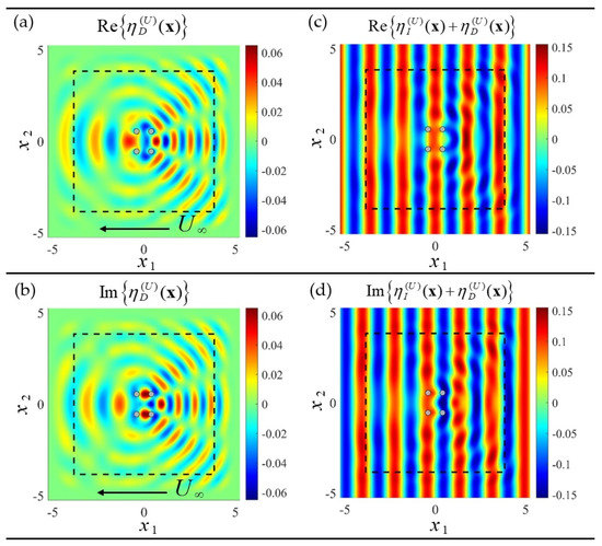
Figure 7. Incident waves of wavelength and height $\lambda =1.2\hspace{0.17em}\mathrm{m},\hspace{0.17em}H=0.1\hspace{0.17em}\mathrm{m}$ interacting with an arrangement of four cylindrical scatterers of diameter D = 0.3 m in water depth h = 1 m, in the presence of a collinear following current $U_{\infty }=\left(-0.25\hspace{0.17em}\mathrm{m}/\mathrm{s}\hspace{0.17em},0,0\right)$, indicated with an arrow. (a,b) Real and imaginary part of free surface elevation of the diffracted and (c,d) the total unsteady field, respectively. The dashed line indicates the absorbing layer region.

The wave height of the incident field is again $H=0.2\hspace{0.17em}\mathrm{m}$ and the wavelength (of the initial field) is $\lambda =1.2\hspace{0.17em}\mathrm{m}$. The direction of propagation of the incident field is $\beta =\pi$. The subplots in the first column of Figure 7 illustrate the diffracted field, while the total unsteady field is shown in the right column subplots, respectively, as calculated by the previously described iterative scheme, showing the modifications induced by the uniform background current propagating at speed $U_{\infty }=0.25\hspace{0.17em}\mathrm{m}/\mathrm{s}$ towards the negative $x_1$-direction.

In Figure 7, we observe the strong modification of the wave field due to multiple interactions by the scatterers and the current, leading to the generation of reflection beams, in addition to the Doppler effect due to the current, that is clearly presented in the far upwave and downwave regions.

3. A Simplified 2D Formulation on the Horizontal Plane

As stated earlier, in cases of slow current flows, characterized by bathymetric Froude number $F_n=U_{\infty }/\sqrt{gh}<0.1$, the wavelike pattern downstream the cylinders becomes quite small. Furthermore, for such currents there is a significant decrease in the Kelvin pattern’s wavelength, resulting in waves of the order of a few millimeters in length. Taking into account that the proposed 3D BEM necessitates a minimum of 15 elements per wavelength on the free surface in order to represent the flow, we conclude that the model leads to excessive mesh size requirements. For this purpose, in this section, a simplified 2D formulation on the horizontal plane is developed using a coupled BEM–FEM approach overcoming the above limitations. In addition, having in mind possible applications of wave–current-body interaction problems in channels and in experimental studies in wave flumes, we consider a water tank of a constant depth equal to $h,$ where an arrangement of rigid cylinders with diameter $d=2a$ is confined between two parallel vertical side walls. The same Cartesian coordinate system as before is used, with the $x_3$-axis pointing upwards and $x_h=\left(x_1,x_2\right)$ spanning the mean water level plane $(\mathrm{at}\hspace{0.17em}\hspace{0.17em}{x}_3=0)$. The tank’s width is equal to B and the water body is bounded by vertical sidewalls. Let the bounded region $D_h\subset {ℝ}^2$ represent the calm free surface plane of the water, containing the configuration of cylinders. The horizontal domain, again denoted by $D$, has length L and is bounded by the vertical sidewalls at $x_2=\mp B/2$ and two fictitious lateral boundaries at $x_{\hspace{0.17em}1}=\mp L/2$. Τhe free surface of the water is also interrupted by the projections of the cylinders’ cross sections on the $x_{\hspace{0.17em}1\hspace{0.17em}}{x}_{\hspace{0.17em}2}$-plane; see Figure 8. As before, the fluid motion is considered to be fully described by the potential function $\Phi \left(x,x_3\hspace{0.17em};t\right)$, whose gradient is equal to the fluid’s velocity:

$$v\left(x\hspace{0.17em};t\right)=\nabla \Phi \left(x_h,x_3\hspace{0.17em};t\right),\hspace{0.17em}{x}_h\in D,\hspace{0.17em}-h<x_3<0.$$

(27)

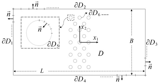
Figure 8. Indicative boundary mesh of $\partial D$.

The flow variables are again decomposed into a steady background flow and the time-dependent wave part, which are, respectively, described by a steady and an unsteady potential function, while harmonic time dependence is considered for the unsteady problem; thus,

$$\Phi \left(x_h,x_3\hspace{0.17em};t\right)={\Phi }^{(S)}\left(x_h,x_3\right)+{\Phi }^{(U)}\left(x_h,x_3\hspace{0.17em};t\right),$$

(28a)

$${\Phi }^{(U)}\left(x_h,x_3\hspace{0.17em};t\right)=\mathrm{Re}\left\{\phi \left(x_h,x_3\right)\exp \left(-i\hspace{0.17em}\omega \hspace{0.17em}t\right)\right\},$$

(28b)

where $\omega$ is the absolute frequency of the incident wave field.

3.1. Formulation of the Steady Current Problem

The steady background current is defined by the interaction of a uniform flow parallel to the $x_{\hspace{0.17em}1}$-axis, $U_{\infty }$, with the cylinders in the constant depth domain. Under the assumption of incompressibility, the continuity equation reduces to the Laplace equation for the potential function ${\Phi }^{(S)}(x)$. The boundary $\partial D$ is decomposed in $4+N_C$ sections, where $N_C$ is the number of cylinders in the considered arrangement, as presented in Figure 8. The flow entrance and exit are denoted as $\partial D_1$ and $\partial D_3,$ respectively, and the sidewalls are denoted by $\partial D_2$ and $\partial D_4$. Finally, the vertical rigid walls of the cylinders are represented by $\partial D_C={\displaystyle {\cup }_{n=5}^{N_C+4}\partial D_n}$.

The corresponding 3D steady field can be evaluated as a solution to the BVP described by Equations (10a)–(10d). However, for slow inflow current velocity $U_{\infty }<<\min (\sqrt{gh},\sqrt{gR})$, the Neumann–Kelvin free-surface boundary condition (Equation (10b) reduces to:

$$\frac{\partial {\Phi }^{(S)}}{\partial x_3}=0,\hspace{0.17em}\hspace{0.17em}\hspace{0.17em}{x}_3=0.$$

(29a)

Taking into account the same (homogeneous Neumann) condition on the seabed,

$$\frac{\partial {\Phi }^{(S)}}{\partial x_3}=0,\hspace{0.17em}\hspace{0.17em}\hspace{0.17em}{x}_3=-h,$$

(29b)

and the fact that the side walls of the cylinders are vertical, the flow field is approximately constant in the vertical direction and, thus, ${\Phi }^{(S)}\left(x_h,x_3\right)\approx {\Phi }^{(S)}\left(x_1,x_2\right)$. Under the additional assumption that the steady perturbation field has died out near the vicinity of the lateral boundaries located at $x_{\hspace{0.17em}1}=\mp L/2$, the steady potential function ${\Phi }^{(S)}(x)$ can be approximated as a solution to the following BVP on the $x_1\hspace{0.17em}{x}_2$-plane:

$${\nabla }^2{\Phi }^{(S)}\left(x_h\right)=0,\hspace{0.17em}\hspace{0.17em}{x}_h\in D,\hspace{0.17em}$$

(30a)

$$\frac{\partial {\Phi }^{(S)}\left(x_h\right)}{\partial n}=0,\hspace{1em}{x}_h\in \left(\partial D_2\cup \partial D_4\cup \partial D_c\right),$$

(30b)

$$\frac{\partial {\Phi }^{(S)}\left(x_h\right)}{\partial x_1}\approx U_{\infty }\hspace{0.17em},\hspace{0.17em}\hspace{0.17em}{x}_h\in \left(\partial D_1\cup \partial D_3\right),$$

(30c)

where Equation (30c) is an approximation, stating that the flow in the inlet and outlet sections $\partial D_1$ and $\partial D_3$ is uniform and parallel to the x₁-axis. The numerical solution to the above problem is obtained using boundary integral equation formulations, based on the single-layer potential; see also Belibassakis et al. [4]. This is achieved by introducing the following integral representation for the steady potential function in D:

$${\Phi }^{(S)}\left(x\right)={\displaystyle \underset{\partial D}{\int }\mu \left(x^{\prime }\right)G\left(x^{\prime },x\right)d\ell \left(x^{\prime }\right)},x\in D\hspace{0.17em},x^{\prime }\in \partial D,$$

(31)

where $G\left(x^{\prime },x\right)=\ln \left|x^{\prime }-x\right|/2\pi$, $\mu (x^{\prime }),\hspace{0.17em}\hspace{0.17em}{x}^{\prime }\in \partial D$ is a source density distribution, defined on the boundary of the domain D and $d\ell \left(x^{\prime }\right)$ denotes the differential element along $\partial D$. Based on Equation (31), the normal derivatives of ${\Phi }^{(S)}(x)$, taking into account that the normal vector on $\partial D$ is directed towards the exterior of the domain, reduce to the following equation (see, e.g., Kress [19]):

$$\frac{\partial {\Phi }^{(S)}\left(x_h\right)}{\partial n}={\displaystyle \underset{\partial D}{\int }\mu \left(x_h^{\prime }\right)\frac{\partial G\left(x_h^{\prime },x_h\right)}{\partial n}d\ell \left(x_h^{\prime }\right)}-\frac{\mu \left(x_h\right)}{2}\hspace{0.17em},\hspace{1em}\left(x_h,x_h^{\prime }\right)\in \partial D.$$

(32)

A low-order 2D BEM approach based on simple (Rankine) sources, combined with a collocation technique, is used to derive numerical solutions of the above problem. The boundary is approximated using linear segments on which the source distribution is assumed to be piecewise constant [15] and the boundary integrals expressing each segment’s contribution to a collocation point are analytically calculated. Moreover, the collocation points, where the corresponding equations are satisfied, are chosen to coincide with the linear segments’ midpoints. Thus, the boundary integral equations reduce to an algebraic system, which can be solved to determine the piecewise constant values of the vector ${\left\{{\mu }_k\right\}}_{k=1}^M,\hspace{0.17em}M$, being the number of boundary elements used to approximate the geometry of $\partial D$.

As an indicative solution of the above 2D problem, the case of a porous structure tested in a flume, studied by Belibassakis et al. [4], is examined, as illustrated in Figure 9.

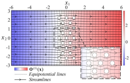
Figure 9. Equipotential lines and streamlines of the steady field resulting from the interaction of a current propagating along the $x_{\hspace{0.17em}1}$ axis at speed $U_{\infty }=0.5\hspace{0.17em}\mathrm{m}/\mathrm{s}$ with a configuration of 23 cylinders of radius $a=0.15\hspace{0.17em}\mathrm{m}$ in a 6 m wide tank.

In particular, an arrangement of 23 cylinders with radius $R=0.15\hspace{0.17em}\mathrm{m}$, interacting with a uniform current flowing towards the positive $x_{\hspace{0.17em}1}$-axis, with speed $U_{\infty }=0.5\hspace{0.17em}\mathrm{m}/\mathrm{s}$, is considered. For low current speed, the 2D approach provides reasonable prediction of the flow characteristics, while it has very low computational cost.

3.2. Formulation of the Wave Propagation Problem on the Horizontal Plane

Restricting ourselves to small-amplitude waves, the harmonic wave field in the region of interest is approximated by keeping only the propagating mode in the representation of the wave potential in the constant depth strip, as follows:

$${\Phi }^{(U)}\left(x_h,x_3\hspace{0.17em};t\right)\approx \mathrm{Re}\left\{-\frac{igA}{\omega }\phi \left(x_h\right)F\left(x_3\right)\exp \left(-i\hspace{0.17em}\omega \hspace{0.17em}t\right)\right\},$$

(33)

where $F\left(x_3\right)={\cosh }^{-1}\left(k_{\hspace{0.17em}0}h\right)\cdot \cosh \left[k_{\hspace{0.17em}0}\left(x_{\hspace{0.17em}3}+h\right)\right]$, $A$ = H/2 is the wave amplitude, and $k_{\hspace{0.17em}0}$ is the wavenumber, obtained as the solution of the dispersion relation (Equation (19b)). Using Equation (33) in the Laplace equation, we obtain

$$\left({\nabla }_h^2\hspace{0.17em}+k_0^2\right)\hspace{0.17em}\phi (x_h)=0,\hspace{0.17em}\hspace{0.17em}{x}_h\in D,$$

(34)

where ${\nabla }_h=(\partial /\partial x_{\hspace{0.17em}1},\hspace{0.17em}\partial /\partial x_{\hspace{0.17em}2})$ is the horizontal gradient. Therefore, in the absence of currents, the complex wave field $\phi \left(x\right)$ on the free surface is obtained as a solution to the Helmholtz equation (Equation (34)). The latter’s coefficient is defined by the dispersion relation and appropriate boundary conditions apply to the boundaries as follows:

On the tank’s side walls, at $x_2=\mp B/2$ and on the cylinders’ boundaries:

$$\frac{\partial \phi \hspace{0.17em}(x)}{\partial n}\hspace{0.17em}=0,\hspace{0.17em}\hspace{0.17em}x\in \left(\partial D_{\hspace{0.17em}2}\cup \partial D_{\hspace{0.17em}4}\cup \partial D_C\right).$$

(35)

At the entrance and outlet boundaries, $x_1=\mp L/2,$ appropriate wave entry and radiation conditions need to be defined. The first one, at $x_1=-L/2$ is derived by assuming a parallel plane incident wave directed along the x₁-axis, which is partially reflected due to the structure; thus, ${\phi \left(x_h\right)|}_{x_1=-L/2}=\exp \left(i{k}_0{x}_1\right)+R\exp \left(-i{k}_0{x}_1\right)$, where $R$ denotes the reflection coefficient. Subsequently, by differentiating with respect to $x_1$ and eliminating $R$, we obtain the following mixed-type condition, that is used on the entrance boundary $\partial D_{\hspace{0.17em}1}$:

$$\frac{\partial \phi (x_h)}{\partial n}-i{k}_0\hspace{0.17em}\phi (x_h)=-2A\hspace{0.17em}\mathrm{i}{k}_0\exp \left(-\mathrm{i}{k}_0\hspace{0.17em}L/2\right),\hspace{0.17em}\hspace{0.17em}{x}_h\in \partial D_1\hspace{0.17em}.$$

(36)

On the exit boundary, an absorbing boundary condition is used by employing an optimal Perfectly Matched Layer; see Karperaki et al. [20]. Similar PML techniques have been developed for the numerical treatment of wave propagation and scattering problems over general seabed topographies; see Belibassakis et al. [21] and the references cited therein.

In order to ensure radiation of the solution at the outlet boundary, a PML reformulation of Equation (34) is considered. Assuming a layer of finite thickness $\theta$, the domain of interest is extended as $\stackrel{⌢}{D}=D\cup D_{PML}$, where:

$$D_{PML}=\left[L/2,\hspace{0.17em}L/2+\theta \right]\times \left[-B/2,\hspace{0.17em}B/2\right].$$

(37)

The absorbing layer is constructed so as to attenuate the waves in the PML zone ${\phi }^{(*)}\in D_{PML}$ rapidly, with minimum backscattering, leaving intact the numerical solution $\phi \in D$. This is achieved by employing a coordinate stretching, using the transformation function $\gamma \left(x_1,x_2\right)$:

$$\gamma \left(x\right)=\{\begin{array}{c}\hspace{0.17em}\hspace{1em}1,\hspace{0.17em}\hspace{1em}(x_1,x_2)\in D\\ 1+i\frac{\sigma \left(x_1\right)}{k_0},\hspace{0.17em}\hspace{0.17em}\hspace{0.17em}(x_1,x_2)\in D_{PML}\end{array},$$

(38a)

where $\sigma (x_{\hspace{0.17em}1})$ is the absorbing function, controlling the attenuation rate in the PML. Following Karperaki et al. [20], an unbounded absorbing function is employed in Equation (38a) to ensure parameter-free and optimal solution decay; thus,

$$\sigma \left(x_1\right)=\frac{1}{\left(L/2+\theta \right)-x_1},\hspace{0.17em}\hspace{0.17em}\hspace{0.17em}(x_1,x_2)\in D_{PML}.$$

(38b)

Notably, the employed unbounded absorbing function Equation (38b) allows for a thin layer, approximately 2% of the characteristic wavelength, suggesting minimal computational cost. In the extended region, the governing equation becomes:

$$\frac{\partial }{\partial x_1}\left({\gamma }^{-1}\frac{\partial \phi }{\partial x_1}\right)+\frac{\partial }{\partial x_2}\left(\gamma \hspace{0.17em}\frac{\partial \phi }{\partial x_2}\right)+k^2\gamma \phi =0,\hspace{0.17em}\hspace{0.17em}x\in \stackrel{⌢}{D}.$$

(39)

It is worth noticing here that the above PML technique could be easily extended to also apply to the transverse boundaries in order to treat the same interaction–scattering problem in the unbounded horizontal plane.

3.3. An FEM for the Wave Propagation–Scattering Problem

For the numerical solution of the above problem on the horizontal plane, and taking into account that the wavenumber parameter $k_0^2(x_h)$ involved in the field Equation (34) is spatially variable due to the current effect, a conforming finite element scheme is employed for the numerical solution. Considering the weight functions $w\in H^1(\stackrel{⌢}{D})$, the weak form is derived by multiplying Equation (34) with $w(x_h)$ and integrating over the domain. Subsequently, performing integration by parts and imposing the boundary conditions results in:

$$\begin{array}{l}-{\displaystyle \underset{\stackrel{⌢}{D}}{\int }{\nabla }_{h}w\cdot }\gamma \hspace{0.17em}d\stackrel{⌢}{D}+{\displaystyle \underset{\stackrel{⌢}{D}}{\int }{k}^{2}w\gamma \phi }\hspace{0.17em}d\stackrel{⌢}{D}+{\displaystyle \underset{x_2=-B/2}{\overset{x_2=B/2}{\int }}w\left(-L/2,x_2\right)}\left(I-ik\hspace{0.17em}\phi \right)ds+\\ \hspace{0.17em}\hspace{0.17em}\hspace{0.17em}\hspace{0.17em}\hspace{0.17em}\hspace{0.17em}\hspace{0.17em}\hspace{0.17em}\hspace{0.17em}\hspace{0.17em}\hspace{0.17em}\hspace{0.17em}\hspace{0.17em}\hspace{0.17em}\hspace{0.17em}\hspace{0.17em}\hspace{0.17em}\hspace{0.17em}\hspace{0.17em}\hspace{0.17em}\hspace{0.17em}\hspace{0.17em}\hspace{0.17em}\hspace{0.17em}\hspace{0.17em}\hspace{0.17em}\hspace{0.17em}\hspace{0.17em}\hspace{0.17em}\hspace{0.17em}\hspace{0.17em}\hspace{0.17em}+{\displaystyle \underset{x_2=-B/2}{\overset{x_2=B/2}{\int }}n\cdot \left(w\left(L/2+\theta ,x_2\right)\hspace{0.17em}{\gamma |}_{x_1=L/2+\theta }\right)\hspace{0.17em}}\hspace{0.17em}ds=0\hspace{0.17em}.\end{array}$$

(40)

where $I=2\mathrm{i}{k}_0\exp \left(-\mathrm{i}{k}_{0}L/2\right)$, and $\gamma$ denotes the following vector field:

$$\gamma =\left({\gamma }^{-1}\frac{\partial \phi }{\partial x_1},\gamma \hspace{0.17em}\frac{\partial \phi }{\partial x_2}\right).$$

(41)

A Delaunay-based triangular partitioning is employed for the region of interest, while a regular triangular mesh is employed for the PML region, as shown in Figure 10. For the solution of Equation (40), linear triangular elements are employed; thus, the approximate solution in each element is written as:

$${\phi }_e^h\left(x_1,x_2\right)={\displaystyle \sum _{i=1}^3{N}_i}{\phi }_i=N\hspace{0.17em}\mathsf{\phi }\hspace{0.17em}$$

(42)

where $\mathsf{\phi }$ denotes the vector of nodal unknowns and $N$ is the vector containing the linear shape functions associated with the triangular elements. Thus, the discrete weak form expressed for each K-element of the subdivision of the domain is written in terms of the nodal unknowns as follows:

$$\begin{array}{l}-{\displaystyle \underset{K}{\int }{\left(N_{,x_1}\right)}^{\mathrm{T}}\hspace{0.17em}{\gamma }^{-1}}\left(N_{,x_1}\right)\hspace{0.17em}\mathsf{\phi }\hspace{0.17em}d\stackrel{⌢}{D}-{\displaystyle \underset{K}{\int }{\left(N_{,x_2}\right)}^{\mathrm{T}}\hspace{0.17em}\gamma }\left(N_{,x_2}\right)\hspace{0.17em}\mathsf{\phi }\hspace{0.17em}d\stackrel{⌢}{D}\hspace{0.17em}+\\ \hspace{0.17em}\hspace{0.17em}\hspace{0.17em}\hspace{0.17em}\hspace{0.17em}\hspace{0.17em}\hspace{0.17em}\hspace{0.17em}\hspace{0.17em}\hspace{0.17em}\hspace{0.17em}\hspace{0.17em}\hspace{0.17em}\hspace{0.17em}\hspace{0.17em}\hspace{0.17em}\hspace{0.17em}\hspace{0.17em}\hspace{0.17em}\hspace{0.17em}\hspace{0.17em}\hspace{0.17em}\hspace{0.17em}\hspace{0.17em}\hspace{0.17em}\hspace{0.17em}\hspace{0.17em}\hspace{0.17em}\hspace{0.17em}+{\displaystyle \underset{K}{\int }{k}_0^2\hspace{0.17em}\gamma \hspace{0.17em}{N}^{\mathrm{T}}N\hspace{0.17em}\mathsf{\phi }}\hspace{0.17em}d\stackrel{⌢}{D}-i{\displaystyle \underset{\partial K}{\int }k\hspace{0.17em}{N}^{\mathrm{T}}N\hspace{0.17em}\hspace{0.17em}\mathsf{\phi }}\hspace{0.17em}ds=g,\end{array}$$

(43a)

where

$$g=-I{\displaystyle \underset{x_2=-B/2}{\overset{x_2=B/2}{\int }}w\left(-L/2,x_2\right)}\hspace{0.17em}ds\hspace{0.17em}\hspace{0.17em}\hspace{0.17em}.$$

(43b)

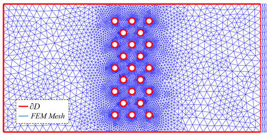
Figure 10. Indicative plot of Delaunay triangulation-based mesh of $D$, augmented by a regular triangular mesh in the PML region.

Upon assembly, the final FEM system in terms of the global unknowns $Q$ (the global collection of nodal values associated with the field approximation) is finally obtained:

$$K\hspace{0.17em}Q=G,$$

(44)

with $G$ being the forcing vector, obtained from the global collection of elemental forcing terms $(g)$ and $K$ being the global stiffness matrix.

3.4. Iterative Scheme

Similarly, as in the 3D case examined in Section 2, the refraction–diffraction effect of the current on the wave field is evaluated by considering the vector wavenumber $k\left(x_h\right)$, the modulus of which $(k_0=|k|)$ is the parameter of the field equation of the propagation problem in Equations (34) and (39). Again, by using the representation:

$$\phi \left(x_h\right)=F\left(x_h\right)\exp \left(iS\left(x_h\right)\right)$$

(45a)

where $F(x)$ denotes the complex modulus and $S(x)$ the phase of the wave potential $\phi$ on the surface, the directional wavenumber in $D$ equals:

$$k\left(x\right)={\nabla }_h\left(S\left(x\right)\right),\hspace{0.17em}\hspace{0.17em}\hspace{0.17em}S\left(x\right)=\ln \left[{\left|\phi \left(x\right)\right|}^{-1}\phi \left(x\right)\right].$$

(45b)

The developed iterative scheme is based on the redefinition of the local wavenumber $k(x_1,x_2)$, which, in turn, defines the local intrinsic frequency $\sigma (x_h)$ of the wavefield, as modified by the steady flow. The local frequency equals:

$$\sigma \left(x_h\right)=\omega -\left[k\left(\widehat{k}\hspace{0.17em}{U}^{(S)}\right)\right],\hspace{0.17em}\hspace{0.17em}\hspace{0.17em}$$

(46)

where $U^{(S)}\left(x_h\in D\right)={\displaystyle \underset{\partial D}{\int }\mu \left(x_h^{\prime }\right)\hspace{0.17em}\cdot \nabla G\left(x_h^{\prime },x\right)d\ell \left(x_h^{\prime }\right)}$ is the velocity field generated by the steady background current (as calculated by the 2D BEM described in the Section 3.1), $\widehat{k}\left(x\right)=k/\left|k\right|$ is the unit wavevector with a direction defined by Equation (45b), and $k\left(x_h\right)=k_0$ is the local wavenumber that is obtained using the modified dispersion relation Equations (19a)–(19c) taking into account the effects of the local current:

$$\sigma \left(x_h\right)=\sqrt{k_0{\left(x_h\right)}_{\hspace{0.17em}}g\tanh \left[k_0\left(x_h\right)h\right]}.$$

(47)

Based on the above, the solution of the wave problem is again obtained by iterations and the local direction of the wavenumber along with its modulus are calculated at each step. Subsequently, the field is obtained from the numerical solution of the resulting linear system (Equation (44)), from which a renewed prediction of the wavenumber vector field is calculated via the horizontal gradient of the phase $S\left(x_h\right)$. This procedure continues until consecutive iterations bear no additional transformations.

4. Numerical Results

In this section numerical results are presented for the verification of the simplified numerical scheme on the horizontal plane and demonstration of the applicability of the model.

4.1. Verification of the FEM Scheme without Current

We first consider the wave propagation problem, in the absence of current, which is governed by the Helmholtz equation with a constant coefficient $k_0$, provided by the root of the dispersion relation (Equation (19b)). This problem can also be treated by means of boundary integral representations, by exploiting the Green’s Function of the Helmholtz equation in 2D, as presented by Belibassakis et al. [4], and the numerical results are compared against the solution obtained by the present the FEM scheme. In particular, a numerical wave tank configuration is considered, containing a symmetrical array in a finite subregion modelling a porous structure consisting of multiple vertical bottom-seated vertical cylinders, as shown in Figure 11, and the transformation of the wave field by the considered configuration is examined.

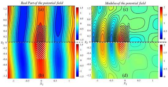
Figure 11. Real part and modulus of the symmetric wave field in the waveguide of water depth h = 0.23 m, at frequency $f=1\hspace{0.17em}\mathrm{H}\mathrm{z}$, as calculated by (a,c) the modal BEM developed by Belibassakis, et al. [4] and (b,d) the present FEM scheme.

Figure 11 depicts the real part of the calculated wave field, generated by the interaction of an arrangement consisting of $N_c=148$ cylinders of radius $R=0.016\hspace{0.17em}\mathrm{m}$ (porous breakwater) with an incident wave field of frequency $f=1\hspace{0.17em}\mathrm{Hz}$ in a 10 m long and 2.6 wide flume. The porous structure is modelled by arranging seventeen rows of four cylinders and placing a series of five cylinders between two consecutive four cylinder-rows. The overall layout is contained in a rectangle of dimensions $[L\times B]=[0.3\hspace{0.17em}\mathrm{m}\times 1.2\hspace{0.17em}\mathrm{m}]$ and, thus, the porosity of this arrangement is equal to ${\gamma }_p=1-N_c\pi R^2/\left(LB\right)=0.67$; see also Belibassakis et al. [4].

In particular, in the lower part of Figure 11b, the present FEM solution of the symmetric field near the porous structure is plotted and compared against the corresponding BEM solution, that is included in the upper half of the Figure 11a, where in both subplots, only the half-symmetric field is shown. Similarly, Figure 11c,d depicts the modulus of the potential field for the same case as before, as calculated by the BEM and the proposed FEM scheme.

The FEM results of the Figures are based on a discretization of 487,952 triangular elements for the whole domain, 603 of which are located in the PML region. As can be observed in this figure, the results of the two methods show very good agreement, verifying the present FEM scheme in the case of wave interaction with complex structures consisting of multiple vertical cylinders, as in the case of such systems operating as porous breakwaters.

4.2. Verification of the Present FEM in the Case of Waves and Currents

First, the case of waves only (without current) is considered. In Figure 12b, the present FEM solution is compared against the corresponding 3D BEM solution on the free-surface shown in Figure 12a, where again only the half-symmetric field is shown. In this case, a single cylinder of radius $R=0.3\hspace{0.17em}\mathrm{m}$ interacts with an incident wave field of frequency $f=1\hspace{0.17em}\mathrm{Hz},$ in water depth $h=1\hspace{0.17em}\mathrm{m}$. The resulting wavelength is $\lambda =1.56\hspace{0.17em}\mathrm{m}$. The BEM results are calculated on a 3D structured boundary mesh, based on quadrilateral elements (see Section 2). The free surface part of the mesh is generated by defining 24 nodes per wavelength in both horizontal directions, modelling a square domain of dimension $3.2\lambda$ with 23,700 elements. In this case, a $1.2\lambda$ thick absorbing layer is used to attenuate the diffracted outgoing wavefronts, in order to avoid backscattering.

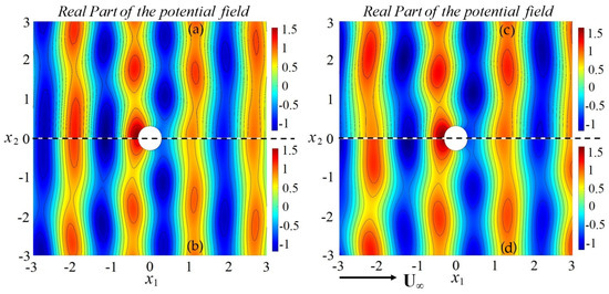
Figure 12. Real part of the symmetric field on the horizontal plane, in water depth h = 1 m, for a wave at frequency $f=1\hspace{0.17em}\mathrm{H}\mathrm{z}$, interacting with a cylinder of radius 0.3 m without current, as calculated by (a) the 3D BEM and (b) the proposed 2D FEM scheme. Calculated field for waves of the same frequency and height in the presence of a current of speed $U_{\infty }=0.1\hspace{0.17em}\mathrm{m}/\mathrm{s}$ as calculated by (c) the present 3D BEM and (d) the proposed 2D coupled BEM–FEM scheme.

The present FEM results are based on a 2D mesh consisting of 60,447 triangular elements on the horizontal plane, 1567 of which are in the absorbing layer of thickness $0.02\lambda$. Since the proposed FEM scheme was developed to simulate wave phenomena in a tank, a square domain of side length $12\lambda$ was considered in order to minimize reflection effects from the sidewalls. As depicted in Figure 12, the results of the two methods are compatible, verifying the proposed scheme. Next, the same configuration is considered with waves of the same frequency and a uniform following current, flowing along the $x_{\hspace{0.17em}1}$-axis at a small speed $U_{\infty }=0.1\hspace{0.17em}\mathrm{m}/\mathrm{s}$. Figure 12c,d illustrates the comparison of the wave field on the free surface as calculated by the present two methods: 3D BEM (upper subplot) and FEM on the horizontal plane (lower, subplot), respectively. In this case results are plotted after five iterations, which are found to be enough for numerical convergence as discussed in the sequel.

As can be seen in the above Figures, both models predict the increase in the wavelength due to the following current, whose theoretical value is $\lambda =1.78\hspace{0.17em}\mathrm{m}$, based on the modified dispersion relation (Equation (47)). Minor differences are observed between the two methods, mainly driven by the FEM approximation based on the mixed-type condition on the entrance boundary, which only allows for the propagation of normally incident waves and ignores the effects of evanescent modes. However, it should be stressed that the present simplified 2D method on the free-surface plane has a computational cost that is orders of magnitude smaller than the 3D BEM, while it is able to provide reasonable predictions of the wave field, including the current refraction/diffraction effects along with flow disturbances due to the presence of the structure.

The results of the above example, obtained from the present 2D FEM approximation, also provide useful information and data concerning (i) the convergence characteristics of the present method from the point of view of iterations and discrete unknowns, and (ii) the reduction of the computation cost and the corresponding savings (both concerning the computer memory and time requirements), which are presented and discussed in more detail below.

First, in Figure 13 the convergence of the present FEM scheme, in the case of the wave scattering by the cylinder with and without the effect of current, is shown concerning the example of Figure 12. The relative L₂-error of the calculated solution, defined with respect to the result obtained by the finest grid with N = 171,860 elements for the discretization of the domain, is presented against the number of finite elements used for the domain subdivision. It is clearly observed that the present method exhibits a convergence which is compatible with the expected result for linear approximation of the unknown function based on triangular mesh.

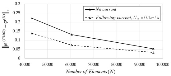
Figure 13. Convergence of the numerical solution obtained by the present FEM scheme in the case of waves with and without current scattered by a cylinder.

Next, in Figure 14, the convergence of the iterative scheme used to obtain a convergent solution in the case of waves and current scattered by a cylinder is presented. Results are presented for a coarse (N = 43,134 elements), a medium (N = 60,447 elements), a finer (N = 95,928 elements) and a fine grid (N = 171,860 elements). It can be observed that a convergent solution is achieved after 3–4 iterations. It is also noted here that the computation cost of the present 2D FEM scheme (using a standard configuration based on an i7, 2.6 GHz processor with 32 GB RAM), as compared to the 3D BEM of Section 2.2, is found to be less than 5% in terms of computer time and memory requirements.

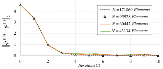
Figure 14. Convergence of the iterative scheme used to obtain a convergent solution by the present FEM scheme in the case of waves and current scattered by a cylinder. The iteration numbered 0 corresponds to the starting solution obtained without the current.

4.3. Resonances of Wave and Current Systems in the Case of a Line Array of Cylinders

Finally, we consider the case of normally incident waves in the tank scattered by a single row of vertical cylinders, seated on a flat horizontal bottom. Both the case of waves without current and the presence of a uniform following current are considered and results concerning the modulus and the real part of the field are presented in Figure 15 and Figure 16, respectively. Such configurations numerically simulate experiments in a flume for the investigation of resonance effects due to wave–current multiple cylindrical structure interactions.

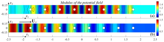
Figure 15. Modulus of the wave field in the 10 m long and 0.3 m wide waveguide of water depth h = 0.305 m, resulting from the interaction of an incident field of frequency $f=1.3\hspace{0.17em}\mathrm{H}\mathrm{z},$ with an array of eight cylinders (a) in the absence of currents and (b) in the presence of a steady following current corresponding to volumetric flow rate $Q=70.5\hspace{0.17em}{\mathrm{cm}}^{\mathrm{3}}/\mathrm{s}$.

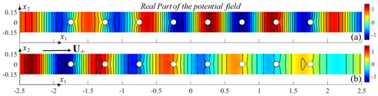
Figure 16. Real part of the wave field in the 10 m long and 0.3 m wide waveguide of water depth h = 0.305 m, resulting from the interaction of an incident field of frequency $f=1.3\hspace{0.17em}\mathrm{H}\mathrm{z}$, with an array of eight cylinders (a) in the absence of currents and (b) in the presence of a steady following current corresponding to volumetric flow rate $Q=70.5\hspace{0.17em}{\mathrm{cm}}^3/\mathrm{s}$.

In the examined test case, the vertical cylinder array is placed in a 10 m long and 0.3 m wide tank and a total number of eight equidistant cylinders positioned in line are considered in water depth $h=0.305\hspace{0.17em}\mathrm{m}$. The distance between centers of the cylinders is set to 0.5 m. Figure 15 and Figure 16 illustrate the modulus and the real part of the calculated wave field generated by the interaction of an incident wavefield of frequency $f=1.3\mathrm{Hz}$ with the above configuration of scatterers without current (Figure 15a and Figure 16a) and in the presence of current (Figure 15b and Figure 16b), respectively, as obtained by the present FEM. In the latter case, a following uniform current propagating at speed $U_{\infty }=0.077\hspace{0.17em}\mathrm{m}/\mathrm{s}$ corresponding to a volumetric flow rate in the numerical flume of $70.5\hspace{0.17em}{\mathrm{cm}}^3/\mathrm{s}$ is considered. As can be observed in these figures, the wave pattern, as well as the expected reflection and transmission characteristics, are substantially altered by the presence of the background current flow and scatterers.

The above configuration constitutes an interesting set-up to investigate limiting wavefield transformations, such as mode trapping, local amplitude amplification and resonance phenomena, and future research, also supported by a complementary experimental study, will be focused on this direction. Finally, extensions of the present method to treat effects by sheared currents (see, e.g., Belibassakis et al. [22]) are possible and will be considered in future work.

5. Conclusions

The problem of water wave scattering by arrays of vertical cylinders in the presence of background uniform currents in constant depth is considered and treated by a low-order hybrid 3D BEM, based on source and dipole distributions. The flow variables are decomposed, and the method is first used to calculate the steady perturbation field, generated by the uniform current. The resulting steady flow field is then used in order to formulate the wave diffraction problem and an iterative scheme is developed for the calculation of the interacting wave part, for monochromatic harmonic waves. As in the case of the steady flow problem, the corresponding wave and current scattering problem is numerically treated by 3D BEM in the frequency domain. Numerical results are presented and discussed, concerning the structure of both the steady and the time-dependent resulting fields, making the model suitable for applications in optimization studies. However, the above 3D model presents increased computational cost, which prevents its systematic use in the initial design stage, especially for complex configurations involving arrangements consisting of multiple cylindrical scatterers. For this purpose, for small current velocity, the problem can be approximately considered on the horizontal plane, modelled by the 2D Helmholtz equation with variable coefficients, which partially carries the effects of the variable current flow. The resulting 2D problem on the horizontal plane is numerically treated by a coupled BEM–FEM scheme, with substantially reduced computational cost. The effectiveness of the latter model is demonstrated, showing that the latter model can provide reasonable predictions and can be used for the preliminary study of the hydrodynamic characteristics of the considered configurations and support the design. Comparison against experimental data for further verification and calibration of the present simplified method is planned as the next step of research that will further support the study of the reflection/transmission characteristics and resonance phenomena in the case of complex configurations. Finally, extension of the present method to treat effects by vertically sheared currents interacting with waves and vertical cylindrical structures is also possible, and is planned to be studied in future work.

References

- Sulisz, W. Wave reflection and transmission at permeable breakwaters of arbitrary cross section. Coast. Eng. 1985, 9, 371–386. [Google Scholar] [CrossRef]
- Arnaud, G.; Rey, V.; Touboul, J.; Sous, D.; Molin, B.; Gouaud, F. Wave propagation through dense vertical cylinder arrays: Interference process and specific surface effects on damping. Appl. Ocean Res. 2017, 65, 229–337. [Google Scholar] [CrossRef]
- Belibassakis, K.A.; Gerostathis, T.P.; Athanassoulis, G.A. A coupled-mode model for water wave scattering by horizontal non-homogeneous current in general bottom topography. Appl. Ocean Res. 2011, 33, 384–397. [Google Scholar] [CrossRef]
- Belibassakis, K.; Arnaud, G.; Rey, V.; Touboul, J. Propagation and scattering of waves by dense arrays of impenetrable cylinders in a waveguide. Wave Motion 2018, 80, 1–19. [Google Scholar] [CrossRef]
- Molin, B.; Remy, F.; Arnaud, G.; Rey, V.; Touboul, J.; Sous, D. On the dispersion equation for linear waves traveling through or over dense arrays of vertical cylinders. Ocean Res. 2016, 61, 148–155. [Google Scholar] [CrossRef]
- Jamain, J.; Touboul, J.; Rey, V.; Belibassakis, K. Porosity Effects on the Dispersion Relation of Water Waves through Dense Array of Vertical Cylinders. J. Mar. Sci. Eng. 2020, 8, 960. [Google Scholar] [CrossRef]
- Li, Y.; Mei, C.C. Bragg scattering by a line array of small cylinders in a waveguide. Part 1. Linear aspects. J. Fluid Mech. 2007, 583, 161–187. [Google Scholar] [CrossRef]
- Linton, C.M.; Mclver, R. The scattering of water waves by an array of circular cylinders in a channel. J. Eng. Math. 1996, 30, 661–682. [Google Scholar] [CrossRef]
- Utsunomiya, T.; Eatock Taylor, R. Trapped modes around a row of circular cylinders in a channel. J. Fluid Mech. 1999, 386, 259–279. [Google Scholar] [CrossRef]
- Sumer, M.; Fredsoe, J. Hydrodynamics around Cylindrical Structures; Advanced Series on Ocean Engineering; World Scientific: Singapore, 1991; Volume 12. [Google Scholar]
- Ghadirian, A.; Vested, M.; Carstensen, S.; Christiensen, E.D.; Bredmose, H. Wave-current interaction effects on waves and their loads on a vertical cylinder. Coast. Eng. 2021, 165, 103832. [Google Scholar] [CrossRef]
- Thomas, G.P. Wave-current interactions: An experimental and numerical study. Part 1. Linear waves. J. Fluid Mech. 1981, 110, 457–474. [Google Scholar] [CrossRef]
- Belibassakis, K.A.; Athanassoulis, G.A.; Gerostathis, T. Directional wave spectrum transformation in the presence of strong depth and current inhomogeneities by means of coupled-mode model. Ocean Eng. 2014, 87, 84–96. [Google Scholar] [CrossRef]
- Noblesse, F. Alternative integral representations for the Green function of the theory of ship wave resistance. J. Eng. Math. 1981, 15, 241–265. [Google Scholar] [CrossRef]
- Katz, J.; Plotkin, A. Low Speed Aerodynamics; McGraw-Hill: New York, NY, USA, 2001. [Google Scholar]
- Belibassakis, K.A.; Kegkeroglou, A. A nonlinear BEM for the ship wave resistance. In Proceedings of the 18th International Congress of the International Maritime Association of the Mediterranean (IMAM2019), Varna, Bulgaria, 9–11 September 2019. [Google Scholar]
- Dawson, C.W. A practical computer method for solving ship-wave problems. In Proceedings of the 2nd International Conference on Numerical Ship Hydrodynamics, Los Angeles, CA, USA, 19–21 September 1977. [Google Scholar]
- Bonovas, M.; Belibassakis, K.; Rusu, E. Multi-DOF WEC Performance in Variable Bathymetry Regions Using a Hybrid 3D BEM and Optimization. Energies 2019, 12, 2108. [Google Scholar] [CrossRef]
- Kress, R. Linear Integral Equations; Springer: Berlin/Heidelberg, Germany, 1989. [Google Scholar]
- Karperaki, A.; Papathanasiou, T.K.; Belibassakis, K.A. An optimized parameter free PML FEM for wave scattering problems in the ocean and coastal environment. Ocean Eng. 2019, 179, 307–324. [Google Scholar] [CrossRef]
- Belibassakis, K.A.; Athanassoulis, G.A.; Gerostathis, T. A coupled-mode system for the refraction-diffraction of linear waves over steep three-dimensional topography. Appl. Ocean Res. 2001, 23, 319–336. [Google Scholar] [CrossRef]
- Belibassakis, K.; Touboul, J. A Nonlinear Coupled-Mode Model for Waves Propagating in Vertically Sheared Currents in Variable Bathymetry. Fluids 2019, 4, 61. [Google Scholar] [CrossRef]
Publisher’s Note: MDPI stays neutral with regard to jurisdictional claims in published maps and institutional affiliations. |
© 2022 by the authors. Licensee MDPI, Basel, Switzerland. This article is an open access article distributed under the terms and conditions of the Creative Commons Attribution (CC BY) license (https://creativecommons.org/licenses/by/4.0/).