Abstract
Active flow control with jet devices is a promising approach for vehicle aerodynamics control. In this work an extended computational study is performed comparing three different actuation strategies for active flow control around the square back Ahmed body at Reynolds number 500,000 (based on the vehicle height). Numerical simulations are run using a Large Eddy Simulation (LES) approach, well adapted to calculate the unsteady high Reynolds number flow control using periodic jet devices. computations are validated comparing to in-house experiments for uncontrolled and some controlled cases. The novelty of this investigation is mainly related to the in-depth study of the base flow and actuation approaches by an accurate LES method and their comparison to experiments. Here, several simulations are performed to estimate the effect of active controls on the flow topology and the drag reduction. Beside the continuous blowing jet, three periodic actuation techniques including periodic blowing and suction as well as the zero flux synthetic jet devices are explored. The slots are implemented discontinuously in order to achieve a better control efficiency linked to vortex generation. In this framework, spectral analyses on global aerodynamical quantities, rear pressure/drag coefficient behavior examination as well as wake structure investigations are performed in order to compare these jet actuations. As a result, shear layer variations are observed during the blowing phase, but the main flow topology change occurs with suction and synthetic jets. Rear back pressure is therefore substantially increased.
1. Introduction
Car manufacturers are dealing with the continuous challenging problem of improving energy performance of ground vehicles. Considering the flow behavior around most of the vehicle shapes, about 30% of global aerodynamical losses are due to the rear pressure forces [1]). Therefore, the design of efficient drag reduction strategies is a useful aerodynamical and environmental issue. However, this drag reduction should be obtained without constraints on the design, safety, comfort and habitability for the passengers. Thus, it is interesting to find flow control solutions, which will remove or make remote recirculation zones due to separation edges with active or passive devices [2]. Significant reduction of Cd can be obtained using passive techniques [3,4,5] and some of them are already used such as separated devices or deflectors localized in front of or behind the vehicle. Nevertheless, because of design and performance constraints, active flow control techniques contribute to an effective achievement of drag reduction. In this framework, various actuation approaches such as blowing and suction pulsed jets [6], synthetic jets [7], fluidic oscillators [8] or plasma actuators [9] could be employed to perform the active control. Moreover, it seems important to achieve a true understanding of the effect of these actuations on the flow topology and the shedding shear layer linked to the wall pressure and the drag reduction in order to select the best approach. There are several experimental investigations exploring the efficiency of oscillating jets; nevertheless, it appears there is a lack of data to study the modified near jet shear flow and its effect on the drag forces for turbulent flows around simplified vehicles. Therefore, computations seem necessary to achieve a better understanding of the local vortical structures generated by actuators.
In this work, numerical simulations on the flow behavior for three blowing pulsed, suction pulsed and synthetic jets are compared and analyzed on a square back Ahmed body that is commonly used as a simplified ground vehicle [10]. It is a three-dimensional bluff body moving in the vicinity of the ground generating a turbulent flow. Several separations appear along the body from the front to the back [11,12] and a slow and high wave length bi-stability occcurs [13,14]. The resulting recirculation zones contribute to a significant part of the Cd [15]. The flow for this geometry has been studied and extended to more realistic configurations in the framework of the underbody velocity effect [16] or the platoon of simplified trucks [17] and recently model reductions were performed to design learning strategies in order to predict flow topologies after geometrical modifications [18].
This coefficient changes strongly with the angle between the horizontal line and the rear window. For a square back Ahmed body (with a vertical rear window), corresponding to a simplified minivan or SUV vehicle, drag force reduction is a challenging objective for automotive industry due to the weak influence of the geometric parameters. The main objective, which is pursued generally, is the growth of the static pressure level in the wake with a well-settled active flow control device leading to a significant drag reduction. The control achievements can be verified by Cd, vorticity and velocity variations as well as wall static pressure measurements and simulations for square back simplified road vehicle setups [4,5,19,20,21,22]. Moreover, other studies have focused on the numerical analysis of devices installed in vehicles not only to reduce the drag, but also to increase the downforce [23,24]. They adopt Reynolds Average Navier-Stokes (RANS) model to analyze the effect of the Gurney flap for car racing application.
Here, the main focus is on the effect of the active control on the near wake topology and characteristics and their effect on the drag reduction for three different jet actuations. This computational study is performed using adapted Large Eddy Simulations with a particular emphasis on the signal type influence. Large Eddy Simulations are still considered as the most accurate computational approaches to simulate and control turbulent flows around such geometries [25,26]. The numerical method for the base flow is initially validated comparing to in house experiments before being generalized to controlled cases. Based on this, pulsed blowing jet, suction jet and synthetic jet impacts have been successively analyzed on global aerodynamical performances, shear layers, wake structures and finally on the rear pressure evolution. The novelty of this investigation is mainly related to the in-depth study of actuation approaches effect on the flow topology and body forces using a refined LES method and the comparison of uncontrolled and controlled case studies to in-house experiments for simplified road vehicle flows.
2. Numerical Model
2.1. Computational Set-Up
The geometry, illustrated in Figure 1, consists in a 0.7 scale model (compared to the original one) in a 4 m2 section wind tunnel. This later is a reproduction of the experimental wind tunnel as analyzed in [19,27]. In this framework the ground is not moving, therefore all the wall boundary conditions are no-slip with zero velocity vector on the boundaries. Moreover, the inlet boundary condition is set as a constant flow-rate leading to a 30 m/s velocity on the pitot tube located at 630 mm upstream of the nose of the Ahmed body and 1034 mm above the floor. Finally, the outlet boundary condition is fixed by the relative static pressure of zero. The actuation boundary conditions will be described in Section 3.2.
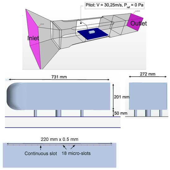
Figure 1.
Ahmed body and wind tunnel dimensions.
Kolmogorov in [28] proves that high Reynolds number flow involves a large range of turbulence scales. This system can’t be solved with a Direct Numerical Simulation (DNS) because it requires the resolution of Navier-Stokes equations for all turbulence scales. Thus, the spatial and temporal discretizations have to be precise enough to capture smallest structures. The Reynolds-Averaged Navier-Stokes approach gives low level of accuracy because separation and reattachment mechanisms require the resolution of a large range of turbulent scales while the method only solves turbulent statistical quantities. Large Eddy Simulation approach appears to be a better solution because smallest structures are managed by a subgrid-scale model. The remaining scales are computed solving Navier-Stokes equations in the same way as the . Consequently, the mesh does not have to be as fine as the DNS one. This is the compromise chosen in this work considering CPUs, time limitations and the level of accuracy required.
Many results in literature reach the same conclusion such as Krajnovic and Davidson in [29]. However, later in [30,31], advantages of hybrid approaches [32,33] such as Delayed Detached Eddy Simulation (DDES) [34], a zonal hybrid LES/RANS method or Partially Averaged Navier-Stokes method (PANS), a dynamic nodal hybrid DNS/RANS approach were discussed [31]. These methods have been developed quite recently and could have been an alternative to classical LES in order to save CPU time. However, despite its additional cost, the Large Eddy Simulation technique is still more accurate than hybrid methods as it avoids the RANS modelling for the boundary layer. The reduced scale configuration used in this paper allows to employ the LES approach with a reasonable cpu time. The LES approach used in this paper consists in the resolution of filtered Navier-Stokes equations for incompressible flows. Momentum and continuity equations are solved with a semi implicit second order numerical scheme in time and space implemented in a Galerkin least square finite element method. A refined unstructured mesh has been built in order to capture accurately all significant gradients in agreement to the local cut-off frequencies. Here, a rapid convergence thanks to a pre-conditioning iterative linear solver coupled to an iterative solver based on the Krylov method is enabled [35].
The filtered fields , denoted with a bar is defined as:
where is the filter test for the mesh grid cutoff and is the scalar field.
Thus Navier-Stokes equations become:
Here, and are filtered velocity components, the filtered pressure and the kinematic viscosity. With the strain rate tensor and the turbulent stress tensor defined as:
The resolution of these equations requires a closure relation for the turbulent stress tensor. A common method consists in doing an analogous of the molecular model using the Boussinesq hypothesis: the deviatoric part of the turbulent stress tensor is modeled as a function of the strain rate tensor:
Here, is the Kronecker Delta and is the turbulent viscosity. Then, a subgrid scale model is required to estimate the turbulent viscosity. In this work, it is computed with the Smagorinsky model:
with the cut-off local cell length size, the Van Driest damping function for no-slip wall boundary condition and the Smagorinsky constant.
This model is known to be highly robust but dissipative and a damping process using the closure relation for the turbulent stress tensor to compute the eddy viscosity in the core region with the dynamic Smagorinsky turbulence subgrid scale model is needed to reach a more accurate estimation of the dissipative scales correlated to the local level of turbulence [36,37]. Finally, filtered equations are solved using finite element approach with 2nd order numerical schemes.
According to Kolmogorov [28], for a Reynolds number of (based on the vehicle height), turbulence scale ranges from m ( with L the Ahmed body width) to wind tunnel height of 2 m. Furthermore, time scales ranges from 10 s () to the total averaging time required for this simulation. This later is about ten times the Ahmed body length over the reference velocity. Hence, 0.3 s averaging time is used. The cutoff wave number depends on discretization such as . With Large Eddy Simulation (LES) methods, discretization has to be fine enough to enable sufficient scale exact resolution. Pope [38] characterized the inertial/dissipative scale limitation assuming that maximum scale length structures are responsible for 90% of dissipation. In this case, it corresponds to 0.84 mm. These considerations lead to a mesh discretization compromise constituted of 120 million unstructured tetrahedral cells mesh illustrated in Figure 2 taking account of CPUs and memory resources [19]. Furthermore, the solver uses an implicit scheme letting to choose quite large time steps corresponding to a 2000 Hz frequency ( s). Simulations are performed on a 1.6 s physical time; as the convergence occurs after 0.6 s, 2000 snapshots are used to analyze the results.
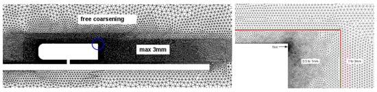
Figure 2.
Vertical transverse view of the mesh (left) with a focus on the rear back upper corner (right).
Wind tunnel conditions have been exactly reproduced numerically, so that the same effective blocking cross-section is applied as experiments. Computational limitations and data storage slightly reduces the mesh accuracy both for the Ahmed body’s wake shear layers and the entire wind tunnel boundary layer values. This leads to an effective cross-section error. To perform computation/experiment comparisons, a pitot probe measuring pressure value at a specific location is used as a reference point to be ensured about the cross-section integrity. Discrete numerical resolution and experimental datas are therefore comparable.
In addition, as expected with the solver wall function, the dimensionless wall distance displayed in Figure 3, is lower than 100 so that the boundary layer around the Ahmed body is correctly computed.
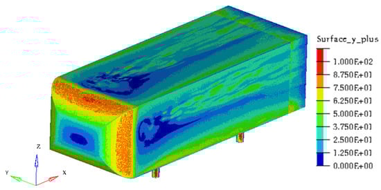
Figure 3.
plot on the Ahmed body wall surfaces.
2.2. Numerical Results Validation with Experiments
Three validation test cases, based on experimental data, have been used to estimate best numerical model performances and accuracy. The aim of these three test cases is to check the model ability to solve the flow topology as well as its ability to reproduce the actuator impact. Thus, the selected test simulations are: the reference case without any actuation, a low frequency pulsed jet actuation that deteriorates performances and a high frequency pulsed jet actuation that improves performances. Moreover, a grid convergence study from a previous research [19] enables to directly define mesh criteria for these computations as described in Section 2.1. To do so, drag coefficient is used as comparison criterion. It is defined as:
where and are the horizontally projected force and surface, the Pitôt velocity (see Figure 1) and the mass density. The reference surface corresponds to the projected frontal area.
Figure 4 compares the drag coefficients achieved by numerical simulations with the finest converged grid to in-house experimental data [19]. Drag coefficients have been measured experimentally for 14 consecutive pulsed jet frequencies from 10 to 500 Hz. Note that the frequency of ‘0 Hz’ refers to the uncontrolled flow. This figure also shows the simulated drag forces for three configurations without and with control (30 Hz and 400 Hz pulsed jets). The comparison of computations with experiments demonstrates a difference of for the uncontrolled case, for 30 Hz and for the 400 Hz pulsed jet controls. Thus, drag coefficients yield less than 1% error compared to the experiment for the reference case and the 400 Hz pulsed control.
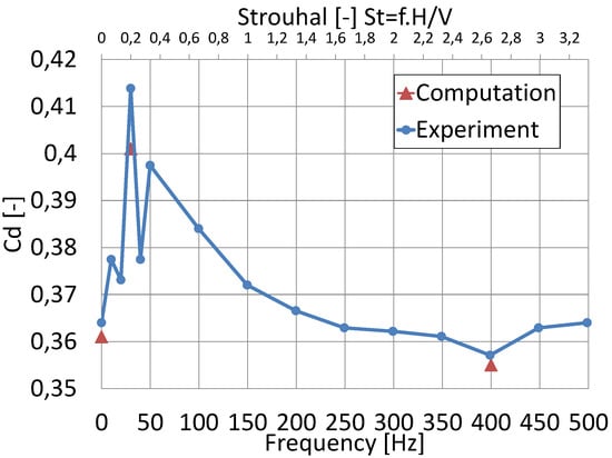
Figure 4.
Drag coefficient differences with respect to experimental reference case.
Furthermore, the flow topology in the back is correctly computed as shown in the rear back pressure map displayed in Figure 5. It denotes a similar flow topology between the numerical simulation and the experiment.
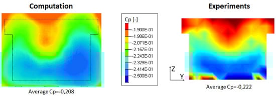
Figure 5.
Pressure coefficient distribution on the rear back end.
Both quantitative and topological validations prove that the present LES numerical simulations enable an accurate and realistic computation of the baseline and controlled flows around this configuration. Once the positive validations achieved, a deeper numerical study of actuator properties on the flow control efficiency is realized as follows.
3. Control Strategy Analysis
3.1. Description of the No-Controled Flow Topology
The system can be described by non dimensional characteristic coefficients. In addition to the drag coefficient Equation (6), there is the pressure coefficient computed using the rear surface integrated pressure defined as:
Slot actuation is characterized by the momentum coefficient defined as:
with the height of the slot ( mm), H the height of the Ahmed body rear wall and the magnitude of the jet velocity for all actuators. The actuation forcing frequency f is characterized by the Strouhal number:
The flow around the Ahmed body without any actuation has several characteristics. As shown in Figure 6, the sharp square back end leads to the boundary layer separation at each edge. It causes the development of shear layers corresponding to a high velocity gradient region.
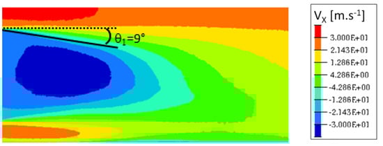
Figure 6.
Time-averaged velocity in the vertical transverse cut-plane (Oxz).
The sudden decrease of velocity generates a recirculation area with high pressure loss and high vorticity (Figure 7).
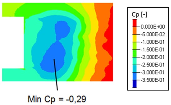
Figure 7.
Time-averaged pressure coefficient in the vertical transverse cut-plane (Oxz) at .
This pressure drop affects the rear back wall and increases significantly the overall drag forces (Figure 8).
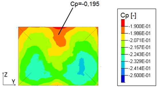
Figure 8.
Time-averaged pressure coefficient on the rear back end.
In this type of 3D unsteady and turbulent flow, the wake is alternatively governed by the different shear layers coming from each side of the Ahmed body. The balance between them results in a time average O-ring shape displayed on pressure iso-values of Figure 9. The slight unbalance observed in the vertical cut plane of Figure 7 is due to the ground effect.
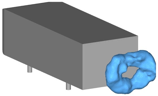
Figure 9.
O-ring structure shaped by time average pressure iso-contour.
The upstream flow feeding the recirculation area can be characterized by the lateral wall and the Ahmed body roof boundary layer. As shown in Figure 10, the lateral one is 15mm thick while the top one is 35 mm thick. Time average velocity isovalue of 30.3 m/s in the transverse cross section at x = H/10 displays a non uniform and non-symmetrical boundary layer shape around the vehicle. The turbulent kinetic energy () defined in Equation (10) and plotted in Figure 10, is the result of the flow separation:
with the flow fluctuation velocities for three dimensions.
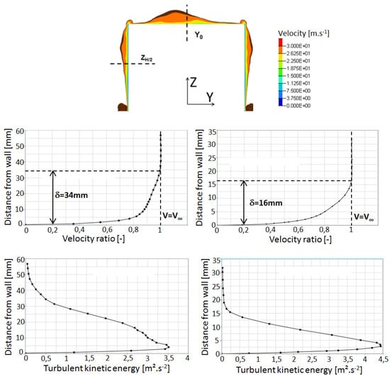
Figure 10.
(Top) Velocity profile under the boundary layer in the plane X = −H/10. (Middle) boundary layer thickness on the roof in the Y0 cut plane (left) and on the lateral bluff body at cut plane (right). (Bottom) turbulent kinetic energy profiles on the roof in the Y0 cut plane (left) and on the lateral bluff body at cut plane (right).
Figure 10 demonstrates that the maximum values for both profiles are at the distance of 5 mm from the wall. It is due to the front geometry bending radius as well as the road effect.
In Figure 11 the streamlines around the body display the local recirculation zone generated by the bending at .
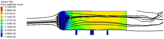
Figure 11.
Instantaneous streamlines around the Ahmed body with pressure distribution on the lateral wall.
Finally, several monitoring points in the wake vertical symmetry plane are selected to identify dominant flow frequencies and cross correlations as shown in Figure 12: The red point is in the area of lower pressure, the yellow dot captured the upper shear layer behavior and the green dot stand for the recirculation area. Cross spectra of these sensors with the sensor located at the black dot highlight some correlations and the related frequencies. This denotes a coherent mechanism with periodic behavior. For the sensor located in the upper shedding layer (yellow), the low frequency of 20 Hz (St = 0.13) corresponding to the near wake recirculating zone is strong and higher frequencies close to St = 0.6 (100 Hz) fitting to the shear layer fluctuations interaction with the recirculating area are also measured. For the point in the lower part of the time averaged minimum pressure area (red), the frequency of 20 Hz (St = 0.13) is emerging too. We can suppose that this frequency denotes a vertical alternating activity related to a double recirculation zone. Another frequency of 26 Hz (St = 0.17) is dominative in this location as well as for the dot located downstream in the wake (green); this represents the shedding frequency of structures expelled outside the recirculating area in the wake. This behavior is described in [29].
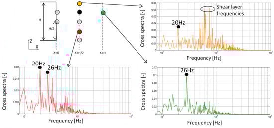
Figure 12.
Wake structure spectral analysis.
This reference simulation helped to identify the outlines of the flow topology.
3.2. Design of Experiment and Sensitivity Analysis for Flow Control
A large design of experiment has been realized based on the variation of several parameters:
- Actuator slot geometry: one continuous slot or 18 discontinous slots as shown in Figure 1. The control device is introduced on the upper edge of the back wall in order to better interact with the roof separation vortex area (best location of active flow control actuators [39]).
- Jet angles: 90 degrees to 30 degrees from rear back wall;
- Velocity magnitude: 30 m/s to 150 m/s;
- Signal type: constant jet vs pulsed suction jet vs pulsed blowing jet vs synthetic jet;
- Actuator frequency: 30 to 750 Hz.
Results of this design of experiment have allowed to approach an optimal point considering the cost of the flow control actuators: Fisrt of all, geometrically continuous jets generates quite poor control compared to the discontinuous 18 slots case. Moreover, every slot dimension is mm. The test case with 18 slots blowing at 90 degrees and 75 m/s is chosen as the best configuration because of its high drag reduction performance. This design of experiment also demonstrates the superiority of the 400 Hz forcing frequency of the synthetic jet actuator as shown in Figure 13 and Table 1.
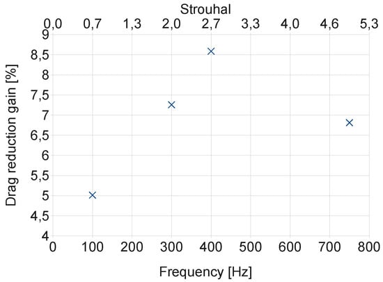
Figure 13.
Drag reduction computed as a function of the forcing frequency with synthetic jets, versus the uncontrolled flow. We can notice a gain of at the forcing frequency of 400 Hz, corresponding to .

Table 1.
Time averaged quantities.
Therefore, the following parameters are chosen for the actuator study: Geometrical discontinuous slots, 90 degrees jets angle, 75 m/s jets velocity and 400 Hz actuators forcing frequency that correspond to the actuation boundary conditions.
The design of experiment returns an interesting influence of the signal type on the final drag reduction. The Figure 14 shows a comparison of mean simulation results from the point of view of drag reduction and energy consumption, between 4 different signals: constant blowing, pulsed suction, pulsed blowing and synthetic jets. Indeed, the drag reduction gain obtained with synthetic jet is higher that the one obtained for test cases with pulsed and uniform jets leading to the best flow efficiency. The second best solution is the suction pulsed jet at the same frequency.
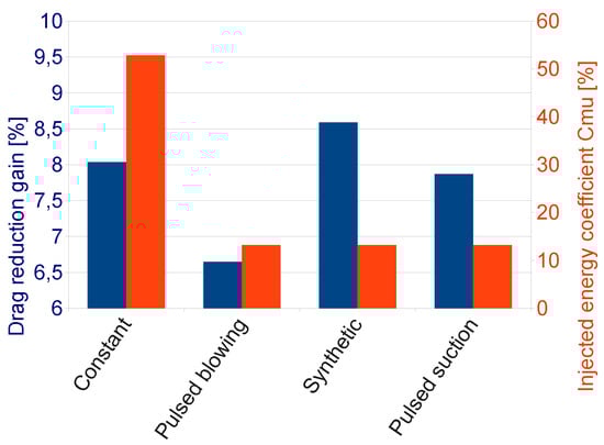
Figure 14.
Mean drag reduction values and jet flow efficiency for different signal types. The best performance is achieved using synthetic jets.
The constant blowing jet appears to be less efficient considering that there is the same amount of drag reduction than other actuation types with a higher energy consumption as seen in Figure 14. Therefore, this case will be discarded for the following study and we will only focus on pulsed and synthetic actuators in the next section.
A more precise computational analysis of the flow topology is performed in the following in order to understand the jet impact according to the signal type. It has been realized with best parameters identified previously.
3.3. Actuation Type Influence on the Flow Topology and Behavior
An appropriate choice of the actuator type for flow control is an important issue for engineers. Here, a detailed comparison between pulsed (blowing or suction) and synthetic jets is presented and their influence on the flow topology and drag reduction is studied. As explained in the Section 3.2, the control device is implemented at the top edge of the back wall and contains 18 5 × 0.5 mm separated slots Figure 1.
- Time averaged maincharacteristics
First, time averaged quantities show that the synthetic jet enhances sensibly the control performance better than both pulsed blowing and suction jets as shown in Table 1, even if the blowing jet has a better drag reduction than the suction one.
In Table 1, the pressure minimum values and their distance in the (XZ, Y = 0) cut plane from the back wall for the upper and lower recirculation areas are presented (see also Figures 24–26). Minima pressure centers are lower for the suction jet meaning that the wake negative pressure is less influence by the actuation. Their positions are also closer to the rear back wall and the reerence case. The blowing phase has more influence on the resulting wake pressure loss. However pulsed suction jet still gives better drag reduction than pulsed blowing jet. This property is related to the near wake recirculation asymetry and will be explained later.
On the other hand, the wake minimum pressure is located in the lower part of the recirculation bubble for the blowing pulsed jet actuator as well as the reference case without control. This is not the case anymore for pulsed suction and synthetic actuators meaning that the near wake equilibrium changes.
This proves that the injected flow does not only push back the mean torus but also modifies its balance.
- Shearlayer
Instantaneous vorticity and pressure observations in vertical Y0 cut plane during several steps of the actuation cycle offer an understanding of the local jet’s impact. Figure 15 and Figure 16 show the vorticity and pressure fields in the vicinity of the pulsed blowing and suction actuators for 4 time cycles (Figure 17). The low pressures are increased and the cycle achieves its optimum value at step 4 of the cycle. The comparison with the synthetic jet effect (Figure 18) demonstrates that the synthetic jet has a more continuous effect on the eddy structures than other actuations and the pressure field is dramatically influenced.
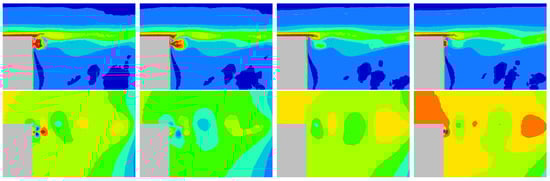
Figure 15.
Snapshots of the upper shear layer for blowing pulsed jet in the Y0 cut plane from step 1 (left) to step 4 (right): (Top) Vorticity, (Bottom) Pressure.
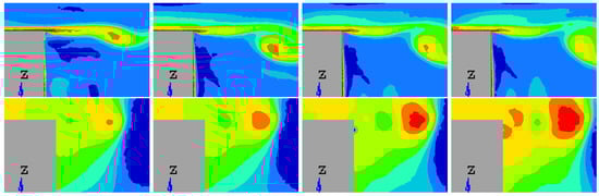
Figure 16.
Snapshots of the upper shear layer for suction jet in the Y0 cut plane from step 1 (left) to step 4 (right): (Top) Vorticity, (bottom) Pressure.
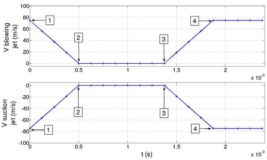
Figure 17.
Blowing pulsed jet (Top) and Suction jet (Bottom) signal cycle.
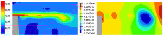
Figure 18.
Snapshots of the upper shear layer for synthetic jet in the Y0 cut plane: (Left) Vorticity, (Right) Pressure.
The periodicity of actuators are sources of regular spaced pressure variations impacting downstream pressure loss. Suction phases action on the shear layer is less clear. But pressure variations are increased.
These features are also visible with synthetic actuations.
Time average fields in the XZ cut plane across a middle slot give more informations on the global jet impact.
The average flow for blowing pulsed jet displays a spread velocity gradient locally in the vicinity of the actuation as shown in Figure 19.
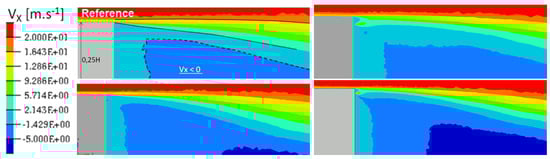
Figure 19.
Time-averaged x-velocity (m/s) for reference case (Top left), pulsed jet (Top right), suction jet (Bottom left) and synthetic jet (Bottom right).
There is also more velocity fluctuations in this area as shown in the turbulent kinetic energy fields (Figure 20 and Figure 21), defined by the Equation (10). In Figure 20, the turbulent kinetic energy is presented in the whole computational wake and with a zoom on the upper near wake in Figure 21. The blowing pulsed actuation tends to feed the mixing layer and increases the interaction between the upper flow and the jet flow. Hence turbulence intensity in the horizontal boundary layer before the top edge is strongly reduced. The pulsed blowing jets decrease drastically the TKE in the shear layers and in the vicinity of the back wall.
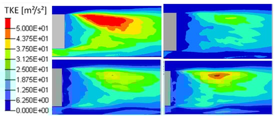
Figure 20.
Turbulent kinetic energy in the Y0 cut plane: reference case (Top left), pulsed jet (Top right), suction jet (Bottom left) and synthetic jet (Bottom right).
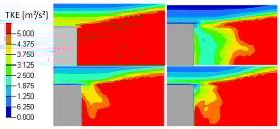
Figure 21.
Turbulent kinetic energy in the Y0 cut plane: reference case (Top left), pulsed jet (Top right), suction jet (Bottom left) and synthetic jet (Bottom right).
On the other hand, suction seems to induce higher velocity fluctuations below the actuator inflow and the recirculation area is moved closer to the back wall.
The turbulence level is increased in downstream leading to a change of the shear layer vorticity shape (Figure 22). Finally, for synthetic jets, we recognize a similarity between the blowing jet for the actuation area but the recirculation zone shift toward the back wall is more similar to the suction jet.
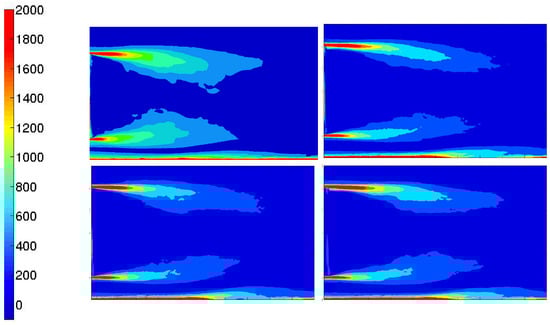
Figure 22.
Time-averaged vorticity (s) for reference case (Top left), pulsed jet (Top right), suction jet (Bottom left) and synthetic jet (Bottom right).
The synthetic jet also decreases the recirculation zone turbulent kinetic energy compared to the reference case even if its effect is less drastic than the pulsed jet.
The recirculation area is actually longer with a small deviation towards the inner recirculation bubble as illustrated by the time averaged vorticity fields in Figure 22. This is in agreement with pressure minima positions. Suction jets avoid drastically the stretching of the shear layers far from the rear back wall and the ratio between the top and the bottom shear layer is reduced. Thus, the top shear flow has a greater effect on the recirculation area using the only suction control. This can explain why the upper pressure minimum is larger than the lower pressure minimum for suction and synthetic jets.
- Recirculation bubble
Time averaged pressure field for blowing pulsed jet test case generates a homogeneous O-ring in the wake (Figure 23). The torus is the result of the fluid flow coming from above and below the Ahmed body that alternatively feed the recirculation zone. Therefore, global flow topology is similar to the reference case (Figure 24) except that the torus pressure level is higher with −0.26 pressure coefficient instead of −0.29 for the uncontrolled case. The suction pulsed jet (Figure 25), on the other hand, leads to an unstructured O-ring shape. If in the previous case, the mean flow was completely organized around the torus pressure structure, in the suction case, more separated areas with proper pressure entities take shape in the near wake. The area located downstream of the jet inflow is the result of pressure variations caused by actuators. Contrary to the pulsed blowing jet, pressure variations don’t smooth together but remain separated from the downstream pressure torus. This zone also explains the curvature deviation of the velocity isolines in Figure 19.
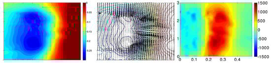
Figure 23.
Time-averaged pressure coefficient (Left), adverse pressure gradient and isolines (Centre) and x-component of pressure gradient (Right) for pulsed jet in the Y0 cut plane.
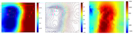
Figure 24.
Time-averaged pressure coefficient (Left), adverse pressure gradient and isolines (Centre) and x-component of pressure gradient (Right) for reference case in the Y0 cut plane.
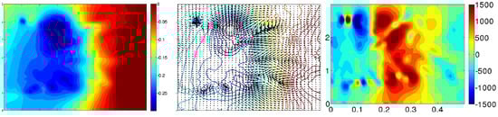
Figure 25.
Time-averaged pressure coefficient (Left), adverse pressure gradient (Centre) and x-component of pressure gradient (Right) for suction jet in the Y0 cut plane.
The outbreak of other pressure loss areas for pulsed jets in the vicinity of the lower shear layer proves that the balance between the upper recirculation and the lower one is different from the reference case. This is particularly noticeable on the x component of the pressure gradient (Figure 25). In fact, wake pressure gradient is notably increased with suction jets compared to pressure gradient with blowing pulsed jets that is almost uniform in the area between extrema points and the wall. Nevertheless, despite the shear layer’s shortening, as well as the shift of the pressure minima values and positions, recirculation bubble still has less impact on the wall when suction jets are used. The synthetic control simulation (Figure 26) also leads a structured torus but it is pushed back to downstream. In this case, there is no separated pressure point. All pressure variations are blent into a unique torus. The remaining pressure variations distort pressure isolines in a peak but does not impact on the torus position. The instantaneous pressure variations is therefore more pronounced than the ones generated by the blowing pulsed jet and their interactions with the recirculation structure is increased compared to the suction jet simulation. So they don’t prevent the equilibrium between the upper and the lower part. There is also a uniform pressure gradient between the torus and the rear back wall but the recirculation zone is larger than the pulsed jet case.
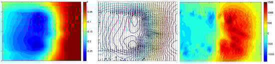
Figure 26.
Time-averaged pressure coefficient (Left), adverse pressure gradient (Centre) and x-component of pressure gradient (Right) for synthetic jet in the Y0 cut plane.
Pressure coefficient standard deviation, illustrated in Figure 27, corresponds to the pressure fluctuation magnitude around the time averaged field function. It gives a better understanding of the resulting time averaged flow behaviour. Suction and synthetic jets generate higher pressure variations in the vicinity of the jet inflow. In addition, even if the recirculation bubble acts as a low pass filter, as shown in Figure 28, suction and synthetic actuators display a higher propagation of pressure variations. Moreover, the lower part of the recirculation also exhibits higher pressure variations. Actuation has therefore more influence on the global recirculation area.
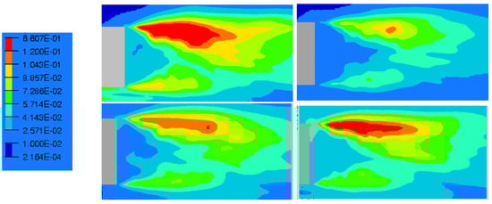
Figure 27.
RMS values of pressure in the Y0 cut plane: reference case (Top left), pulsed jet (Top right), suction jet (Bottom left) and synthetic jet (Bottom right).

Figure 28.
Power spectral density for a probe at x = H/2 from the rear back end for pulsed jet (left), suction jet (centre) and synthetic jet (right).
- Rear pressure
Finally, time averaged rear pressure map is the inprint of the recirculation wake structure for all test cases. Some low frequency transverse oscillations lead to a mean asymmetry in the synthetic test case changing fundamentally the flow topology as seen in Figure 29.
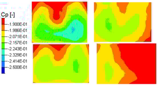
Figure 29.
Mean pressure coefficient on the rear back end in the Y0 cut plane: reference case (Top left), pulsed jet (Top right), suction jet (Bottom left) and synthetic jet (Bottom right).
Rear back spectral quantities are mainly governed by the actuator forcing frequency (Figure 30). However, pressure phase averaging, illustrated in Figure 31, displays significant specificities depending on the signal type. It is particularly sensitive to the jet velocity variations. Indeed, it evolves approximately in the same way as the jet flow oscillations especially with suction and synthetic jets.
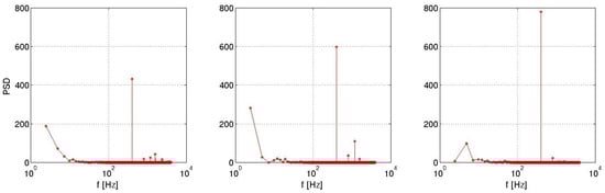
Figure 30.
Power spectral density of the pressure coefficient integrated on the rear back end.
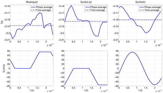
Figure 31.
Phase average rear pressure (top) and velocity jet (bottom).
This may be correlated to the influence of spatial pressure variations on the recirculation evolution. These variations are reinforced with suction and synthetic signals but the blowing phase of synthetic actuator tends to increase their interactions with the global pressure loss.
Pressure coefficient standard deviation on the rear back, Figure 32, is almost zero for pulsed jet except in the vicinity of jet inflow. Thus the blowing flow doesn’t impact the overall pressure distribution. Suction and synthetic jets allow an efficient control of the overall pressure map. That is why there is such a strong correlation between the jet velocity and the integrated pressure.
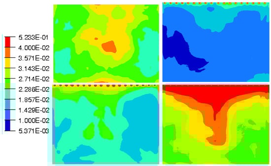
Figure 32.
RMS values of pressure coefficient on the rear back end: reference case (Top left), pulsed jet (Top right), suction jet (Bottom left) and synthetic jet (Bottom right).
However, correlation between the jet velocity and the pressure coefficient for pulsed jet is only visible locally for the probe 1 located close to the roof edge slots (Figure 33). Indeed, the pulsed frequency is only visible for the probe 1 by the power spectral densities (PSD) illustrated in Figure 34. Figure 34 and Figure 35 illustrate that for the pulsed jet, pressure coefficient of the probe 1 evolves in a same way as the suction jet sensor. Other sensors are subjected to different pressure fluctuations that deteriorate the periodic pattern. For the suction jet simulation, all sensors behave in a same way similar to the integrated signal. Finally, all probes for the synthetic jet computation are sinusoidal signals in quadrature phase with respect to the jet signal as seen in Figure 36.
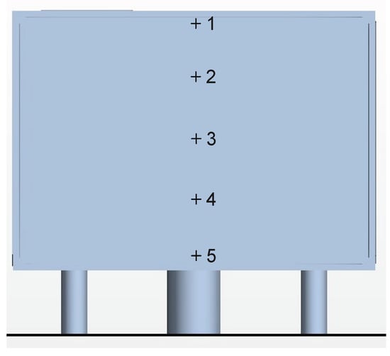
Figure 33.
Probe (sensor) locations.
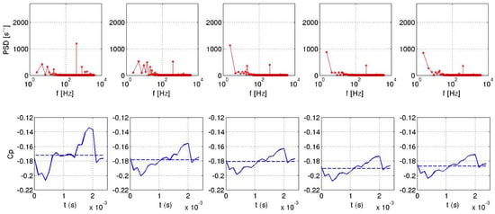
Figure 34.
Power spectral density for probes 1 (left) to 5 (right) for pulsed jet.
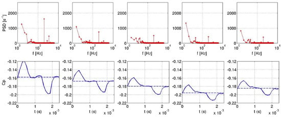
Figure 35.
Power spectral density for probes 1 (left) to 5 (right) for suction jet.
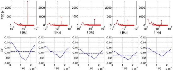
Figure 36.
Power spectral density for probes 1 (left) to 5 (right) for synthetic jet (right).
It appears that synthetic jets generate very slightly damped oscillations in the wake flow which can explain the good result of the drag reduction for this control technique. This phenomenon is observed investigating the fluctuations captured by all sensors located in Figure 33 at the middle of the body.
4. Conclusions
In this paper, a LES solver used for the flow control was compared to the square back Ahmed body experimental results such as wall pressure on rear wall as well as measured drag coefficient values and validated achieving a suitable accuracy. Then a wide range of simulations were performed for three different active controls with pulsed, suction and synthetic jets in order to explore their effect on the flow topology and drag reduction. The numerical model used for the LES computations was able to capture the flow modifications of the shear layer for the different actuation jet devices. The selected time step was appropriate to predict the vortical structures convection with low numerical diffusion.
These computations highlighted natural and actuated flow frequencies present in the shear layers and in the near wake. The optimum forced frequencies inducted by the pulsed periodic inlet flow conditions in the upper shear layer decreased the turbulent kinetic energy in the interaction zone between the shear layer and the wake and consequently increased the minimum of pressure in the recirculation zone. Indeed, the shear layer spreading in the vicinity of blowing pulsed jets were observed.
Due to the mixed results obtained initially with blowing pulsed jet actuation, periodic inlet flow conditions were extended to suction and synthetic jet boundary conditions. Simulation results obtained with these new configurations showed the interest of the suction phase in order to increase the pressure fluctuations in the recirculation area close to the upper shear layer, already present with pulsed jets at the same forced frequencies. Then, the combined pulse/suction strategy, revealed the efficiency of the synthetic jet boundary conditions applied on the horizontal discontinuous slots enabling to reduce drag values of the mockup up to 8% at 400 Hz. The main reason of the synthetic jet efficiency seems to be linked to the two alternating phases between pulsing and suction which distinctly separate vortex structures created by the actuation and advect them into the shear layer.
Even if pulsed jet actuators are easy to manipulate on a test bench, autonomy of synthetic jet could be a great advantage in order to implement this family of actuators on a ground vehicle. Moreover, active control with synthetic jets generates the best drag reduction without any air supply.
In conclusion, this study permitted to confirm the accuracy and stability of these unsteady simulations involving the LES method to investigate the efficiency of different active control solutions dealing with periodic jets. To go further, closed-loop control with machine learning can be applied to design optimal periodic actuator boundary conditions in particular for synthetic jet devices. This real-time control could potentially provide a solution to minimize dynamically the jet momentum and the drag coefficient, taking into account the system’s state and the flow dynamics history.
Author Contributions
Conceptualization, S.E., P.G. and I.M.; methodology, S.E., P.G. and I.M.; software, S.E.; validation, S.E., P.G.; formal analysis, S.E., P.G. and I.M.; investigation, S.E., P.G. and I.M.; resources. S.E., P.G. and I.M.; data curation, S.E., P.G. and I.M.; writing—original draft preparation, S.E., P.G. and I.M.; writing—review and editing, P.G. and I.M.; visualization, S.E.; supervision, S.E. and I.M.; project administration, P.G. and I.M.; funding acquisition, P.G. and I.M. All authors have read and agreed to the published version of the manuscript.
Funding
This paper was partially founded by the AMIES (Agence pour les Mathématiques en Interaction avec l’Entreprise) with Plastic Omnium.
Acknowledgments
This work was initially funded by AMIES with Plastic Omnium collaboration. The authors are grateful to ALTAIR for providing the AcuSolve license for simulations.
Conflicts of Interest
The authors declare no conflict of interest.
References
- Barnard, R. Road Vehicle Aerodynamic Design: An Introduction; Longman: Harlow, UK, 1996. [Google Scholar]
- Fiedler, H.E.; Fernholz, H.H. On management and control of turbulent shear flows. Prog. Aerosp. Sci. 1990, 27, 305–387. [Google Scholar] [CrossRef]
- Roshko, A.; Koening, K. Interaction effects on the drag of bluff bodies in tandem. In Aerodynamic Drag Mechanisms of Bluff Bodies and Road Vehicles; Springer: Boston, MA, USA, 1978; pp. 253–286. [Google Scholar] [CrossRef]
- Bruneau, C.H.; Gillieron, P.; Mortazavi, I. Passive control around the two-dimensional square back Ahmed body using porous devices. J. Fluids Eng. 2008, 130, 061101. [Google Scholar] [CrossRef]
- Khalighi, B.; Chen, K.H.; Iccarino, I.G. Unsteady Aerodynamic Flow Investigation Around a Simplified Square-Back Road Vehicle With Drag Reduction Devices. J. Fluids Eng. 2012, 134, 061101. [Google Scholar] [CrossRef]
- Aider, J.L.; Joseph, P.; Ruiz, T.; Gilotte, P.; Eulalie, Y.; Edouard, C.; Amandolese, X. Active flow control using pulsed micro- jets on a full-scale production car. Int. J. Flow Control 2014, 6, 1–20. [Google Scholar] [CrossRef]
- Mohseni, K.; Mittal, R. Synthetic Jets: Fundamentals and Applications; CRC Press: Boca Raton, FL, USA, 2014. [Google Scholar]
- Schmidt, H.; Woszidlo, R.; Nayeri, C.; Paschereit, C. Separation control with fluidic oscillators in water. Exp. Fluids 2017, 58, 135. [Google Scholar] [CrossRef]
- Karimi, S.; Zargar, A.; Mani, M.; Hemmati, A. The Effect of Single Dielectric Barrier Discharge Actuators in Reducing Drag on an Ahmed Body. Fluids 2020, 5, 244. [Google Scholar] [CrossRef]
- Ahmed, S.R.; Ramm, G.; Faltin, G. Some salient features of time-averaged ground vehicle wake. SAE Tech. Pap. Ser. 1984, 93, 840222–840402. Available online: https://www.jstor.org/stable/44434262 (accessed on 10 December 2021).
- Minguez, M.; Brun, C.; Pasquetti, R.; Serre, E. Experimental and high-order LES analysis of the flow in near-wall region of a square cylinder. Int. J. Heat Fluid Flow 2011, 32, 558–566. [Google Scholar] [CrossRef]
- Roumeas, M.; Gilliéron, P.; Kourta, A. Separated Flows Around the Rear Window of a Simplified Car Geometry. J. Fluids Eng. 2008, 130, 021101. [Google Scholar] [CrossRef]
- Bonnavion, G.; Cadot, O. Unstable wake dynamics of rectangular flat-backed bluff bodies with inclination and ground proximity. J. Fluid Mech. 2018, 854, 196–232. [Google Scholar] [CrossRef]
- Podvin, B.; Pellerin, S.; Fraigneau, Y.; Bonnavion, G.; Cadot, O. Low-order modelling of the wake dynamics of an Ahmed body. J. Fluid Mech. 2021, 927, R6. [Google Scholar] [CrossRef]
- Roumeas, M.; Gilliéron, P.; Kourta, A. Analysis and control of the near-wake flow over a square-back geometry. Comput. Fluids 2009, 38, 60–70. [Google Scholar] [CrossRef]
- Castelain, T.; Michard, M.; Szmigiel, M.; Chacaton, D.; Juvé, D. Identification of flow classes in the wake of a simplified truck model depending on the underbody velocity. J. Wind Eng. Ind. Aerodyn. 2018, 175, 352–363. [Google Scholar] [CrossRef]
- Bruneau, C.H.; Khadra, K.; Mortazavi, I. Flow analysis of square-back simplified vehicles in platoon. Int. J. Heat Fluid Flow 2017, 66, 43–59. [Google Scholar] [CrossRef]
- Zancanaro, M.; Mrosek, M.; Stabile, G.; Othmer, C.; Rozza, G. Hybrid Neural Network Reduced Order Modelling for Turbulent Flows with Geometric Parameters. Fluids 2021, 6, 296. [Google Scholar] [CrossRef]
- Eulalie, Y.; Gilotte, P.; Mortazavi, I. Numerical study of flow control strategies for a simplified square back ground vehicle. Fluid Dyn. Res. 2017, 49, 035502. [Google Scholar] [CrossRef]
- Cooper, K.R. The effect of front-edge rounding and rear-edge shapping on the aerodynamic drag of bluff vehicles in ground proximity. SAE Pap. 1985, 94, 727–757. Available online: https://www.sae.org/publications/technical-papers/content/850288/ (accessed on 10 December 2021).
- Bruneau, C.H.; Creusé, E.; Depeyras, D.; Gillieron, P.; Mortazavi, I. Active procedures to control the flow past the Ahmed body with a 25 degree rear window. Int. J. Aerodyn. 2011, 1, 299–317. [Google Scholar] [CrossRef]
- Schmidt, H.; Woszidlo, R.; Nayeri, C.; Paschereit, C. The effect of flow control on the wake dynamics of a rectangular bluff body in ground proximity. Exp. Fluids 2018, 59, 107. [Google Scholar] [CrossRef]
- Basso, M.; Cravero, C.; Marsano, D. Aerodynamic Effect of the Gurney Flap on the Front Wing of a F1 Car and Flow Interactions with Car Components. Energies 2021, 14, 2059. [Google Scholar] [CrossRef]
- Fernandez-Gamiz, U.; Gomez-Mármol, M.; Chacón-Rebollo, T. Computational Modeling of Gurney Flaps and Microtabs by POD Method. Energies 2018, 11, 2091. [Google Scholar] [CrossRef] [Green Version]
- Maulenkul, S.; Yerzhanov, K.; Kabidollayev, A.; Kamalov, B.; Batay, S.; Zhao, Y.; Wei, D. An Arbitrary Hybrid Turbulence Modeling Approach for Efficient and Accurate Automotive Aerodynamic Analysis and Design Optimization. Fluids 2021, 6, 407. [Google Scholar] [CrossRef]
- Krajnović, S. Large Eddy Simulation Exploration of Passive Flow Control Around an Ahmed Body. J. Fluids Eng. 2014, 136, 121103. [Google Scholar] [CrossRef] [Green Version]
- Eulalie, Y. Etude Aérodynamique et Contrôle de la Traînée sur un corps de Ahmed Culot Droit. Ph.D. Thesis, Université de Bordeaux, Talence, France, 2014. [Google Scholar]
- Kolmogorov, A.N. The local structure of turbulence in incompressible viscous fluid for very large Reynolds numbers. R. Soc. Lond. Proc. Ser. A 1991, 434, 9–13. [Google Scholar] [CrossRef]
- Krajnovic, S.; Davidson, L. Large Eddy Simulation of the Flow around Simplified Car Model; SAE Paper No. 2004-01-0227; SAE International: Detroit, MI, USA, 2004. [Google Scholar]
- Krajnovic, S.; Minelli, G.; Basara, B. Partially-Averaged Navier-Stokes Simulations of Bluff Body Flows. In Proceedings of the ICCFD8 International Conference on Computational Fluid Dynamics, Chengdu, China, 14–16 July 2014. [Google Scholar]
- Mirzaei, M.; Krajnović, S.; Basara, B. Partially-Averaged Navier–Stokes simulations of flows around two different Ahmed bodies. Comput. Fluids 2015, 117, 273–286. [Google Scholar] [CrossRef]
- Ekman, P.; Wieser, D.; Virdung, T.; Karlsson, M. Assessment of hybrid RANS-LES methods for accurate automotive aerodynamic simulations. J. Wind Eng. Ind. Aerodyn. 2020, 206, 104301. [Google Scholar] [CrossRef]
- Guilmineau, E.; Deng, G.; Leroyer, A.; Queutey, P.; Visonneau, M.; Wackers, J. Assessment of hybrid RANS-LES formulations for flow simulation around the Ahmed body. Comput. Fluids 2018, 176, 302–319. [Google Scholar] [CrossRef]
- Delassaux, F.; Mortazavi, I.; Itam, E.; Herbert, V.; Ribes, C. Sensitivity analysis of hybrid methods for the flow around the ahmed body with application to passive control with rounded edges. Comput. Fluids 2021, 214, 104757. [Google Scholar] [CrossRef]
- Corson, D.; Jaiman, R.; Shakib, F. Industrial application of RANS modelling: Capabilities and needs. Int. J. Comput. Fluid Dyn. 2009, 23, 337–347. [Google Scholar] [CrossRef]
- Germano, M.; Piomelli, U.; Moin, P.; Cabot, W.H. A Dynamic Subgrid-Scale Eddy Viscosity Model. Phys. Fluids A Fluid Dyn. 1991, 3, 1760–1769. [Google Scholar] [CrossRef] [Green Version]
- Cintolesi, C.; Mémin, E. Stochastic Modelling of Turbulent Flows for Numerical Simulations. Fluids 2020, 5, 108. [Google Scholar] [CrossRef]
- Pope, S.B. Turbulent Flows; Cambridge University Press: Cambridge, UK, 2000. [Google Scholar] [CrossRef]
- Bruneau, C.H.; Creuse, E.; Depeyras, D.; Gilleron, P.; Mortazav, I. Coupling active and passive techniques to control the flow past the square back Ahmed body. Comput. Fluids 2010, 39, 1875–1892. [Google Scholar] [CrossRef]
Publisher’s Note: MDPI stays neutral with regard to jurisdictional claims in published maps and institutional affiliations. |
© 2022 by the authors. Licensee MDPI, Basel, Switzerland. This article is an open access article distributed under the terms and conditions of the Creative Commons Attribution (CC BY) license (https://creativecommons.org/licenses/by/4.0/).