Abstract
In the framework of innovative aerodynamics, active airfoils can be developed and exploited based on the integration of shape memory metal alloys (SMAs), allowing for surface adaptation, i.e., shape changes in response to operative thermal inputs, depending on the desired aerodynamic behavior. The purpose of thermally activated shape-changing (TASC) airfoils’ improved capabilities is to offer benefits in terms of aircraft performance and fuel consumption rate. TASC airfoil design hinges upon three intertwined and nonlinear phenomena, namely the solid–fluid–thermal interactions. In this paper, in order to approach the definition of appropriate design parameters, the space of operating variables is explored for the first time by devising a finite element method simulation encompassing the equations of structural motion, energy, and turbulent Reynolds-averaged Navier–Stokes. Such a fully coupled model is then tested by implementing a sensitivity analysis for a preliminary design of a TASC/NACA airfoil. Temperature and velocity distributions are presented and discussed, including new metrics leading to aerodynamic lift calculations. When the efficiency is computed as the lift-to-drag ratio, it is found to vary nonlinearly in the 0–45 range, with the activating power feed in the 0–1000 W range.
1. Introduction
With aerodynamics being the major aspect influencing body design, as Pern and Jacob [1] first speculated, the application and exercise of discrete adaptive surfaces can represent a viable solution to reach these goals. In this framework, there is a growing interest in morphing wing technologies that are reaching a high technological readiness level [2,3]. Morphing wings are studied in the aviation industry to improve aircraft performance by adapting their shapes to flight conditions such as the take-off, landing, and cruise phases. Improved performance and reduced fuel consumption represent two important goals that must nowadays be taken into account in aerodynamic design. The progress in aviation research is paving the way to also introduce morphing structure technologies in the automotive industry [4], whereas their application is mainly addressed to high-performance vehicles, though not only with the aim of reducing drag and optimizing lift (downforce).
Conceptual design, prototype fabrication, and the evaluation of shape-changing wings were classified by Sofla et al. [5]. Computational research dealing with active-load-control airfoil appendices can be relevant to this task [6]. In the past, such airfoils were realized by requiring mechanical actuators providing the specific degree of freedom, with the weight and structural performance affecting their efficiency and cost. The development of active airfoils, capable of improving aerodynamics performance by autonomous shape-changing and continuous adaptation to specific inputs while keeping added weight at a minimum, is therefore a worthy area of investigation.
It is well known that shape memory alloys (SMAs) are optimal materials for adaptive surfaces [3,7,8]. SMAs exist in two crystalline structures: martensite is present at lower temperatures, and austenite is present at higher temperatures. The reason for the particular structural behavior of an SMA-integrated airfoil is the transition between the two phases: the temperature increase due to Joule heating causes the beginning of the transition, inducing a force that produces a desired geometry variation suitable for the chosen operating condition [9]. Generally, unlike most metals, SMAs contract in length when heated but will maintain the same absolute volume. An embedding matrix provides that every other material property requirement is satisfied.
One such material is nitinol (NiTi) [3], for which a major stakeholder, NASA, has been long aware of its purposeful properties [10]: as an example, NiTi can be used in deployable vortex generators [11]. The design and realization of this kind of dynamic SMA system relies on structural considerations [12]. Figure 1 reports on one such thermally activated shape-changing (TASC) airfoil case by employing SMAs.
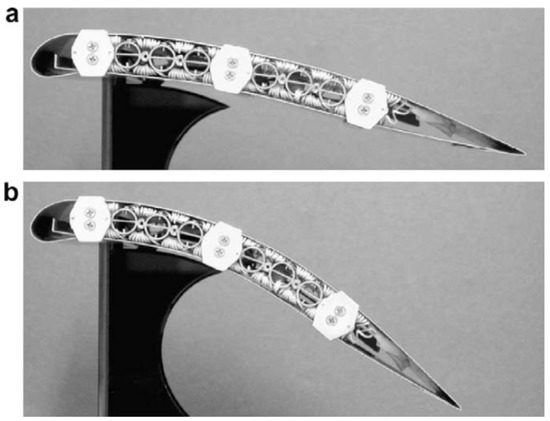
Figure 1.
Chord-wise bending of an adaptive airfoil, achieved by the heating of SMA strips in an antagonistic configuration: (a) initial and (b) adapted shape [13].
Clearly, modelling and numerical simulation are important tools to improve the performance prediction of morphing structures. Structural, aerodynamic and thermal effects have often been studied in decoupled environments; structural and thermal analyses are relatively simple to approach by finite element modeling (FEM) methods, while aerodynamics can be approached by panel potential methods or computational fluid dynamics (CFD) computations. Due to the strong interactions between structural, thermal and aerodynamic effects, a reliable approach should consider these effects in a coupled environment but the complex mechanisms involved make this approach very difficult; indeed, there is lack of coupled analyses in the literature.
Recently, a comprehensive literature review on the possible SMA shape-change applications has been offered by Sellitto and Riccio [14]. However, a strong fluid-structure interaction (FSI) is expected when adaptive airfoils are immersed in a flow field. A thorough review on FSI was provided by Hou, Wang and Layton [15], while Ismail et al. [16] and MacPhee and Beyene [17] studied the shape changes of wings and wind turbines. Machairas et al. [18] analyzed FSI by a FEM, but TASC effects were not considered.
As TASC airfoils are locally subject to internal and discrete heating, it is clear that their adaptive feature is driven by heat transfer. This problem is properly attacked by solving the momentum and heat transfer simultaneously in both the solid (airfoil) and fluid (flowing air) phases. This approach allows no empirical assumptions to be made. As alluded to earlier, structural design must be coupled to thermal study [19], which is strictly correlated to fluid dynamics interactions. Thermal FSI is a multidisciplinary area of scientific investigation of formidable difficulty even without the thermal problem [20].
A first model of a fully coupled TASC plate has been recently presented by Caccavale et al. [21], but with no inference on airfoil morphing. In this paper, this analysis is extended for the first time, with reference to said solid–fluid–thermal interactions, to a more suitable shape for practical applications, i.e., a common aerodynamic airfoil. A fully-coupled simulation is proposed encompassing the variable space that emerges from the equations set. A sensitivity analysis of the intertwined and nonlinear phenomena set is implemented, and a new metric is proposed to help preliminarilyy design thermally activated aerodynamics appendices, with special references to aerodynamic lift and efficiency. Power feeds up to 1 kW and nominal air velocity up to 30 m/s (108 km/h) are assessed. The efficiency, when computed as the lift-to-drag ratio, is found to increase slowly for power feeds higher than 600 W. The present preliminary model and associated results lay the foundations for further development in the field of TASC airfoils.
2. Materials and Methods
2.1. Assumptions
The lift build-up needed in aerodynamic operations is obtained by a suitable airfoil shape morphing; thus, a strong interaction between boundary layer development and continuous shape change was obtained and analyzed. A NACA 0012 airfoil with mm chord length was immersed in a horizontal flow of standard air in a turbulent regime (fluid phase f, Figure 2). In the present study, the Reynolds number employed (based on the relative free-stream air velocity and airfoil chord) was such that a turbulent regime was ensured in the control volume at hand, as described next. In any studied configuration, the transfer phenomena were studied in a steady state.
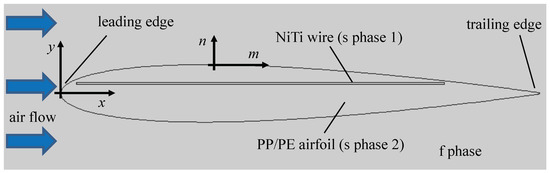
Figure 2.
Detail of the control volume under scrutiny, with indication of solid and fluid phases. Global (centered on the leading edge) and local coordinates are also reported.
A 0.6 mm dia. wire in NiTi (solid phase s1) was embedded length-wise in the airfoil, which was made of a PP–PE copolymer (solid phase s2). An appropriate electric current was applied to the wire in order to modify its structural condition and attain the desired shape change. The two solid phases are isotropic and with perfect structure matching. The properties of solid phase s1 change according to the the SMA’s behavior, while solid phase 2 has constant properties. Inelasticity and hysteresis effects in structural modeling were not taken into account in the present study (only a one-time transformation from the martensite phase to the austenite phase is considered).
2.2. Sequence of Phenomena Coupling
In shape-changing by means of SMA structural variation, when acquired in static condition (i.e., in still air without FSI inference), heat transfer due to the applied electric current has a one-way relationship to structural mechanics, as discussed by Caccavale et al. [21]. However, in TASC airfoil design, heat convection occurs on the airfoil’s surface due to exposure to the given velocity air flow, and lift and drag results when FSI is supplemented in the analysis. Thus, fluid and structural mechanics are directly two-way related, and they are also indirectly one-way related through the occurrence of heat transfer: the solid displacement is balanced by the force exerted by the fluid on the airfoil, whereas heat generation dictates shape change, but in turn is depleted by heat convection at the exposed surface.
2.3. Governing Equations
With reference to the control volume represented in Figure 2, and employing a tensor representation, the governing equations for the 3 mechanisms at stake are as follows.
2.3.1. Solid Mechanics
The equation of motion in the steady-state assumption reads as
with representing the identity matrix, representing the solid displacement vector, representing the stress tensor, and representing the volumetric force vector.
Hooke’s law relates the stress and strain tensors in the absence of contributions from initial and viscoelastic stresses:
where the double-dot tensor product is employed. Here, the fourth-order elasticity tensor is defined in terms of Young’s modulus and Poisson’s ratio [22]:
while the strain tensor may be written in terms of :
2.3.2. Fluid Flow
The Reynolds-averaged Navier–Stokes (RANS) equations can be written, in a regime of pure forced convection, as:
with representing the averaged fluid velocity vector, representing the viscous stress tensor in the boundary layer, p representing the averaged pressure, and and with the usual meanings. The present model is based on the low-Reynolds closure model [23], bringing the relationship for the turbulent dynamic viscosity . This turbulent paradigm can model heat fluxes with good accuracy in conjunction with boundary layer flows, providing for a very accurate description of the flow field, as it supplements with damping functions for turbulence, thus performing a realistic limiting behavior. For the sake of brevity, the equations for the transfer of turbulent kinetic energy, k, and turbulent dissipation rate, , are left unreported here.
2.3.3. Energy
Thermal energy is transferred macroscopically in the fluid phase and microscopically in the solid phase s (comprising both s1 and s2).
- Fluid phase f:
- Solid phase s:with representing the temperature of the s phase, representing the averaged temperature of the f phase (see Figure 2), representing the nominal power feed to the SMA wire, representing the power related to latent heat due to the martensite-to-austenite transformation, representing the volume of the s phase 1, and and with the usual meanings.
2.4. Boundary Conditions and Couplings
- SMA wire, or solid phase s1: prescribed power determining the volumetric force :While the SMA behavior specifying the function in Equation (9) is detailed in [22,24] (referring to the common Lagoudas formulation for SMA), the SMA properties employed are reported in Table 1.
 Table 1. Solid-phase properties.
 - Embedding airfoil, or solid phase s2: the solid phase is structurally free everywhere, with the exception of the leading edge, which has a fixed constraint:Additionally, the volumetric force in the embedding airfoil is given by the inherent external force or aerodynamic force (due to FSI effects) supplied to , the volume of the s phase 2 (see Figure 2):implying that .
- Air–free-stream boundary: the control volume of fluid phase is very long along x and wide along y with respect to the airfoil length and thickness, respectively (see Figure 2). Therefore, the air is issued to the control volume with prescribed conditionsalong with a 15% free-stream turbulence intensity exercised for the application at stake.
- Solid–fluid interface: thermal continuity and no-slip, requiringrespectively, along with the usual conditions for the chosen turbulence paradigm, again left unreported here for the sake of brevity. The thermal continuity condition allows to solve the temperature field simultaneously in both the solid and fluid phases in a conjugate fashion, i.e., with no need to impose a convective heat flux (based on a simplistic heat transfer coefficient at the solid–fluid interface).
- Outflow boundaries: outlet conditions requiringalong with the usual conditions for the chosen turbulence paradigm, again left unreported here for the sake of brevity.
- Thermal FSI coupling: coupling between solid mechanics and fluid mechanics meshes is imposed through the mutual geometry change, whose numerical treatment is presented next. The structural and fluid problems are defined and solved in their respective phases only, whereas the thermal problem is solved in both phases.
2.5. Numerical Method
A FEM commercial software, COMSOL Multiphysics [25], was employed to solve the system of Equations (1)–(8) with its boundary conditions in the control volume outlined in Figure 2. The overall size of the computational domain was 30 × l and along x and y, respectively, allowing for non-reflecting boundary conditions at the far field. A pressure-based RANS solver was employed with the turbulence closure model.
First, a multifrontal massively parallel sparse direct solver (MUMPS) was employed for wall distance initialization, with a relative tolerance of ; then, again, the MUMPS was invoked for stress, whereas a parallel direct sparse solver with a relative tolerance of was used in a segregated fashion with row preordering and multithreaded forward and backward solving to ensure computational stability and robustness, first for velocity and pressure and finally for temperature.
A grid dependency study was performed, exercising up to 4 grid sizes. In Figure 3, the computed drag coefficient (to be referred to later) for is plotted against mesh size, showing a fair convergence. Thus, grid level 2 was adopted in all computations. This grid also scored a positive check on and (invariance at the 4th and 3rd meaningful digit, respectively). In the f phase, the final grid featured a boundary layer (b.l.) of 2 levels with a minimum edge of 3 × m and a stretching factor of 1.2, up to a final edge of m, for a total of almost triangular cells plus more than 300 quadrilateral cells in the b.l. In the s phase, this grid had almost 2400 and 330 triangular cells in the s1 and s2 phases, respectively. This grid, reported in Figure 4, allowed for properly resolving the velocity and temperature gradients in the b.l. along the s–f interface.
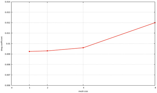
Figure 3.
Grid dependency study: computed drag coefficients versus mesh size levels.
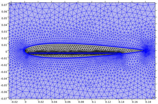
Figure 4.
Detail of the employed grid. Blue and black colors are used to emphasize the different phases in the control volume.
2.6. FSI Treatment
The geometrical changes of both solid and fluid phases were achieved by adopting an arbitrary Lagrangian–Eulerian (ALE) moving mesh formulation [25]. The spatial frame was allowed to be separated from the material frame according to a frame transformation driven by to the computed structural displacement, . The structural deformation of the material frame (solved for in a Lagrangian meaning) drove the variation of locations of mesh nodes in the spatial frame. The force computed in the fluid flow (solved for in an Eulerian meaning) contributed to driving the structural force, inducing deformation, . The mesh deformation was smoothed to ensure the stability of the numerical solver with high-quality mesh elements by means of the Yeoh model [26].
2.7. Overall Computational Remarks
The following libraries were exploited in the software employed [25]: solid mechanics with the SMA option, turbulent flow, and heat transfer (in both fluids and solids), including the link to said SMA option. All physics invoked were selected such that their computations were inherently fully coupled and joined with the above ALE formulation.
The Reynolds number based on chord length was typically around , which is a “transitional” Reynolds number for airfoils. In the present case, a 15% free-stream turbulence intensity was assumed, such that turbulent conditions were ensured.
The model was verified for a classical (un-morphed and no power feed) configuration against the lift and drag coefficients, as reported later in Section 3.2.
3. Results and Discussion
3.1. Explored Variables Space and Auxiliary Definitions
A sensitivity analysis was carried out by varying the nominal power feed to the SMA wire, , and the nominal free-stream air velocity, , to explore the TASC operation with reference to Equations (1)–(8) and the related boundary conditions from Equations (9)–(14). The pressure was atmospheric, and the free-stream air temperature was 300 K.
The aerodynamic force was computed by the integration of the stresses acting in the boundary layer formed on the airfoil surface in the f phase:
where S is the airfoil exposed surface, is the versor normal to S (see Figure 2), and represents the viscous stress tensor in the boundary layer, as in Equation (6). To calculate the aerodynamics performance for the TASC airfoil, the resulting lift and drag can be computed by projecting along the n and m directions, respectively.
The local skin friction coefficient is computed as:
while the lift and drag coefficients are, respectively, defined by:
with l being the airfoil chord. Finally, to propose a metric leading to preliminary lift calculations on thermally activated appendices, the lift-to-drag ratio (aerodynamic efficiency) is reported as:
3.2. Comparison with the Available Literature for an Airfoil with No Power Feed
The coefficients defined in Equation (17) are relevant to the evaluation of the soundness of the calculations performed. The computed drag at returns a drag coefficient equal to 0.0093 (93 drag counts), while the lift coefficient varies from 0 to 0.65. The computed values of and are in good agreement with experiments and numerical calculations in the literature on NACA 0012 airfoils at the given Reynolds number range in fully turbulent flow [27,28] considering the increasing curvature of the airfoil while increasing .
3.3. Temperature Distributions
The solution for temperature in the airfoil and in the surrounding air is presented next, which is useful to help comply with material specificationss with a changing power feed at the SMA wire. This model may then be applied to verify that the maximum temperature falls within the requirement for the given airfoil to be tested. To this end, five temperature maps are reported in Figure 5 with varying : the maximum temperature in the solid phase is found to be around 500 K in the top frame case, when W. In the same frame, the thermal discharge or spout resulting from the conjugate solution of Equations (7) and (8) is also indicated.
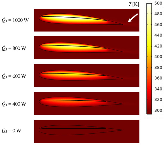
Figure 5.
Maps of temperature T at a free-stream air velocity m/s for five cases of power feed , from 0 to 1000 W, with indication of the thermal discharge past the trailing edge of the airfoil.
Figure 5 shows that thermal non-uniformity plays a role in preventing the desired operation and ensures uniform SMA activation: indeed, the SMA wire ends appear to be immersed in a matrix standing up to 100 K colder than its midsection. Therefore, this model could be used to address the compliancy of the assembly in the design phase.
3.4. Air Velocity Distributions, Lift and Drag
The solution for the air velocity is reported in Figure 6, where five velocity maps are reported with varying : the maximum velocity is found to be around 35 m/s over the suction side in the top frame case when W.
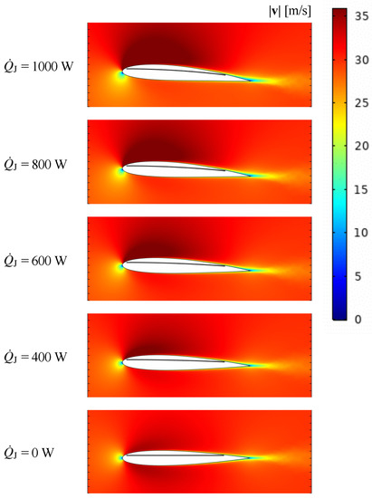
Figure 6.
Qualitative maps of air velocity magnitude at a free-stream air velocity m/s for cases of power feed from 0 to 1000 W.
It is interesting to note that, due to the FSI effect, the TASC airfoil would be slightly flattened out, i.e., the deflection would have been greater if the airfoil was not immersed in a airflow, with the related pressure difference inducing a force directed to straighten the airfoil in its otherwise static shape.
Furthermore, the lift and drag offered by the airfoil are reported by Figure 7 for the entire range of the nominal power feed, whereas the aerodynamic efficiency is reported by Figure 8. An almost linear lift increase with power feed is obtained in Figure 7, left: this is obviously due to the increased airfoil curvature. Differently than the lift force, drag force has a non-linear increase in Figure 7, right, growing slowly at low power feeds, while a non-linear increase of form drag is evidenced at higher power feeds due to flow separation at the trailing edge zone. This effect can also be appreciated in Figure 8, where the aerodynamic efficiency is plotted against power feed. At high power feeds, there is an evident decrease in efficiency growth rate that must be taken into account in the design phase of SMA-operated airfoils.
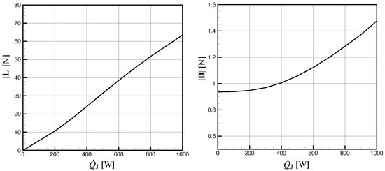
Figure 7.
Lift (left) and drag (right) forces for the operational range of the nominal power feed .
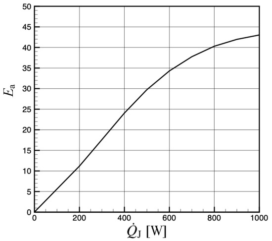
Figure 8.
Aerodynamic efficiency for the operational range of the nominal power feed .
It is worth remarking that the aerodynamic efficiency is somewhat greater than the one computed for a flat plate [21], whereas the present computations are more reliable for practical aerodynamic applications.
4. Conclusions
A fully coupled steady-state model has been proposed and solved with a sensitivity analysis to the combined solid–fluid–thermal interactions that featured the shape-change of an airfoil immersed in a turbulent flow and cast with a SMA wire. The interdependent nature of the phenomena has been discussed, stemming from the insertion of the thermal problem (due to the thermal activation of the SMA-cast airfoil) in an otherwise pure FSI framework. A complex set of partial differential equations was set up with due generality to facilitate applications for other geometries, and the role of the SMA material has been enforced by exploiting a Lagoudas formulation. Finally, an arbitrary Lagrangian–Eulerian moving mesh formulation has been employed to catch the peculiarities of the FSI problem.
Temperature and velocity distributions were described and discussed depending on the driving parameters, namely the free-stream velocity and the power feed to the SMA composite. The model showed correct predictions for the classical airfoil configuration. The velocity distribution could be calculated by taking into consideration the changing shape with the adopted steady-state solution procedure: the air would reach up to 35 m/s over the airfoil’s suction side in the most deflected geometry (maximum power feed at the SMA wire). Then, the solution of temperature was treated in a conjugate fashion. Thermal nonuniformity, with temperatures topping up to 500 K in the airfoil core for the maximum tested power feed of 1 kW, has been found that could hinder the desired shape change and, in turn, the aerodynamic function, and this should be addressed in the design phase. Airfoil inflection and lift and drag values (with the efficiency varying nonlinearly in the 0–45 range) were then calculated, showing the purposeful nature of the TASC simulator as a preliminary design tool.
Author Contributions
Conceptualization, G.R.; methodology and software, P.C.; formal analysis, B.M. and G.R.; data curation, G.R.; writing—original draft preparation, G.R.; writing—review and editing, B.M. and G.R.; visualization, P.C. and G.R.; supervision and funding acquisition, M.B. and G.R. All authors have read and agreed to the published version of the manuscript.
Funding
This research was funded by European Union co-financing—FSC, PON Research and Innovation 2014-2020 ARS01_00882 “Active Responsive Intelligent Aerodynamics”.
Conflicts of Interest
The authors declare no conflict of interest.
Abbreviations
The following abbreviations are used in this manuscript:
| ALE | Arbitrary Lagrangian–Eulerian |
| FEM | Finite element method |
| FSI | Fluid–structure interaction |
| NACA | National Advisory Committee for Aeronautics |
| PP–PE | polypropylene–polyethylene |
| SMA | Shape memory alloy |
| TASC | Thermally activated shape-changing |
References
- Pern, N.J.; Jacob, J.D. Aerodynamic flow control using shape adaptive surfaces. In Proceedings of the 1999 ASME Design Engineering Technical Conferences; ASME: New York, NY, USA, 1999; pp. 1–8. [Google Scholar]
- Li, D.; Zhao, S.; Da Ronch, A.; Xiang, J.; Drofelnik, J.; Li, Y.; Zhang, L.; Wu, Y.; Kintscher, M.; Monner, H.P.; et al. A review of modelling and analysis of morphing wings. Prog. Aerosp. Sci. 2018, 100, 46–62. [Google Scholar] [CrossRef]
- Barbarino, S.; Flores, E.S.; Ajaj, R.M.; Dayyani, I.; Friswell, M.I. A review on shape memory alloys with applications to morphing aircraft. Smart Mater. Struct. 2014, 23, 063001. [Google Scholar] [CrossRef]
- Daynes, S.; Weaver, P.M. Review of shape-morphing automobile structures: Concepts and outlook. Proc. Inst. Mech. Eng. Part D J. Automob. Eng. 2013, 227, 1603–1622. [Google Scholar] [CrossRef]
- Sofla, A.Y.N.; Meguid, S.A.; Tan, K.T.; Yeo, W.K. Shape morphing of aircraft wing: Status and challenges. Mater. Des. 2010, 31, 1284–1292. [Google Scholar] [CrossRef]
- Mayda, E.A.; Van Dam, C.P.; Nakafuji, D. Computational investigation of finite width microtabs for aerodynamic load control. In Proceedings of the 43rd AIAA Aerospace Sciences Meeting and Exhibit, Reno, NV, USA, 10–13 January 2005; pp. 1185–1198. [Google Scholar]
- Bashir, M.; Lee, C.F.; Rajendran, P. Shape memory materials and their applications in aircraft morphing: An introspective study. J. Eng. Appl. Sci. 2017, 12, 50–56. [Google Scholar]
- Bashir, M.; Rajendran, P.; Sharma, C.; Smrutiranjan, D. Investigation of smart material actuators & aerodynamic optimization of morphing wing. Mater. Today Proc. 2018, 5, 21069–21075. [Google Scholar]
- Kumar, P.K.; Lagoudas, D.C. Introduction to shape memory alloys. In Shape Memory Alloys; Springer: Berlin/Heidelberg, Germany, 2008; pp. 1–51. [Google Scholar]
- Cross, W.B.; Kariotis, A.H.; Stimler, F.J. Nitinol Characterization Study; Technical report; NASA: Pasadena, CA, USA, 1969.
- Memory Metals are Shaping the Evolution of Aviation. Available online: www.nasa.gov/feature/glenn/2019/memory-metalsare-shaping-the-evolution-of-aviation (accessed on 15 December 2022).
- Scalet, G.; Niccoli, F.; Garion, C.; Chiggiato, P.; Maletta, C.; Auricchio, F. A three-dimensional phenomenological model for shape memory alloys including two-way shape memory effect and plasticity. Mech. Mater. 2019, 136, 103085. [Google Scholar] [CrossRef]
- Elzey, D.M.; Sofla, A.Y.N.; Wadley, H.N.G. A shape memory-based multifunctional structural actuator panel. Int. J. Solids Struct. 2005, 42, 1943–1955. [Google Scholar] [CrossRef]
- Sellitto, A.; Riccio, A. Overview and future advanced engineering applications for morphing surfaces by shape memory alloy materials. Materials 2019, 12, 708. [Google Scholar] [CrossRef] [PubMed]
- Hou, G.; Wang, J.; Layton, A. Numerical methods for fluid-structure interaction – a review. Commun. Comput. Phys. 2012, 12, 337–377. [Google Scholar] [CrossRef]
- Ismail, N.I.; Zulkifli, A.H.; Talib, R.J.; Zaini, H.; Yusoff, H. Drag performance of twist morphing MAV wing. In Proceedings of the MATEC Web of Conferences; EDP Sciences: Les Ulis, France, 2016; Volume 82, p. 01004. [Google Scholar]
- MacPhee, D.W.; Beyene, A. Fluid–structure interaction analysis of a morphing vertical axis wind turbine. J. Fluids Struct. 2016, 60, 143–159. [Google Scholar] [CrossRef]
- Machairas, T.; Kontogiannis, A.; Karakalas, A.; Solomou, A.; Riziotis, V.; Saravanos, D. Robust fluid-structure interaction analysis of an adaptive airfoil using shape memory alloy actuators. Smart Mater. Struct. 2018, 27, 105035. [Google Scholar] [CrossRef]
- Barbarino, S. SMAs in Commercial Codes. In Shape Memory Alloy Engineering; Elsevier: Amsterdam, The Netherlands, 2015; pp. 193–212. [Google Scholar]
- Scholten, W.; Hartl, D.J. An Uncoupled Method for Fluid-Structure Interaction Analysis with Application to Aerostructural Design. In Proceedings of the AIAA Scitech 2020 Forum, Orlando, FL, USA, 6–10 January 2020; p. 1635. [Google Scholar]
- Caccavale, P.; Mele, B.; De Bonis, M.V.; Ruocco, G. Analysis of thermally activated fluid-structure interaction for a morphing plate immersed in turbulent flow. Int. J. Heat Mass Transf. 2022, 194, 123081. [Google Scholar] [CrossRef]
- Machado, L.G.; Lagoudas, D.C. Thermomechanical constitutive modeling of SMAs. In Shape Memory Alloys; Springer: Berlin/Heidelberg, Germany, 2008; pp. 121–187. [Google Scholar]
- Abe, K.; Kondoh, T.; Nagano, Y. A new turbulence model for predicting fluid flow and heat transfer in separating and reattaching flows – I. Flow field calculations. Int. J. Heat Mass Transf. 1994, 37, 139–151. [Google Scholar] [CrossRef]
- Lagoudas, D.C. Shape Memory Alloys: Modeling and Engineering Applications; Springer: Berlin/Heidelberg, Germany, 2008. [Google Scholar]
- COMSOL Multiphysics v.5.6; COMSOL AB: Stockholm, Sweden, 2020.
- Renaud, C.; Cros, J.M.; Feng, Z.Q.; Yang, B. The Yeoh model applied to the modeling of large deformation contact/impact problems. Int. J. Impact Eng. 2009, 36, 659–666. [Google Scholar] [CrossRef]
- Abbott, I.H.; Von Doenhoff, A.E. Theory of Wing Sections: Including a Summary of Airfoil Data; Courier Corporation: North Chelmsford, MA, USA, 2012. [Google Scholar]
- Gregory, N.; O’reilly, C.L. Low-Speed Aerodynamic Characteristics of NACA 0012 Aerofoil Section, including the Effects of Upper-Surface Roughness Simulating Hoar Frost; Number 3726; Ministry of Defence, Aeronautical Research Council: London, UK, 1970.


Disclaimer/Publisher’s Note: The statements, opinions and data contained in all publications are solely those of the individual author(s) and contributor(s) and not of MDPI and/or the editor(s). MDPI and/or the editor(s) disclaim responsibility for any injury to people or property resulting from any ideas, methods, instructions or products referred to in the content. |
© 2023 by the authors. Licensee MDPI, Basel, Switzerland. This article is an open access article distributed under the terms and conditions of the Creative Commons Attribution (CC BY) license (https://creativecommons.org/licenses/by/4.0/).