Abstract
Highway buses are used in a wide range of commuting services and in the tourist industry. The demand for highway bus transportation has dramatically increased in the recent post-pandemic world, and airborne transmission risks may increase alongside the demand for highway buses, owing to a higher passenger density in bus cabins. We developed a numerical prediction method for the spatial distribution of airborne transmission risks inside bus cabins. For a computational fluid dynamics analyses, targeting two types of bus cabins, sophisticated geometries of bus cabins with realistic heating, ventilation, and air-conditioning were reproduced. The passengers in bus cabins were reproduced using computer-simulated persons. Airflow, heat, and moisture transfer analysis were conducted based on computational fluid dynamics, to predict the microclimate around passengers and the interaction between the cabin climate and passengers. Finally, droplet dispersion analysis using the Eulerian–Lagrangian method and an investigation of the spatial distribution of infection/spread risks, assuming SARS-CoV-2 infection, were performed. Through parametric analyses of passive and individual countermeasures to reduce airborne infection risks, the effectiveness of countermeasures for airborne infection was discussed. Partition installation as a passive countermeasure had an impact on the human microclimate, which decreased infection risks. The individual countermeasure, mask-wearing, almost completely prevented airborne infection.
1. Introduction
Public transportation is an essential part of modern society and plays an important role in social activities. Among the various forms of public transportation, highway buses are widely used in a wide range of commuting services and in the tourist industry. The demand for these dramatically decreased in the pandemic period, and has increased in the recent post-pandemic period. The highway bus cabin has a high passenger density, and its use for long trips in a closed space increases airborne transmission risks even though the filtering of airborne pathogens by the heating, ventilation, and air-conditioning (HVAC) systems can contribute to reducing airborne infection risks [1]. It is concerning that the rebound of demand for commuting in reduced transportation services in the transition period to post-pandemic results in higher passenger densities. Therefore, it is necessary to estimate airborne transmission risks inside highway bus cabins to control airborne infection risks among passengers. Ultimately, this contributes to human wellness and reduces social costs.
In highway bus cabins, the HVAC system plays an important role in maintaining good air quality because natural ventilation is not available due to there being closed windows. Moreover, considering heat sources including solar radiation and human heat generation in bus cabins, the operation of the HVAC system is essential for the thermal comfort of passengers. Owing to these circumstances, non-uniform environmental factors including airflow patterns and the thermal environment are ever-present in bus cabins, which HVAC systems are installed to alleviate [2]. This is also an important health risk factor in bus cabins because there are various factors which cause health risks, such as chemical contaminants, carbon dioxide (CO2) accumulation, and airborne transmission in pandemic situations, and ventilation rates in bus cabins are often limited owing to the energy consumption of the HVAC system. This implies that the bus cabin environment has to be optimized, considering the environmental factors in the bus cabin.
Many researchers have used field measurements and numerical analysis to estimate the quality of the environment in bus cabins. The air quality in the bus cabin and its relationship with environmental conditions inside and outside of the bus cabin have been investigated [3,4,5,6,7]. It was revealed that bus cabin air quality can be significantly affected by outdoor air contaminants including particulate matter (PM) and gas phase contaminants from traffic. In addition, the passengers—the main factor in the bus cabin—can dominantly affect the air quality in the bus cabin because the human body generates various contaminants such as CO2 and infectious droplets. To estimate the human health risk in the bus cabin, a numerical analysis technique represented by computational fluid dynamics (CFD) analysis is a useful approach, since the direct experiment of health risk assessment using human subjects is strictly prohibited on ethical grounds. CFD analysis has less time, space, and cost constraints compared to other experimental approaches. It enables the prediction of a detailed airflow structure and even non-uniform environmental factors in the bus cabin by coupling the analysis with heat and contaminant transfer analyses. In conducting CFD analysis, targeting the bus cabin, it is highly important to elaborately reproduce the geometry of not only the bus cabin, but also the passengers and drivers, to maximize the prediction accuracy. Particularly, the human microclimate is a dominant factor in contaminant behavior around the human body. The complexity of the human microclimate is relevant to the complex geometry and functions of the human body, including metabolic heat generation, breathing, and movement. We can accomplish a more advanced health risk assessment of the bus cabin by reproducing the human body and its functions in detail on the computer as a “digital twin.” Moreover, it is essential to precisely reproduce the interaction between humans in the bus cabin environment, considering a lot of passengers in a small confined space, to accurately estimate the formation of the bus cabin environment [8]. A computer-simulated person (CSP) can be used to predict the complex human microclimate based on CFD analysis. There is a long history of research on developing CSPs and their application to the estimation of indoor air quality and thermal comfort [9,10,11,12,13,14,15,16]. Recently, comprehensive and advanced CSPs, which can precisely reproduce the physiological functions of the human body, have been developed [17,18,19,20,21,22,23]. By applying CSPs to environmental analysis in a bus cabin model, sophisticated digital twins of highway bus cabins including the human microclimate can be developed, and in-depth analyses of airborne infection risks in bus cabins can be conducted, assuming real situations of public transportation by highway buses. By taking advantage of the numerical analysis method, the spatial distribution of infection risks in bus cabins can be estimated by parametric analyses under the conditions of various location relations of passengers. By revealing the correlation between the environmental situation and infection risks, the optimal environmental design of bus cabins to control airborne infection/spread risks can be suggested.
Against this background, we established a comprehensive method to analyze the climate in highway bus cabins. A realistic bus cabin model including CSPs was developed, and partitions between seats and mask-wearing were reproduced as a passive and individual countermeasure, respectively. With the results of the airflow, heat, and moisture transfer analyses in the bus cabin, analyses of the transportation of infectious droplets generated by coughing were conducted based on a computational fluid and particle dynamics analysis. Finally, the effectiveness of airborne infection countermeasures was discussed through parametric analyses of infection risk and infection spread risk in the bus cabin, assuming SARS-CoV-2 infection.
2. Materials and Methods
2.1. Bus Cabin Models
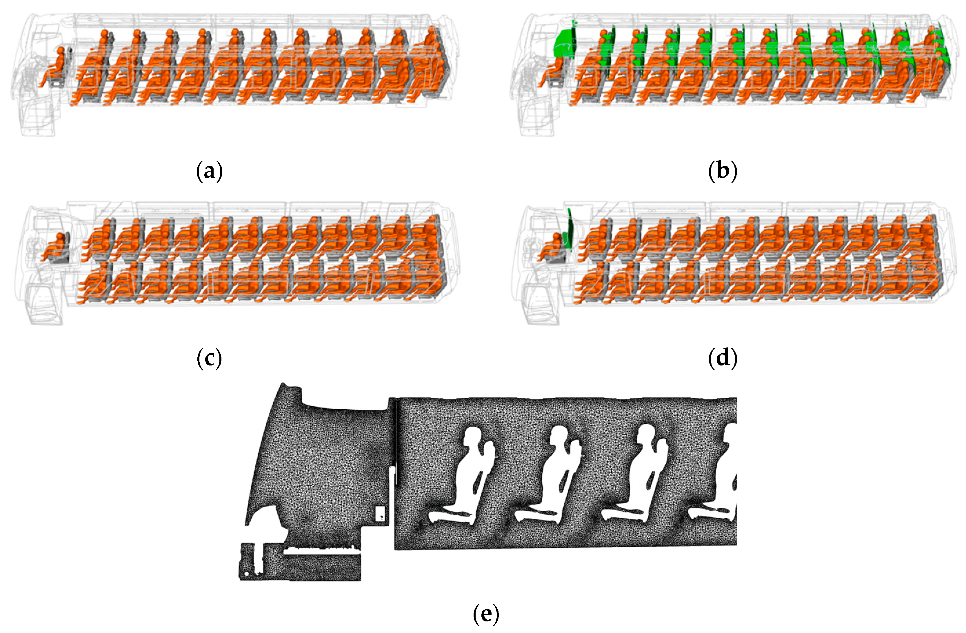
In this study, two types of bus cabin models were prepared as the targets of the numerical analyses. Figure 1 shows the outline of bus cabins (Models A and B) used in this study and the HVAC layout of each bus cabin. These two highway bus models are competing models of the same size sold by different Japanese automobile manufacturers, with slight differences in interior space volume and number of passengers. The geometries of bus cabins include the cabin space of the drivers and passengers, seats, windows, and HVAC inlets/outlets. Model A has 45 passenger seats and 1 driver seat in a bus cabin with a 40.0 m3 interior volume and Model B has 49 passenger seats and 1 driver seat, and an interior volume of 41.8 m3. The layout of the HVAC inlets is evenly spaced corresponding to the layout of the passenger seats. The main HVAC outlets are in the center and rear of the ceiling. In this study, considering the typical operation condition of Model A in real situations, 2308 m3/h of HVAC inflow rate was assumed, and an identical flow rate was set for Model B for comparative analysis under the same environmental condition.
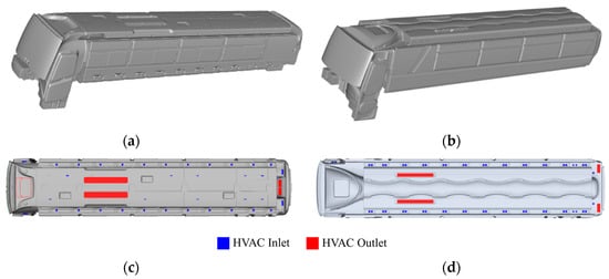
Figure 1.
Exterior geometry of the highway bus cabins and HVAC layouts: (a) Model A, (b) Model B, (c) HVAC layout of Model A, and (d) HVAC layout of Model B.
This study aimed to investigate the impact of the location of passengers in relation to one another on the infection risks in the entire bus cabin. The CSPs were located in all seats, as in the full-load condition shown in Figure 2. In addition, to examine effective methods for infection risk control, partition installations were considered as a passive countermeasure for infection risks. The infection risk analysis targeting both bus cabins had the following parametric cases: standard condition (without partitions), and the alternative condition (with partitions). In Model A, partitions were located between all passengers and the driver to confirm the impact of partitions on infection risks in the entire bus cabin. In Model B, only one partition was placed, behind the driver, focusing on the prevention of infection spread between passenger and driver cabins.
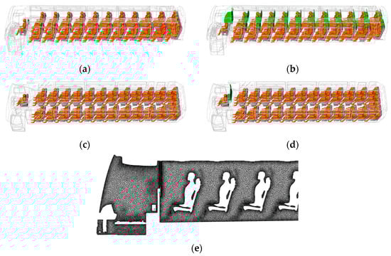
Figure 2.
Interior geometry of bus cabins including CSPs and partitions: (a) Model A, (b) Model A with partitions, (c) Model B, (d) Model B with a partitions, and (e) a representative grid design inside a bus cabin. CSPs and partitions are indicated in orange and green respectively.
2.2. CSP
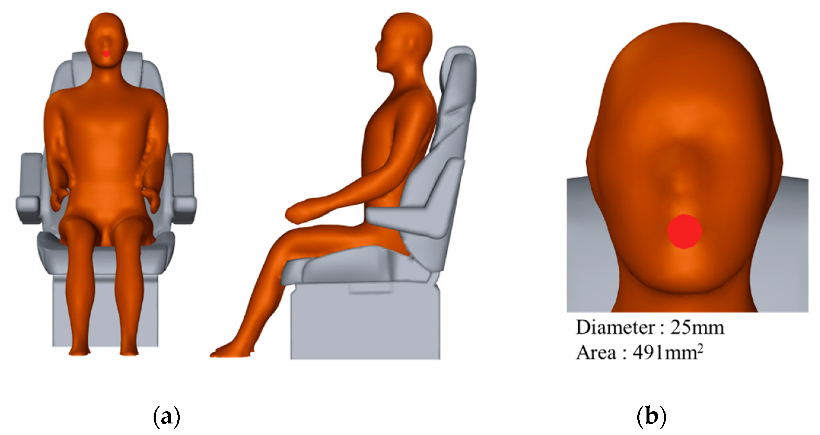
In this study, the CSPs—previously developed computational human models with a detailed body geometry in seated posture—were used to reproduce the microclimate around the passengers/drivers and the thermal environmental interaction between the bus cabin environment and the human body [24]. Figure 3 shows the outline of the CSP located in each passenger seat. To precisely reproduce the airflow pattern including thermal plume around the human body, the metabolic heat generation of the human body was applied based on the fundamental thermoregulation model, the 1-node model proposed by Fanger [25]. As shown in Figure 2e, high-density unstructured tetrahedral meshes were arranged around the CSP based on the triangular surface meshes on the CSP. The analytical grid around the contact region between CSPs and seats was smoothly trimmed to secure quality grids. The width, depth, and height of the CSP were approximately 0.5, 0.8, and 1.2 m, respectively, and the total area of the CSP surface that was in contact with air was 1.17 m2. Considering the great computational load due to the huge number of analytical grids in bus cabins, the detailed geometries of clothing were not reproduced, and mathematical modeling of clothing in the thermoregulatory analysis was considered instead.
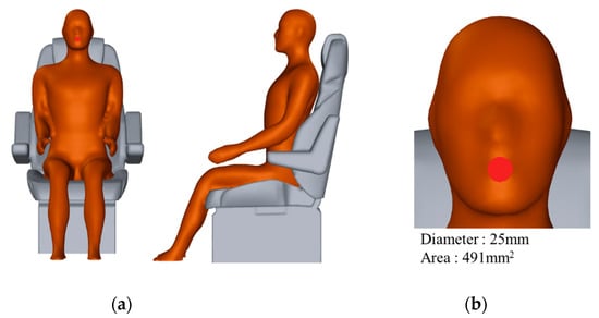
Figure 3.
(a) CSP outline in seated posture indicated in orange and (b) simplified mouth opening while coughing indicated in red.
2.3. Airflow, Heat, Moisture, and Droplet Transport Analysis
Equations (1) and (2) represent the Reynolds-averaged Navier–Stokes (RANS) equations for incompressible airflow analysis. The variables with an overline denote the ensemble-averaged variable. Ui [m/s] indicates the velocity of u, v, and w components, ρ [kg/m3] is the density of air, P [kg/m s2] is the pressure, ν [m2/s] and νt [m2/s] denote the kinematic viscosity and turbulent viscosity of air, respectively, gi [m/s2] is the gravity component of the acceleration vector in the i direction, β [-] represents the thermal expansion coefficient for buoyancy analysis, and ΔT is the temperature difference relative to the representative temperature. The density preservation law (mass conservation law) assuming a constant density is expressed by the continuity equation shown in Equation (1). The momentum law derived from Newton’s second law is represented by the Navier–Stokes equation with the buoyancy term represented in Equation (2). Additionally, the indoor turbulent flow is analyzed using the shear stress transfer (SST) k-ω turbulence model, which has an acceptable prediction accuracy for general indoor climate analysis [26].
The heat and moisture transfer can be expressed by Equations (3) and (4), respectively, using the flow field analysis. Here, T is the air temperature, α [m2/s] indicates the thermal diffusivity, S [K/s] and S’ [kg/kg’ s] represent the generation of heat and moisture, respectively, φ [kg/kg’] denotes the water vapor concentration in air, Dw [m2/s] is the diffusivity of water vapor in air, and σt [-] and σ [-] are the turbulent Prandtl number and turbulent Schmidt number, respectively.
Droplet transport is analyzed based on the Eulerian–Lagrangian method [27]. The particle force balance equation is expressed as Equation (5), where u’ [m/s] and Up [m/s] are the fluctuation components of velocity and particle velocity, respectively. The first term on the right-hand side represents the drag force of the particle, and the second term on the right-hand side represents the gravitational force; τ [s] is the particle relaxation time, dp [m] is the particle diameter, and ρp [kg/m3] is the particle density. CD [-] is the drag coefficient of the particle with the general correlation for spherical particles assuming droplets, and it is defined by Equation (7), when 0.01 < Rep ≤ 20 [28]. Rep [-] represents the relative Reynolds number, which is determined using Equation (8), and μ [kg/m s] is the dynamic viscosity of air.
To reproduce the particle dispersion in turbulent airflow, a discrete random walk model is applied. The fluctuating component of instantaneous velocity () is obtained using Equation (9). Here, represents a Gaussian random number. And from Equation (10), the local root mean square velocity fluctuation is obtained, assuming isotropic and locally uniform turbulent behavior of the particle.
The droplet diameter change and temperature decrease by vaporization are also considered in the particle transport analysis coupled with heat and moisture transfer analysis in a bus cabin. Here, r [m] denotes the radius of the droplet, Mw [kg/kg-mol] is the molecular weight of the droplet, Sc [-] is the Schmidt number for water vapor, φair and φp [kg/kg’] represent the water vapor concentration in the ambient air and on the droplet surface, respectively, mp [kg] is the mass of the droplet, cp [J/kg K] is the specific heat capacity of the particles, h [W/m2 K] is the convective heat transfer coefficient, Ap [m2] is the surface area of the particles, Tair and Tp [K] are the temperature in the ambient air and on the particle surface, respectively, and hfg [J/kg] is the latent heat of water. The water vapor concentration and temperature in the ambient air, φair and Tair in Equations (11) and (12), were determined based on the analysis results of temperature and humidity distribution in bus cabins calculated using Equations (1)–(4).
2.4. Analytical and Boundary Conditions
The analytical and boundary conditions used in the series of numerical analyses in this study are summarized in Table 1. Before the numerical analysis, a measurement experiment was performed in real bus cabins for Model A and B to obtain data on HVAC flow rates used for setting inflow boundary conditions. The flow rate distributions in the entire inlet openings were reproduced based on the measured data of each bus cabin. For comparative analyses under identical conditions between Model A and B, the total flow rate of the HVAC system in Model B was set proportional to that of Model A based on the flow rate in all inflow boundaries. We assumed highway bus services in summer; the cooling operation of the HVAC system and inflow temperature were set to 21.3 °C. The thermal loads in bus cabins by solar radiation were calculated using the solar ray tracing method with the sun direction vector at 12:00 p.m. on 21 June, in Tokyo. The bus cabins were assumed to be headed north. The long-wave radiation heat transfer was calculated using the surface-to-surface (S2S) model with view factor analysis [29].

Table 1.
Analytical and boundary conditions used in this study.
Four analytical cases (A1, A2, B1, and B2) were set corresponding to the type of bus cabin model and presence/absence of partitions. Identical loading rates of passengers and ventilation airflow rates were considered for all analytical cases; however, the total number of passengers and the spatial structures in the cabins were different owing to the difference in target bus cabins. In addition to the cases analyzed for examination of the impact of partitions on the infection risks, additional cases assuming mask-wearing based on Cases A1 and B1 were analyzed. The mask-wearing condition was introduced as an individual countermeasure, which plays a role in source control, and the function of personal protection by mask-wearing was not considered.
Table 2 summarizes the distribution of the number of droplets, initial droplet diameter (dpi), and droplet core diameter (dpc) adopted for numerical analysis [30]. The sizes of droplet nuclei were determined based on the ratio of the water component (98.2%) to non-volatile solid compounds (1.8%), assuming a saliva/phlegm droplet [31]. A total of 10,908 and 295 particles were generated assuming coughing without a mask and with a mask, respectively, considering limited computational resources. Particles were released from the simplified mouth opening of a coughing person, with a diameter of 25 mm, shown in Figure 3b. The initial particle velocity of 8.0 m/s was set for cases without masks, and the reduced initial velocity of 0.8 m/s was applied for cases with masks to reproduce the obstruction of coughing airflow and droplet dispersion by the mask [32]. The exhalation temperature was set to 309.4 K, which can be regarded as the core temperature of the human body. For the boundary condition of inhalation, a constant flow rate of 7.5 L/min was applied to the mouth openings. For the wall treatment of particles, trap boundary conditions were applied for all wall surfaces in bus cabins including CSP, and escape boundary conditions were set for all mouth openings and exhaust outlets in bus cabins.
Table 2.
Diameter distribution of droplets generated by coughing.
For precise prediction of the microclimate around CSPs, grid independence was carefully checked based on the suggested methodology in previous studies [9,33,34,35,36,37,38,39,40]. Six grid designs around CSPs were prepared with variations in grid resolution, and grid independence was carefully tested based on the analysis results of the coefficient of variation of the root mean square error (CV (RMSE)) and coefficient of determination (R2) [41]. This grid generation method was applied to the entire space in bus cabins, and the entire grid designs, with sufficiently high grid density, were prepared. The total number of final grid designs for each bus cabin model that have passed the additional grid independence tests targeting bus cabin spaces is approximately 50 million. We introduced a methodology of human microclimate analysis that was validated in the previous study based on the benchmark test with thermal manikin experiments [42]. In the series of numerical analyses, a semi-implicit method for pressure-linked equations (SIMPLE) was used, and a second-order upwind discretization scheme was used for convection analysis. These numerical methods have been widely used for indoor CFD analysis. Eulerian–Lagrangian particle transport analyses were conducted with sufficiently short timesteps (0.001 s). ANSYS Fluent (Ver. 2022R2) was used for numerical analyses in this study, and the solver settings and boundary conditions were carefully checked according to guidelines and benchmark tests for indoor CFD applications. Finally, we carefully conducted our CFPD (computational fluid and particle dynamics) analysis in accordance with the previously reported indoor CFD guidelines [9,37,38,39,40].
3. Results and Discussions
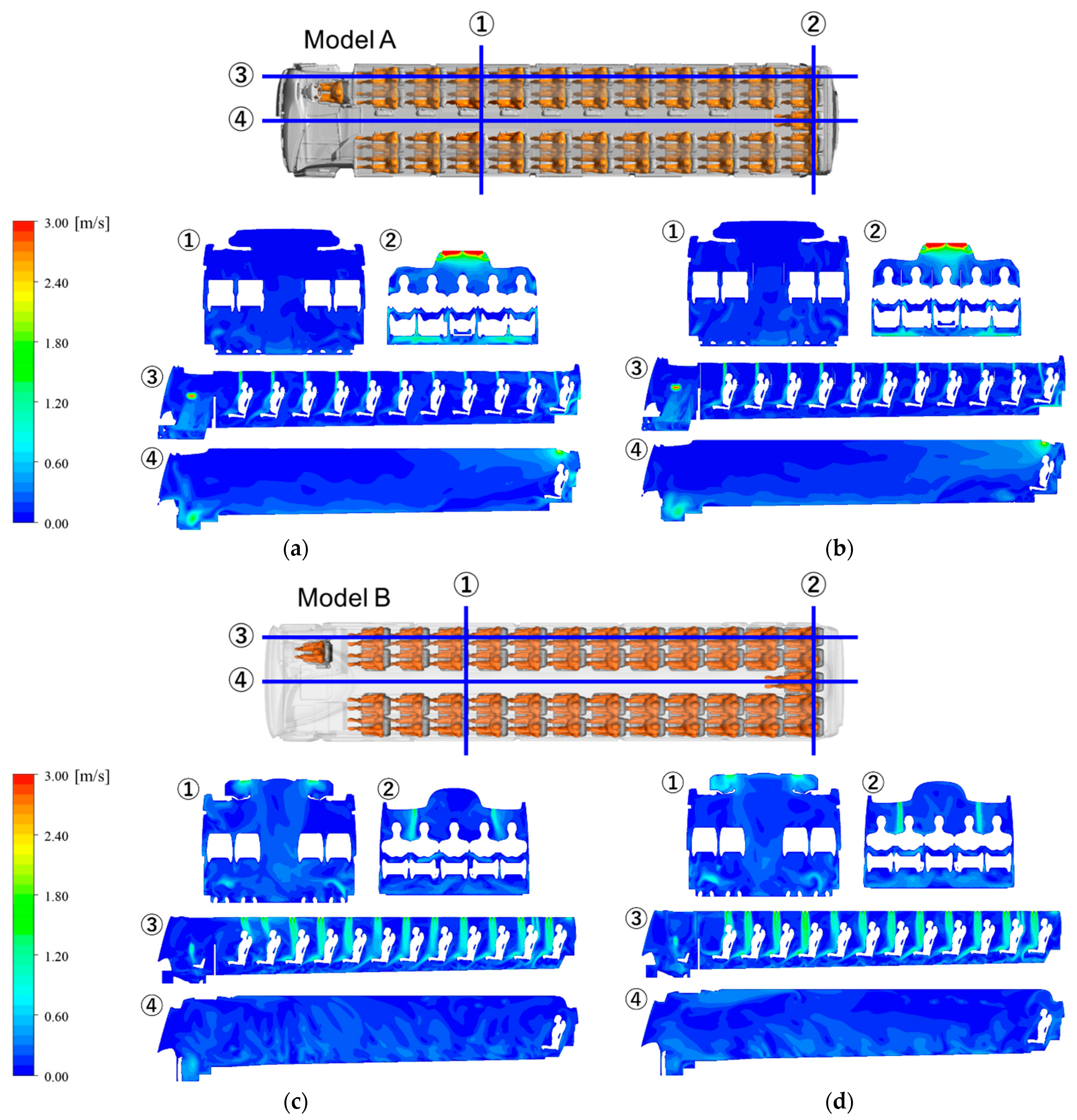
The analysis results of the steady-state scalar velocity distribution for Cases A1, A2, B1, and B2 are represented in Figure 4. The environmental analysis results for Cases A3 and B3 are identical to those of Cases A1 and B1 because the boundary conditions for environmental analysis in the bus cabins were identical. In all of the analytical cases, non-uniform airflow and temperature distributions were clearly identified inside the bus cabins, and jets of airflow were formed in the bus cabins according to the layout of the HVAC inlets. At the cross-section at window-side seats, the downward jets directed at each passenger were clearly observed, while a relatively stagnant airflow pattern was confirmed at the cross-section at the aisle in the center. Regarding the basic flow structure in both bus cabin models, downward HVAC inflows reached all of the passengers, flowed to the aisle area, and were finally exhausted through the HVAC outlets on the ceiling. On the ceiling were high-velocity local regions where the HVAC outlets are placed. Regarding the impact of partitions on the airflow patterns in bus cabins, no significant difference between Cases A1 and A2 was observed, since the main flow directions around partitions were on the vertical axis and upright partitions did not obstruct or block the airflow. In Model B, the partition behind the driver blocked the airflow from the driver cabin to the passenger cabin, and this affected the local flow pattern and HVAC inflow jet in the first and second rows of seats behind the driver cabin. Since the partition in Model B was located behind the driver only, no critical differences in the airflow pattern of the entire bus cabin between Cases B1 and B2 were observed.
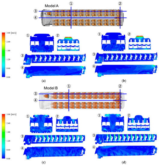
Figure 4.
Flow field analysis results inside bus cabins. (a) Case A1, (b) Case A2, (c) Case B1, and (d) Case B2. The circled numbers indicate the location of cross-sections highlighted in blue lines.
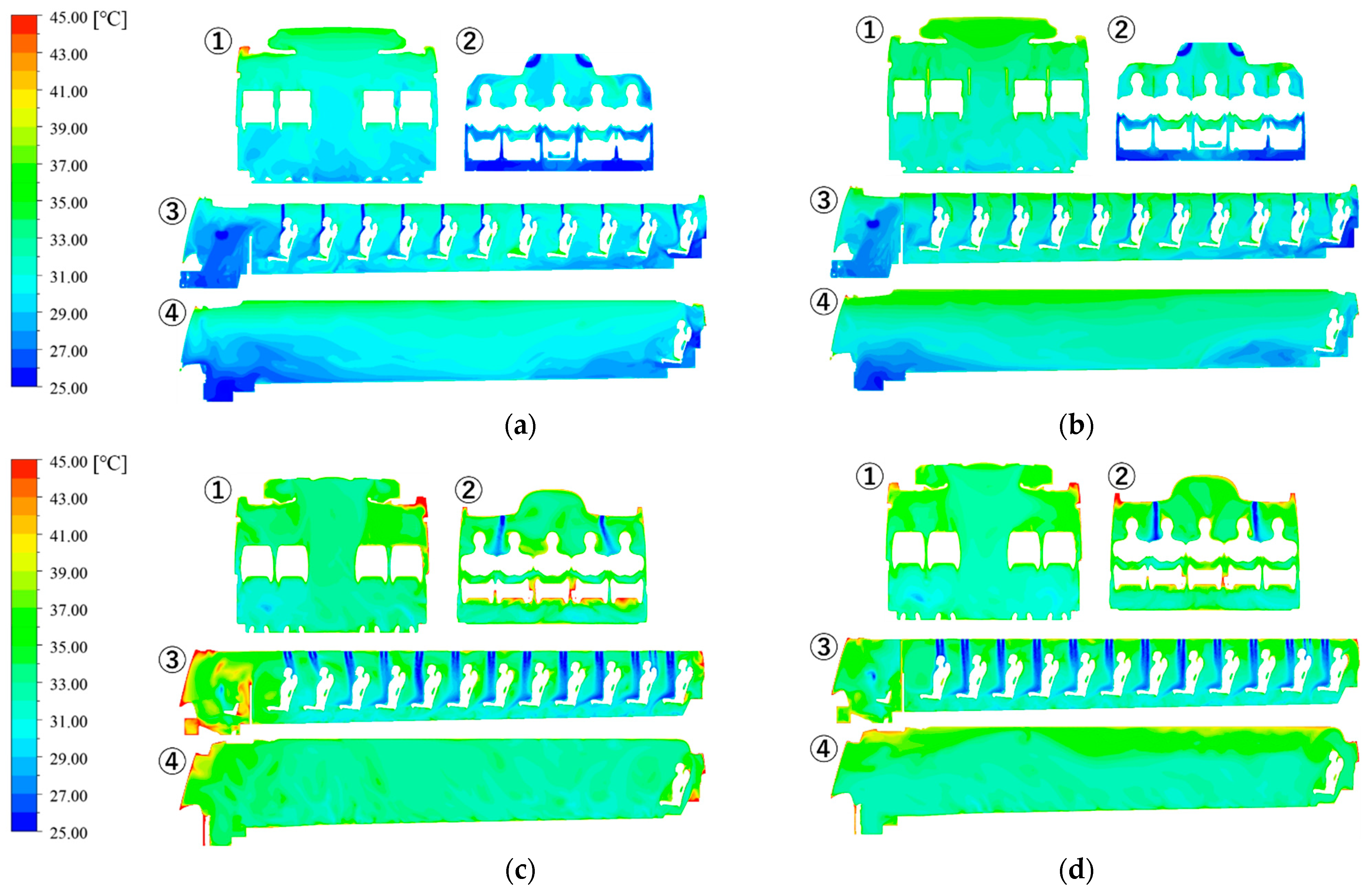
The results of the heat transfer analysis for bus cabins are shown in Figure 5. Regarding the overall characteristic of temperature distribution, the individual local climate was observed according to the regular geometry and HVAC layout of both of the bus cabin models. A high-temperature distribution and thermal plume were formed around the CSPs based on human heat generation. For Model A, a different tendency of temperature distribution between Case A1 and A2 was observed. In Case A2, a clearer local climate was formed due to the partitions between individual spaces. This led to the development of thermally stagnant regions around CSPs, due to the blocked convective and radiative heat transfer by the partitions. Model B had a higher temperature distribution in the driver cabin in Case B2 compared to that of Case B1 due to the partition behind the driver trapping heat in the driver cabin. In addition, a higher overall temperature was observed in Model B, which had more passengers and total human heat generation under identical ventilation flow rates.
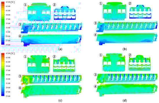
Figure 5.
Temperature distribution inside bus cabins. (a) Case A1, (b) Case A2, (c) Case B1, and (d) Case B2. The circled numbers indicate the location of cross-sections highlighted in blue lines in Figure 4.
In addition to the representative environmental factors in bus cabins, the analysis of ventilation effectiveness was conducted based on Scale for Ventilation Efficiency 3 (SVE3) [43]. SVE3 is widely used in the field of indoor environmental design since it can predict the spatial distribution of ventilation effectiveness in indoor spaces. Its value denotes the traveling time of airflow from the supply inlets to the target calculation point; therefore, it is also called “age of air.” As a calculation method, passive scalar (as a tracer gas) is uniformly generated in the entire bus cabin, and assuming fresh air inflow from the supply inlets, the concentration distribution of the passive scalar is analyzed using Equation (17).
where C [-] denotes the concentration of the passive scalar, DC [m2/s] is the diffusion coefficient of the passive scalar, and S″ represents the source term of the passive scalar. It is defined for the uniform generation of passive scalar in the bus cabin.
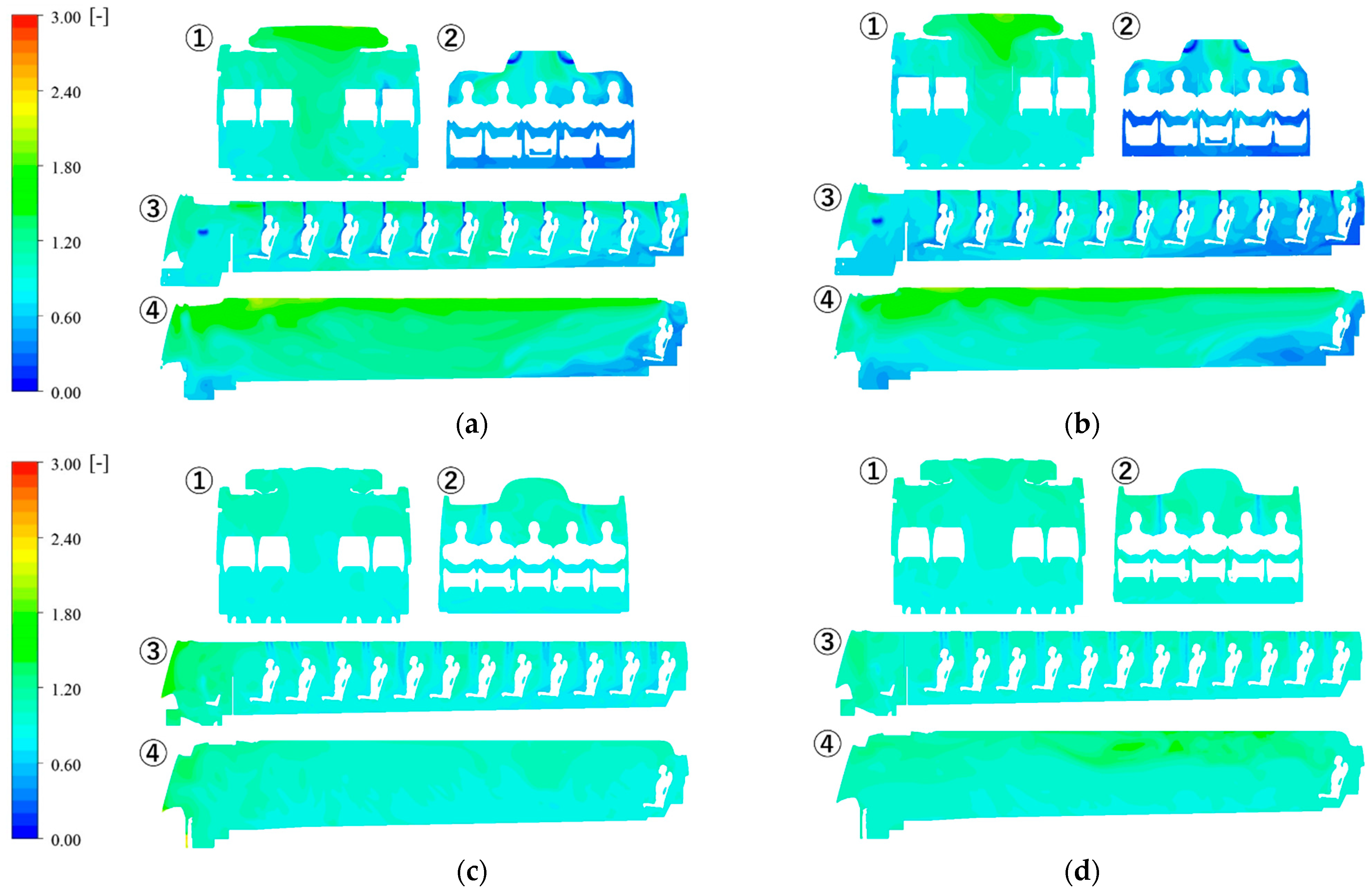
Figure 6 shows the spatial distribution of SVE3 in bus cabins. The nominal time constants of Models A and B are 62.4 s and 65.2 s, respectively, and these values correspond to SVE3 values of 1.0 in each model. A region with a high SVE3 value is a stagnant airflow region, and vice versa. The volume-averaged SVE3 was 1.01 in Case A1, 0.92 in Case A2, 0.97 in Case B1, and 1.0 in Case B2. Model B had an almost uniform distribution of SVE3, while non-uniformity, including a higher SVE3 region in the ceiling and lower SVE3 region in the rear side, was observed in Model A. This was caused by the differences in HVAC layout and spatial structure in the bus cabins. In addition, it was revealed that the impact of partitions on the SVE3 distribution in the entire bus cabin was insignificant, while the partitions slightly reduced the SVE3 around passengers.
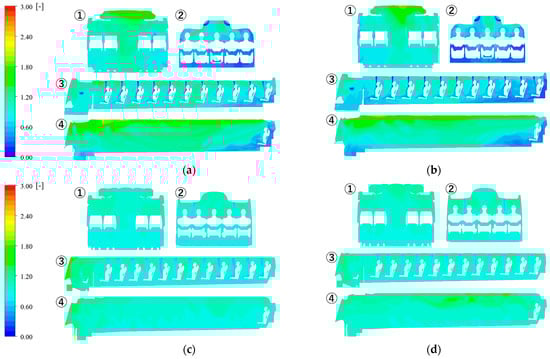
Figure 6.
SVE3 distribution inside bus cabins. (a) Case A1, (b) Case A2, (c) Case B1, and (d) Case B2. The circled numbers indicate the location of cross-sections highlighted in blue lines in Figure 4.
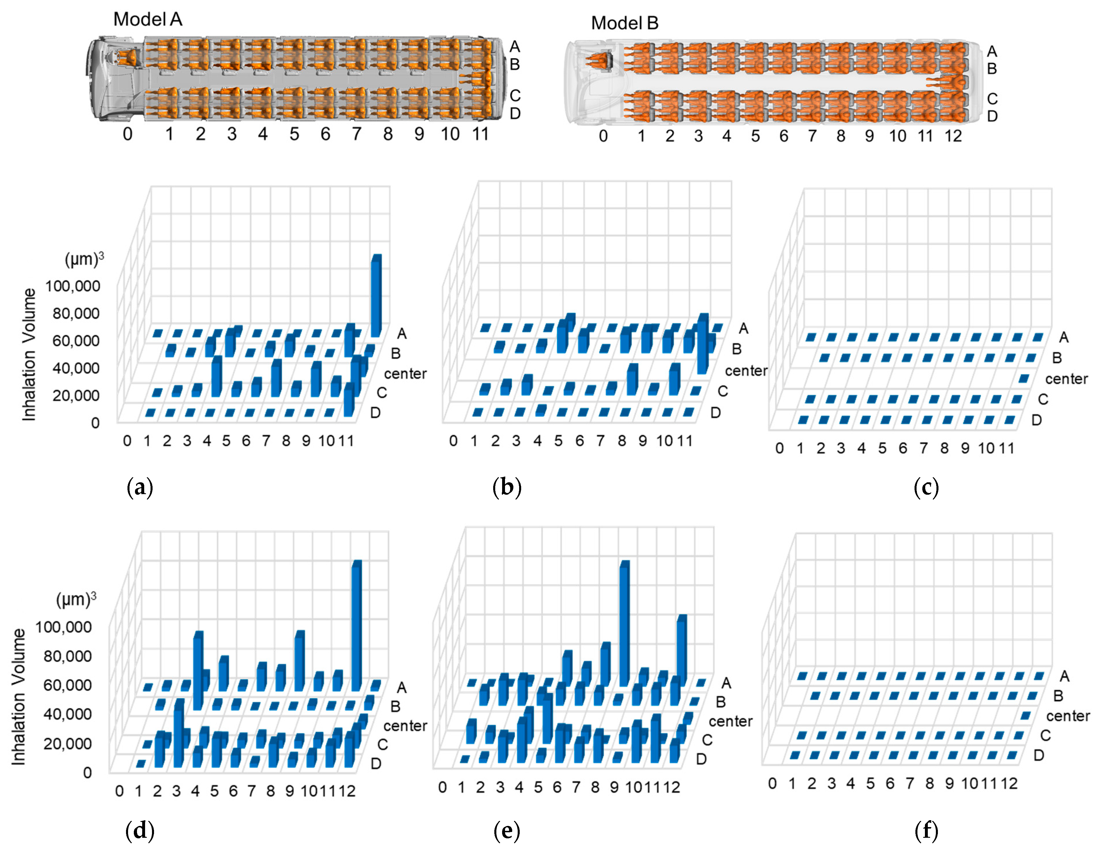
Based on the results of the analysis of the flow field in bus cabins, an Eulerian–Lagrangian particle transport analysis was conducted, and the average volume of the droplet inhaled by each passenger was analyzed (summarized in Figure 7). A series of particle transport analyses, assuming the droplet diffusion of a cough generated by each passenger and driver, were conducted for the overall estimation of the infection risk targeting all of the passengers and the driver. The results were averaged over the entirety of the analytical cases (46 for Model A, and 50 for Model B) to estimate the overall distribution of individual infection risks. The height of each bar (Figure 7) indicates the average volume of inhaled droplets by each passenger. The passengers who inhaled the largest volume of droplets in Model A were concentrated in the aisle-side seats, while those in Model B were concentrated in the window-side seats. These differences were caused by differences in the flow structure in each bus cabin. In addition, the results show that, relatively, many more droplets were inhaled in Model B.
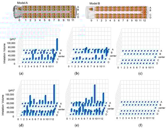
Figure 7.
Average volume of inhaled droplet: (a) Case A1, (b) Case A2, (c) Case A3, (d) Case B1, (e) Case B2, and (f) Case B3. The numbers of 0-12 and letters of A-D indicate the location of rows and columns of seats in bus cabins.
Regarding the impact of partitions, a remarkable decrease in inhaled volume in the entire bus cabin was experienced in Model A, while there was no significant impact of partitions in Model B due to the number and location of passengers. In addition, differences in the overall distribution of the inhaled volume between cases with and without partitions were observed in both models, due to the changes in the flow field.
Finally, droplet dispersion analyses were conducted under the mask-wearing condition, which was introduced as an individual countermeasure for infection risk in bus cabins; the results are summarized in Figure 7c,f. Almost none of the droplets were inhaled by each passenger due to the dramatically reduced droplets generated by coughing. An extremely small volume of droplets reached the breathing area of some passengers/the driver. These results show that wearing masks is an effective countermeasure to control infection risk, regardless of the type of bus cabin model.
Based on the analysis results of the droplet inhalation volume, the infection risk distribution in the bus cabin was estimated using Equations (14)–(16), where Dq1 is the dose of quanta for infection [quanta], cv is the viral load in the droplet [RNA copies/mL] and ci is the conversion coefficient from the number of RNA copies to quanta [quanta/RNA copies], Respectively, and VI is the average volume of droplets generated by another passenger/driver and inhaled by the target person [mL] (summarized in Figure 8). SARS-CoV-2 airborne infection was assumed, and 109 for cv and 0.02 for ci were applied based on previous studies on SARS-CoV-2 infection [44,45,46,47]. Equation (15) is widely known as the Wells-Riley equation, which is an exponential dose-response model that estimates the probability of infection, PI [-]. is the average infection risk of the target passenger [-], calculated by , the infection probability of target passenger averaged by the total number of passengers including the driver, except the target person [-], and , the probability of occurrence of each Dq1 value [-]. We applied as 1.0 to consider the infection occurrence with a single cough by each passenger.
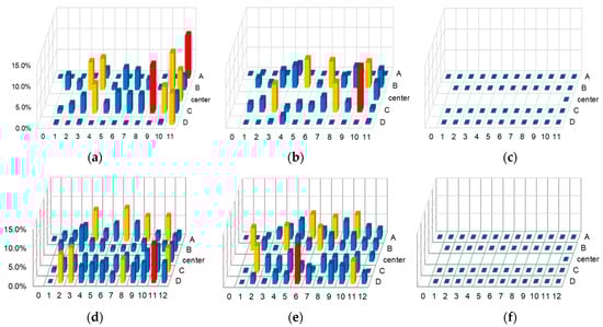
Figure 8.
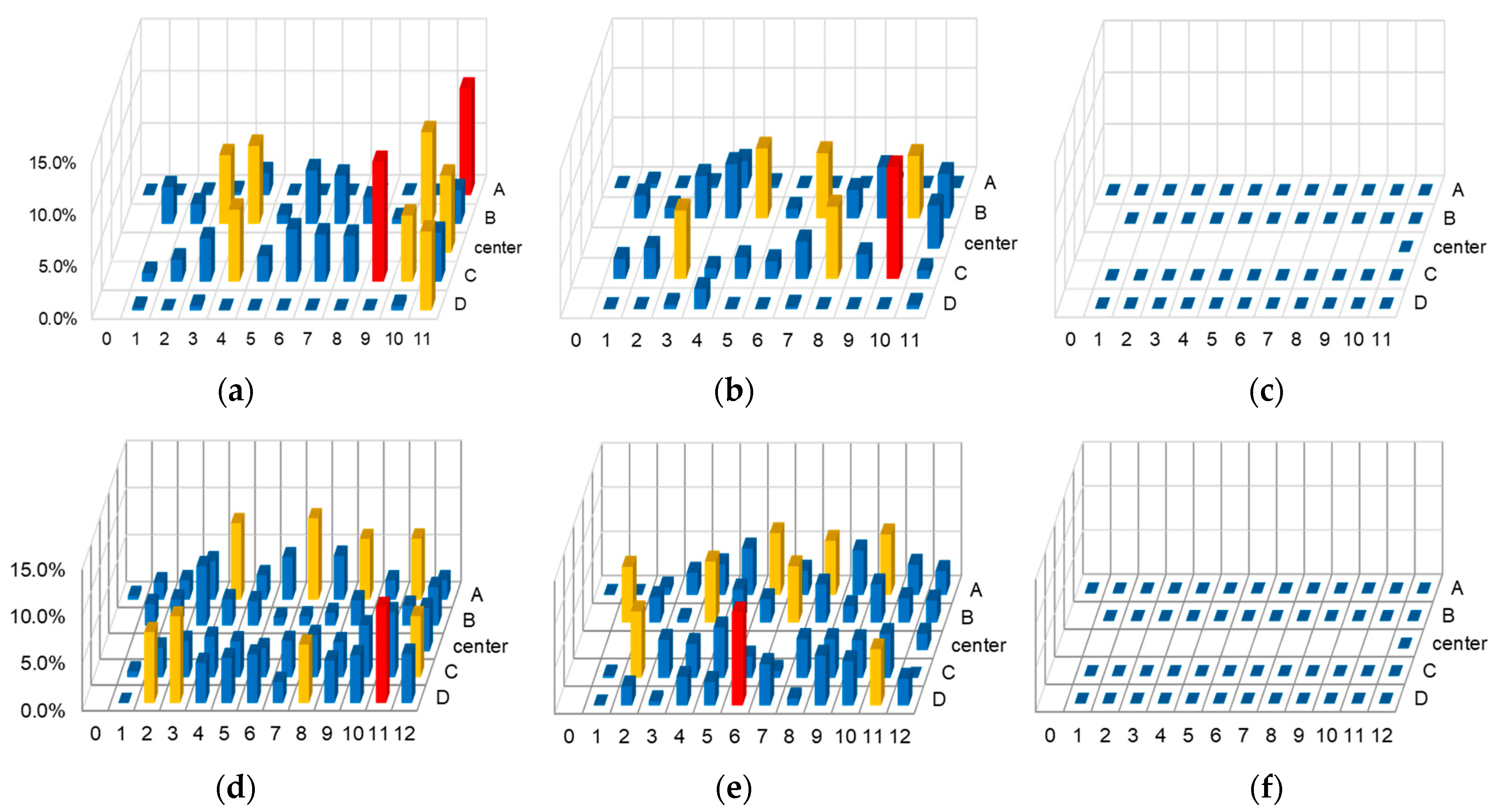
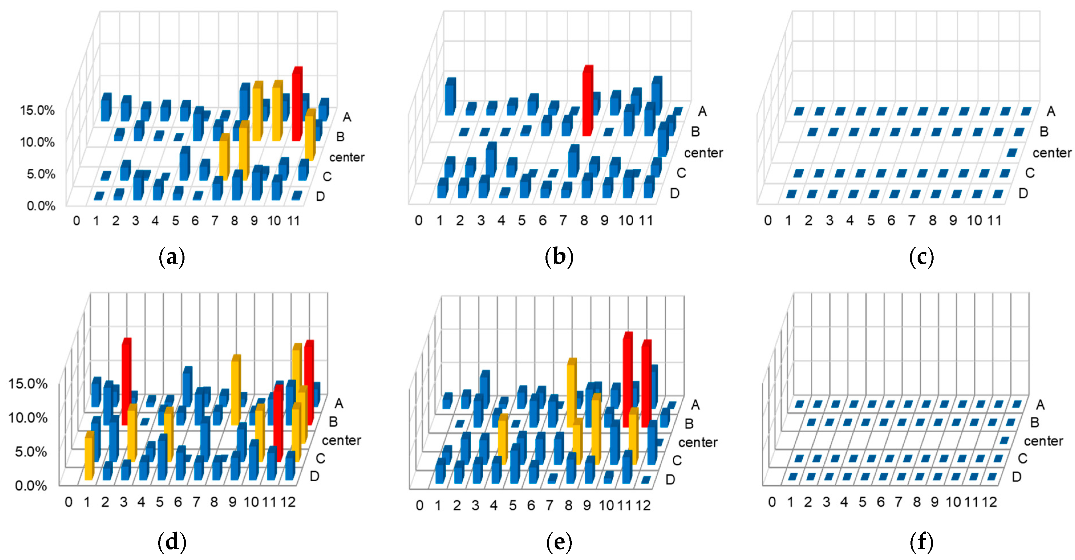
Infection risk distribution in bus cabins: (a) Case A1, (b) Case A2, (c) Case A3, (d) Case B1, (e) Case B2, and (f) Case B3. The numbers of 0-12 and letters of A-D indicate the location of rows and columns of seats in bus cabins highlighted in Figure 7. The blue, yellow, and red bars indicate infection risks of less than 5%, 5~10%, and over 10%, respectively.
Figure 8 shows spatial distributions of the averaged infection risk in the bus cabins. The average infection risk for all of the passengers and the driver was 2.8% without partitions and 2.2% with partitions in Model A; and 4.1% without partitions and 3.6% with partitions in Model B. The distribution tendency of the inhaled droplet volume and infection risk were generally consistent. However, they did not always coincide due to Equation (2), which is non-linear and dominantly affected by the inhalation volume of droplets, which varied in all coughing scenarios for each passenger and the driver. In Model A, the overall decrease in infection risk as an effect of partitions was clearly observed. In addition, the result of the mask-wearing scenario showed a 0% average infection risk, and the complete prevention of airborne infection by mask-wearing was confirmed. Thus, wearing masks is a sure countermeasure to control the airborne infection risk, and partitions are also effective as a passive countermeasure. Similar to the result of the volume distribution of inhaled droplets, passengers on aisle-side seats showed higher infection risk distribution in Model A. An improvement by partitions was not found in Model B, while a decrease in infection risks for passengers around the partitions was observed. A higher infection risk distribution was found in aisle-side seats in Model A and window-side seats in Model B, as shown in the analysis results of the inhaled droplet volumes, and it was revealed more clearly that the flow structure of the HVAC design has a certain impact on the spatial distribution of the infection risk in the bus cabin. Regardless of the spatial structure or flow field characteristics in the bus cabin, mask-wearing was confirmed to reduce the infection risk.
On the other hand, the infection spread risk was also investigated, based on Equations (17)–(19), by a reversed approach of the infection risk assessment method. Here, Dq2 is the dose of quanta for infection spread [quanta], and VS is the volume of droplets inhaled by other passengers and the driver from the droplets generated by the target person [mL]. PS indicates the probability of infection spread, [-]. is an average infection spread risk of the target passenger [-], calculated by , the infection spread probability of the target passenger averaged by the total number of passengers/driver except the target person.
Figure 9 summarizes the spatial distributions of the averaged infection spread risk in the bus cabins. In contrast to the results of the infection risk assessment, the passengers with a high infection spread risk were not concentrated in the aisle-side seats in Model A and window-side seats in Model B. In other words, there is no direct correlation between the spatial distribution of the infection risk and the infection spread risk. In Model A, a significant improvement in infection spread risk with partitions was confirmed, while a decrease in infection spread risks was observed for the driver and passengers around the partitions only. The overall average infection spread risks in each case are identical to the infection risk since the totals of VI and VS in each analytical case are identical.
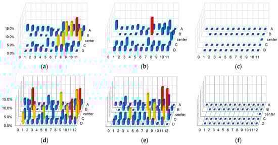
Figure 9.
Infection spread risk distribution in bus cabins: (a) Case A1, (b) Case A2, (c) Case A3, (d) Case B1, (e) Case B2, and (f) Case B3. The numbers of 0-12 and letters of A-D indicate the location of rows and columns of seats in bus cabins highlighted in Figure 7. The blue, yellow, and red bars indicate infection spread risks of less than 5%, 5~10%, and over 10%, respectively.
By comparing the level of infection spread risk in Models A and B, it can be seen that Model B showed an overall higher infection spread risk. The risks around partitions, including the driver, were reduced due to the partition in Model B, while there was no significant improvement in the rest of the entire space. Regarding both infection and infection spread, it was revealed that complete risk reduction can be achieved by mask-wearing.
This study established a numerical prediction method for airborne infection risk in bus cabins and attempted to precisely predict the airflow pattern inside bus cabins based on CFD with a logical methodology and sophisticated geometry data including CSPs and bus cabin models, because the main factor influencing infection risks is the airflow characteristics in bus cabins. The overall results of our spatial distribution analysis of infection risk are related to the HVAC layout, especially the location of supply inlets and outlets in the ceiling, which determine airflow patterns in bus cabins and greatly influences the paths of droplet transport. For example, inflow jets in Model A were mainly directed toward the passengers in aisle-side seats, while those in Model B were mainly directed toward the passengers in window-side seats, and these are the areas of high infection risks in each bus cabin.
There are several limitations to this study. The climate in bus cabins is dominantly affected by the layout and operation of the HVAC system. However, this study assumed a single layout and operation condition of the HVAC systems. The HVAC systems of highway buses require the efficient layout of related mechanical equipment in a very limited space, e.g., underneath the ceiling or sub-floor space, and a good balance between supply inlets and exhaust outlets. In addition, the interior spaces of buses are mainly surrounded by glass surfaces and have very severe heat load conditions, making the constraints on the indoor environmental design very severe. Although this study has not been able to optimize the HVAC system in terms of indoor environmental quality, an alternative method is to install simple partitions at each seat, and it was quantitatively shown that the infection risk can be well controlled without significantly changing the HVAC efficiency. In the future, parametric studies could reveal the correlation between airborne infection risks and HVAC operation conditions, and could contribute to the further optimization of HVAC design for reducing infection risk in highway bus cabins. Furthermore, parametric analyses of airborne infection risk were performed as a demonstrative application of the infection risk assessment method in bus cabins, and further investigation through additional parametric studies could result in effective countermeasures for highway bus cabins in addition to the passive/individual countermeasures focused on in this study.
There is also the potential for improvement in the prediction accuracy of the human microclimate. This study adopted a basic thermoregulation model, the 1-node model proposed by Fanger. The total heat generation rate calculated by the 1-node model was applied uniformly across the whole skin surface of the CSP as a thermal boundary condition. The mathematical modeling of human thermoregulation has a long history, and several thermoregulation models, considering multi-node and multi-segment, have been developed [48,49,50,51]. These models also allow for advanced modeling of evaporative heat loss from the human body, which is simplified in this study. In addition, the modeling of clothing geometry was omitted considering its huge computational load. The complex geometry of clothing may have an impact on the flow characteristics around the human body and also in the breathing zone. Through upgrading the human thermoregulatory analysis and the modeling of clothing, the prediction accuracy of the human microclimate, including the breathing zone, could be improved.
The direct validation of the infection risk analysis in the bus cabin was not conducted in this study since the examination of the infection risks based on subject experimentation is prohibited for ethical reasons. However, for the prediction of the human microclimate and bus cabin environments, which has a decisive effect on the droplet transport path and infection risk distribution, reliable methodologies were adopted in each part of the comprehensive numerical analyses in this study. The methodology of human microclimate analysis using CSP was already validated in our previous study, and suggested methodologies for quality control of indoor CFD analysis were applied in the analyses of the bus cabin climate [30,52]. The benchmark test of environmental analysis in bus cabins could be performed based on the measured data of environmental factors in bus cabins.
4. Conclusions
This study developed a comprehensive prediction method for the bus cabin environment and airborne infection and spread risks. The digital twins of two types of bus cabins, including passengers, were prepared, and airflow, heat, moisture, and particle transport analyses for bus cabins were conducted based on CFD. Finally, the spatial distribution of the airborne infection risk and spread risk assuming SARS-CoV-2 infection were analyzed, and the effectiveness of representative passive/individual countermeasures for airborne infection was discussed. It was found that the spatial distribution of airborne infection/spread risks is affected by the HVAC layouts in different bus cabins. Partition installation as a passive countermeasure had a certain impact on the human microclimate, and decreased infection risks were observed. Finally, the almost complete prevention of airborne infection was confirmed with an individual countermeasure, mask-wearing. The comprehensive prediction method of airborne infection/spread risks established in this study could contribute to the optimal environmental design of bus cabins to control the infection/spread risks of airborne diseases.
Author Contributions
Conceptualization, S.-J.Y. and K.I.; methodology, S.-J.Y.; software, S.Y.; validation, S.-J.Y. and S.Y.; formal analysis, S.Y.; investigation, S.-J.Y.; resources, S.-J.Y.; data curation, H.P.; writing—original draft preparation, S.-J.Y.; writing—review and editing, S.-J.Y. and K.I.; visualization, H.P.; supervision, K.I.; project administration, K.I.; funding acquisition, S.-J.Y. and K.I. All authors have read and agreed to the published version of the manuscript.
Funding
This research was partially funded by the Japan Society for the Promotion of Science (JSPS) Grants-in-Aid for Scientific Research (KAKENHI) (grant numbers JP 22K18300, JP 22H00237, JP22K14371, JP 20KK0099, and JP21K14306), the Japan Science and Technology (JST), CREST Japan (grant number JP 20356547), FOREST program from JST, Japan (Grant number JPMJFR225R), and MEXT as “Program for Promoting Researches on the Supercomputer Fugaku” (JPMXP1020210316).
Data Availability Statement
No public or private data were used or analyzed in this study. The data used were generated by commercial software, thus data sharing is not applicable.
Conflicts of Interest
The authors declare no conflict of interest.
References
- Bagshaw, M.; Illig, P. The Aircraft Cabin Environment. In Travel Medicine; Elsevier: Amsterdam, The Netherlands, 2019; pp. 429–436. [Google Scholar]
- Shek, K.W.; Wai, T.C. Combined comfort model of thermal comfort and air quality on buses in Hong Kong. Sci. Total Environ. 2008, 389, 277–282. [Google Scholar] [CrossRef]
- Praml, G.; Schierl, R. Dust exposure in Munich public transportation: A comprehensive 4-year survey in buses and trams. Int. Arch. Occup. Environ. Health 2000, 73, 209–214. [Google Scholar] [CrossRef]
- Chan, A.T. Commuter exposure and indoor–outdoor relationships of carbon oxides in buses in Hong Kong. Atmos. Environ. 2003, 37, 3809–3815. [Google Scholar] [CrossRef]
- Chan, L.Y.; Lau, W.L.; Zou, S.C.; Cao, Z.X.; Lai, S.C. Exposure level of carbon monoxide and respirable suspended particulate in public transportation modes while commuting in urban area of Guangzhou, China. Atmos. Environ. 2002, 36, 5831–5840. [Google Scholar] [CrossRef]
- Guevara-Luna, M.; Belalcazar, L.; Guevara Luna, F. CFD Modeling and Validation of Tracer Gas Dispersion to Evaluate Self-Pollution in School Buses. Asian J. Atmos. Environ. 2019, 13, 1–10. [Google Scholar] [CrossRef]
- Zhu, S.; Demokritou, P.; Spengler, J. Experimental and numerical investigation of micro-environmental conditions in public transportation buses. Build. Environ. 2010, 45, 2077–2088. [Google Scholar] [CrossRef]
- Wang, C.; Yoo, S.-J.; Ito, K. Does detailed hygrothermal transport analysis in the respiratory tract affect skin surface temperature distributions using a thermoregulation model? Adv. Build. Energy Res. 2020, 14, 450–470. [Google Scholar] [CrossRef]
- Sorensen, D.N.; Nielsen, P.V. Quality control of computational fluid dynamics in indoor environments. Indoor Air 2003, 13, 2–17. [Google Scholar] [CrossRef]
- Xing, H.; Hatton, A.; Awbi, H.B. A study of the air quality in the breathing zone in a room with displacement ventilation. Build. Environ. 2001, 36, 809–820. [Google Scholar] [CrossRef]
- Brohus, H. Personal Exposure to Contaminant Sources in Ventilated Rooms. Ph.D. Thesis, Aalborg University, Aalborg, Denmark, 1997. [Google Scholar]
- Brohus, H.; Balling, K.D.; Jeppesen, D. Influence of movements on contaminant transport in an operating room. Indoor Air 2006, 16, 356–372. [Google Scholar] [CrossRef]
- Murakami, S.; Zeng, J. Flow and temperature fields around human body with various room air distributions, Part 1—CFD study on computational thermal manikin. AHSRAE Trans. 1997, 103, 3–15. [Google Scholar]
- Murakami, S.; Kato, S.; Zeng, J. Combined simulation of airflow, radiation and moisture transport for heat release from human body. Build. Environ. 2000, 35, 489–500. [Google Scholar] [CrossRef]
- Topp, C.; Nielsen, P.V.; Sørensen, D.N. Application of Computer-Simulated Persons in Indoor Environmental Modeling. ASHRAE Trans. 2002, 108 Pt 2, 2002. [Google Scholar]
- Gao, N.P.; Zhang, H.; Niu, J.L. Investigating indoor air quality and thermal comfort using a numerical thermal manikin. Indoor Built Environ. 2007, 16, 7–17. [Google Scholar] [CrossRef]
- Kuga, K.; Wargocki, P.; Ito, K. Breathing zone and exhaled air re-inhalation rate under transient conditions assessed with a computer-simulated person. Indoor Air 2022, 32, e13003. [Google Scholar] [CrossRef]
- Kuga, K.; Ito, K.; Chen, W.; Wang, P.; Kumagai, K. A numerical investigation of the potential effects of e-cigarette smoking on local tissue dosimetry and the deterioration of indoor air quality. Indoor Air 2020, 30, 1018–1038. [Google Scholar] [CrossRef]
- Murota, K.; Kang, Y.; Hyodo, S.; Yoo, S.-J.; Takenouchi, K.; Tanabe, S.; Ito, K. Hygro-thermo-chemical transfer analysis of clothing microclimate using three-dimensional digital clothing model and computer-simulated person. Indoor Built Environ. 2022, 31, 1493–1510. [Google Scholar] [CrossRef]
- Ito, K. In silico human model for fluid-initiated indoor environmental design. Indoor Built Environ. 2017, 26, 295–297. [Google Scholar] [CrossRef]
- Yoo, S.-J.; Ito, K. Assessment of Transient Inhalation Exposure using in silico Human Model integrated with PBPK–CFD Hybrid Analysis. Sustain. Cities Soc. 2018, 40, 317–325. [Google Scholar] [CrossRef]
- Yoo, S.-J.; Ito, K. Numerical Prediction of Tissue Dosimetry in Respiratory Tract using Computer Simulated Person integrated with physiologically based pharmacokinetic (PBPK)-computational fluid dynamics (CFD) Hybrid Analysis. Indoor Built Environ. 2018, 27, 877–889. [Google Scholar] [CrossRef]
- Yoo, S.-J.; Ito, K. Multi-stage optimization of local environmental quality by comprehensive computer simulated person as a sensor for HVAC control. Adv. Build. Energy Res. 2019, 14, 171–188. [Google Scholar] [CrossRef]
- Ito, K. Toward the development of an in silico human model for indoor environmental design. Proc. Jpn. Acad. Ser. B 2016, 92, 185–203. [Google Scholar] [CrossRef]
- Fanger, P.O. Thermal Comfort; McGraw-Hill Inc.: New York, NY, USA, 1973. [Google Scholar]
- Menter, F.R.; Kuntz, M.; Langtry, R. Ten years of Industrial experience with the SST turbulence model. In Turbulence, Heat and Mass Transfer; Hanjalic, K., Nagano, Y., Tummers, M., Eds.; Begell House, Inc.: Danbury, CT, USA, 2003; p. 625e632. [Google Scholar]
- Yan, Y.; Li, X.; Ito, K. Numerical investigation of indoor particulate contaminant transport using the Eulerian-Eulerian and Eulerian–Lagrangian two-phase flow models. Exp. Comput. Multiph. Flow 2019, 2, 31–40. [Google Scholar] [CrossRef]
- Clift, R.; Grace, J.; Weber, M.E. Bubbles, Drops, and Particles; Dover Publications, Inc.: Mineola, NY, USA, 2005. [Google Scholar]
- ANSYS/Fluent. 15 User’s Guide; ANSYS, Inc.: Canonsburg, PA, USA, 2013. [Google Scholar]
- Xie, X.; Li, Y.; Sun, H.; Liu, L. Exhaled droplets due to talking and coughing. J. R. Soc. Interface 2009, 6 (Suppl. S6), 703–714. [Google Scholar] [CrossRef]
- Nicas, M.; Nazaroff, W.W.; Hubbard, A. Toward Understanding the Risk of Secondary Airborne Infection: Emission of Respirable Pathogens. J. Occup. Environ. Hyg. 2005, 2, 143–154. [Google Scholar] [CrossRef]
- Simha, P.P.; Rao, P.S.M. Universal trends in human cough airflows at large distances. Phys. Fluids 2020, 32, 081905. [Google Scholar] [CrossRef] [PubMed]
- Yoo, S.; Ito, K. Validation, verification, and quality control of computational fluid dynamics analysis for indoor environments using a computer-simulated person with respiratory tract. Jpn. Archit. Rev. 2022, 5, 714–727. [Google Scholar] [CrossRef]
- Foat, T.G.; Parker, S.T.; Castro, I.P.; Xie, Z.-T. Numerical investigation into the structure of scalar plumes in a simple room. J. Wind Eng. Ind. Aerodyn. 2018, 175, 252–263. [Google Scholar] [CrossRef]
- Nielsen, P.V. Specification of a two-dimensional test case. In IEA; Institut for Bygningsteknik, Aalborg Universitet: Aalborg, Denmark, 1990; Volume 1, p. R9040. [Google Scholar]
- Nielsen, P.V. Fifty years of CFD for room air distribution. Build. Environ. 2015, 91, 78–90. [Google Scholar] [CrossRef]
- Ito, K.; Inthavong, K.; Kurabuchi, T.; Ueda, T.; Endo, T.; Omori, T.; Ono, H.; Kato, S.; Sakai, K.; Suwa, Y.; et al. CFD benchmark tests for indoor environmental problems: Part 1 isothermal/non-isothermal flow in 2D and 3D room model. J. Archit. Eng. Technol. 2015, 2, 1–22. [Google Scholar]
- Ito, K.; Inthavong, K.; Kurabuchi, T.; Ueda, T.; Endo, T.; Omori, T.; Ono, H.; Kato, S.; Sakai, K.; Suwa, Y.; et al. CFD benchmark tests for indoor environmental problems: Part 4 air-conditioning airflows, residential kitchen airflows and fire-induced flow. J. Archit. Eng. Technol. 2015, 2, 76–102. [Google Scholar]
- Ito, K.; Inthavong, K.; Kurabuchi, T.; Ueda, T.; Endo, T.; Omori, T.; Ono, H.; Kato, S.; Sakai, K.; Suwa, Y.; et al. CFD benchmark tests for indoor environmental problems: Part 3 numerical thermal manikins. J. Archit. Eng. Technol. 2015, 2, 50–75. [Google Scholar]
- Ito, K.; Inthavong, K.; Kurabuchi, T.; Ueda, T.; Endo, T.; Omori, T.; Ono, H.; Kato, S.; Sakai, K.; Suwa, Y.; et al. CFD benchmark tests for indoor environmental problems: Part 2 cross-ventilation airflows and floor heating systems. J. Archit. Eng. Technol. 2015, 2, 23–49. [Google Scholar]
- Lee, M.; Park, G.; Park, C.; Kim, C. Improvement of Grid Independence Test for Computational Fluid Dynamics Model of Building Based on Grid Resolution. Adv. Civ. Eng. 2020, 2020, 8827936. [Google Scholar] [CrossRef]
- Nielsen, P.V.; Murakami, S.; Kato, S.; Topp, C.; Yang, J.-H. Benchmark Tests for a Computer Simulated Person; Indoor Environmental Engineering, Aalborg University: Aalborg, Denmark, 2003. [Google Scholar]
- Kobayashi, H.; Kato, S.; Murakami, S. Scales for evaluating ventilation efficiency as affected by supply and exhaust openings based on spatial distribution of contaminant by means of numerical simulation. Trans. Soc. Heat. Air Cond. Sanit. Eng. Jpn. 1998, 23, 29–36. [Google Scholar]
- Buonanno, G.; Morawska, L.; Stabile, L. Quantitative assessment of the risk of airborne transmission of SARS-CoV-2 infection: Prospective and retrospective applications. Environ. Int. 2020, 145, 106112. [Google Scholar] [CrossRef]
- Buonanno, G.; Stabile, L.; Morawska, L. Estimation of airborne viral emission: Quanta emission rate of SARS-CoV-2 for infection risk assessment. Environ. Int. 2020, 141, 105794. [Google Scholar] [CrossRef]
- Pan, Y.; Zang, D.; Yang, P.; Poon, L.M.; Wang, Q. Viral load of SARS-CoV-2 in clinical samples. Lancet Infect. Dis. 2020, 20, 411–412. [Google Scholar] [CrossRef] [PubMed]
- Puhach, O.; Adea, K.; Hulo, N.; Sattonnet, P.; Genecand, C.; Iten, A.; Jacquérioz, F.; Kaiser, L.; Vetter, P.; Eckerle, I.; et al. Infectious viral load in unvaccinated and vaccinated individuals infected with ancestral, Delta or Omicron SARS-CoV-2. Nat. Med. 2022, 28, 1491–1500. [Google Scholar] [CrossRef]
- Smith, C.E. A Transient, Three-Dimensional Model of the Human Thermal System. Ph.D. Thesis, Kansas State University, Manhattan, KS, USA, 1991. [Google Scholar]
- Stolwijk, J.A.J. A Mathematical Model of Physiological Temperature Regulation in Man; NASA Contractor Report; NASA: Washington, DC, USA, 1971. [Google Scholar]
- Fiala, D. Dynamic Simulation of Human Heat Transfer and Thermal Comfort. Sustain. Dev. 1998, 45, 1. [Google Scholar]
- Kobayashi, Y.; Tanabe, S. Development of JOS-2 human thermoregulation model with detailed vascular system. Build. Environ. 2013, 66, 1–10. [Google Scholar] [CrossRef]
- Yoo, S.-J.; Kurokawa, A.; Matsunaga, K.; Ito, K. Spatial distributions of airborne transmission risk on commuter buses: Numerical case study using computational fluid and particle dynamics with computer-simulated persons. Exp. Comput. Multiph. Flow 2023, 5, 304–318. [Google Scholar] [CrossRef] [PubMed]

Disclaimer/Publisher’s Note: The statements, opinions and data contained in all publications are solely those of the individual author(s) and contributor(s) and not of MDPI and/or the editor(s). MDPI and/or the editor(s) disclaim responsibility for any injury to people or property resulting from any ideas, methods, instructions or products referred to in the content. |
© 2023 by the authors. Licensee MDPI, Basel, Switzerland. This article is an open access article distributed under the terms and conditions of the Creative Commons Attribution (CC BY) license (https://creativecommons.org/licenses/by/4.0/).