Abstract
The transport and prediction of the concentration of particles in confined spaces are crucial for human well-being; this has become particularly evident during the current worldwide pandemic. Computational fluid dynamics (CFD) has been widely used for such predictions, relying on Eulerian–Eulerian (EE) and Eulerian–Lagrangian (EL) models to study particle flow. However, there is a lack of research on industrial factories. In this study, a scaled laboratory in an industrial factory was established for oil mist particles in a machining factory, and oil mist dispersion experiments were conducted under roof exhaust and mixed ventilation conditions. After that, the oil mist concentration distribution in the factory under the same working conditions was calculated by Eulerian and Lagrangian methods, and the corresponding calculation errors and resource consumption were compared. It was found that the simulation results of both methods are acceptable for mixed ventilation and roof exhaust ventilation systems. When there are more vortices in the factory, the Lagrangian method increases the computation time by more than 53% to satisfy the computational accuracy, and the computational error between the Eulerian and Lagrangian methods becomes about 10% larger. For oil mist particles with an aerodynamic diameter of 0.5 μm, both Eulerian and Lagrangian methods have reliable accuracy. Based on the same flow field, the Lagrangian method consumes more than 400 times more computational resources than the Eulerian method. This study can provide a reference for the simulation of indoor particulate transport in industrial factories.
1. Introduction
In industrial factories, the intensive use of machining equipment poses significant health risks and indoor environmental concerns. One particular issue arises from the utilization of cutting fluid during the machining process. This fluid generates oil mist particles that are continuously emitted into the air through various mechanisms, including impact centrifugation, atomization, evaporation, and condensation [1]. Unfortunately, production workers unavoidably come into close contact with these harmful oil mist particles, ranging from sub-micron to micron scales [2,3,4]. The adverse effects on human health are well-documented, especially when exposed to high concentrations of oil mist particles [5,6,7,8,9].
Consequently, it becomes imperative to control the indoor air quality (IAQ) in industrial settings. Computational fluid dynamics (CFD) has emerged as a valuable tool in assessing and managing IAQ, enabling early prediction and prevention of contaminant dispersion. CFD enables the analysis of gas phase and particle contaminant concentration distributions in two-phase flows, as well as particle deposition [10]. The significance of IAQ, both in industrial and general settings, has become increasingly evident during the current pandemic, along with the numerous health risk assessments associated with the novel human coronavirus SARS-CoV-2 [11,12,13,14,15,16]. By leveraging CFD tools to study aerosol and particle dispersion, researchers have gained insights into the effective control and management of industrial indoor air quality. This knowledge has broader implications for public health and has the potential to improve preventive measures in similar health crises in the future.
The Eulerian–Eulerian method (EE) and Eulerian–Lagrangian method (EL) are the two main numerical simulation methods for particle propagation and deposition. The EE regards the particle phase as a continuous medium, including passive containment treatment (also known as the single fluid model) [17], drift flux mode [18], mixture model [19], and two-phase model [20]. For instance, Murakami et al. categorized particles smaller than 4.5 μm as passive pollutants [17]. Gao et al. [21] determined that sub-micron particles can be treated as tracer gases, disregarding the influence of ventilation conditions and air exchange rates on deposition rates. Additionally, Zhao et al. [22] observed that the distribution patterns of non-passive and passive contaminants were quite similar for particles measuring 20 μm and 10 μm under mixed and displacement ventilation, respectively. Zhang and Chen [23] found that when the particle size is less than 5 μm, the passive scalar method can predict indoor particle propagation well. In conclusion, the prediction of smaller particles (e.g., ≤5 μm) can be treated as passive containment. The EL model regards particles as a discrete phase, offering a semi-direct approach to predicting particle concentration by tracking individual particles over time. While considerable research has been conducted on both the EE and EL approaches, a consensus regarding their accuracy and suitability has yet to be reached, and the understanding of aerosol and particle dispersion remains incomplete. EE models have found extensive application in studying the concentration distribution of particulate matter in indoor environments [17,22]. Meanwhile, EL models have primarily been employed to forecast particle trajectories and dispersion within a confined space [24].
Regarding indoor aerosol dispersion and deposition, Zhang et al. [23] reported the suitability of passive scalar EL over EE for unsteady analysis of indoor particles between 0.3 and 1 μm, assuming a single-phase coupling and neglecting deposition. Yan et al. [20] compared two fluid EE and EL models to transport micron particles in a displacement ventilation chamber. According to Li et al. [25], the two-phase EE model has higher accuracy than the EL model when calculating steady-state and transient indoor particle distributions. A literature review comparing EE and EL for indoor particle dispersion and deposition is presented in Table 1. From Table 1, two types of boundary conditions can be summarized for EE: zero flux (deposition is not considered) and settling flux (sedimentation is considered). EL has four types of boundary conditions: (i) trap, (ii) trap + turbulence correction, (iii) rebound, and (iv) rebound with a determined coefficient.

Table 1.
Literature review of EE and EL models for indoor particle.
Industrial factories are known for their high concentration of pollutants, with particulate matter being one of the most prevalent types. The complex indoor environment and vast spatial layout of industrial factories pose significant challenges to effective indoor pollutant control. Conducting experimental studies to devise pollutant control strategies is often costly and limited in scope. As a result, CFD has emerged as the primary method for investigating indoor environmental control in industrial factories [35,36,37,38,39,40]. However, existing research primarily focuses on particle transmission in residential buildings, with limited attention given to industrial factory settings. Furthermore, the simulation methods and accuracy of particle transmission in industrial factories remain largely unexplored. In addition, there is a lack of detailed experimental data to validate the numerical simulation results. This paper aims to bridge this gap by investigating the transmission of particulate matter in an industrial shop with simulations and experiments, utilizing oil mist particles in a machining factory as a representative case study.
This study presents a comparative analysis of simulation methods, focusing on the accuracy and cost-effectiveness of modeling oil mist particles in machining factories. Specifically, two commonly employed ventilation systems, roof exhaust and mixed ventilation, are evaluated. To validate the CFD results, a scaled experimental bench is established. Additionally, the study compares the advantages and disadvantages of Eulerian and Lagrangian methods under identical operating conditions. The findings of this research provide a valuable reference for simulating indoor particulate matter transmission in industrial factories.
2. Experimental Method
2.1. Factory Model
To simplify the experimental conditions, reduce uncertainties (e.g., limitations of measurement points, opening and closing of doors, worker activity), and reduce experimental costs, a scale model of a real workshop (1:10) was designed to analyze the velocity field [41]. The relationship between the dimensions of the scale model and the original model follows the Equation (1):
where x, y, and z are coordinates of the model; ho is a characteristic length, and, in this study, ho is the characteristic length of the roof exhaust area.
Figure 1a shows a schematic diagram of the scale laboratory bench with dimensions of length (X) 1.2 m, width (Y) 0.9 m, and height (Z) 0.8 m. The model contains the ventilation system, production equipment, and contamination sources. The ventilation system is a roof exhaust and ducted air supply system. In this case, the roof vent size is 0.04 m × 0.04 m, two ducts are installed at Z = 0.5 m, and there are three air outlets under each duct with a size of 0.04 m × 0.05 m. The machine equipment in the model is an LA-type CNC lathe shown in Figure 1b with dimensions of 0.23 m × 0.13 m × 0.21 m. The front is a transparent operating door, and the bottom pipe is used to discharge the waste chips and fluids generated during the machining process. Figure 1c shows a simplified model of this study, and a circle (d = 0.01 m) on the operation door is used to simulate the source of contamination.
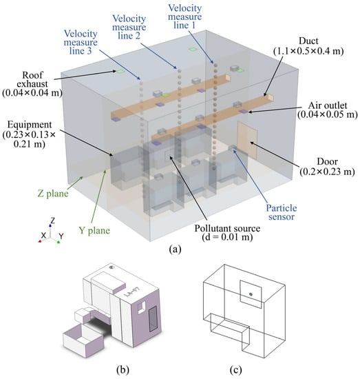
Figure 1.
Schematic view of the factory model: (a) the schematic diagram of the model; (b) the LA-type CNC lathe; (c) the simplified model of the lathe.
The heat was neglected inside the factory model, and the flow was regarded as isothermal. The Reynolds number [42] is used as the dimensionless criterion number and is defined as follows:
where u is the air velocity, m/s; v is the air kinematic viscosity coefficient, m2/s; and d is the characteristic size of the outlet, m.
2.2. Experimental System
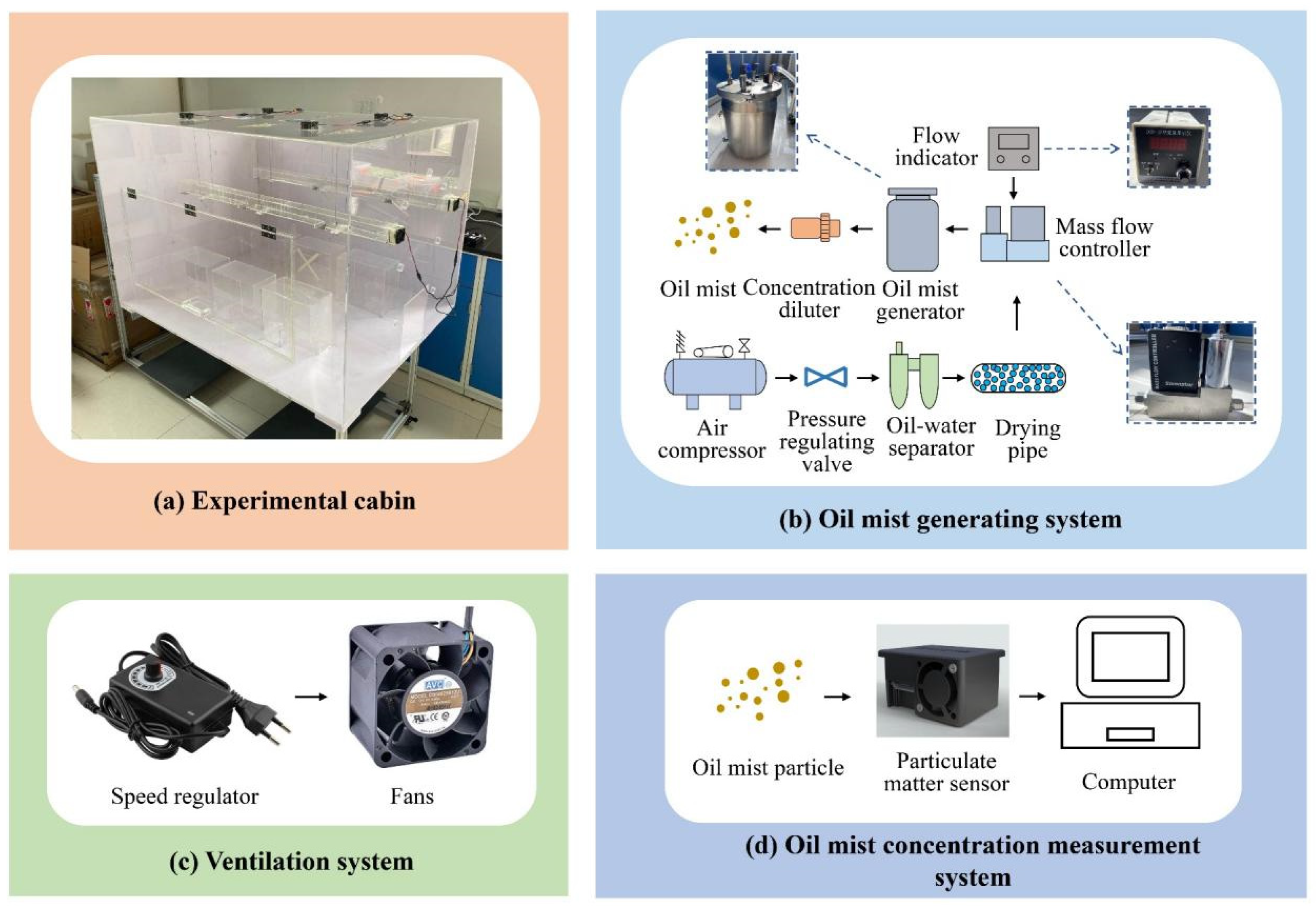
The experimental system is shown in Figure 2, which mainly includes (a) an experimental cabin, (b) an oil mist generating system, (c) a ventilation system, and (d) an oil mist concentration measurement system. In the oil mist generation system, the high-pressure air is generated by the air compressor. The compressed air is treated by the water–oil separator and drying tube and then enters the oil mist generator. The aerosol is released through a nozzle in the generator. To ensure a stable air flow, the compressed air is controlled by a mass flow controller (range: 0 to 50 L/min). A concentration diluter is connected to the outlet of the oil mist generator. By adjusting the value of the mass flow controller, the airflow into the aerosol generator can be controlled at a low flow rate to ensure a stable amount of oil mist emission. The ventilation system consists of a fan and a speed controller. The speed controller changes the fan speed to control the ventilation volume.
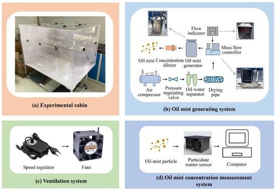
Figure 2.
Experimental system.
Particle concentration in the chamber was measured by a particulate matter (PM) A4-CG PM sensor, which uses a laser light scattering method and has a built-in laser transmitter as well as a photoelectric receiving element. Table 2 shows the parameters of the PM sensors, and Figure 1a shows the measurement positions. In addition, a hot wire anemometer type Testo405i (Testo SE & Co. KGaA, Titisee-Neustadt, Germany) was used to measure air velocity, and the measurement positions are also shown in Figure 1a. Dioctyl sebacate (DOS) was used as the particle type in this research. DOS is a colorless or yellowish-transparent oily liquid that is not volatile and has a density of 913 kg/m3 at 20 °C. It maintained a stable shape and particle size during the experiment.
Table 2.
Parameters of the PM sensor.
2.3. Experimental Procedure and Setup
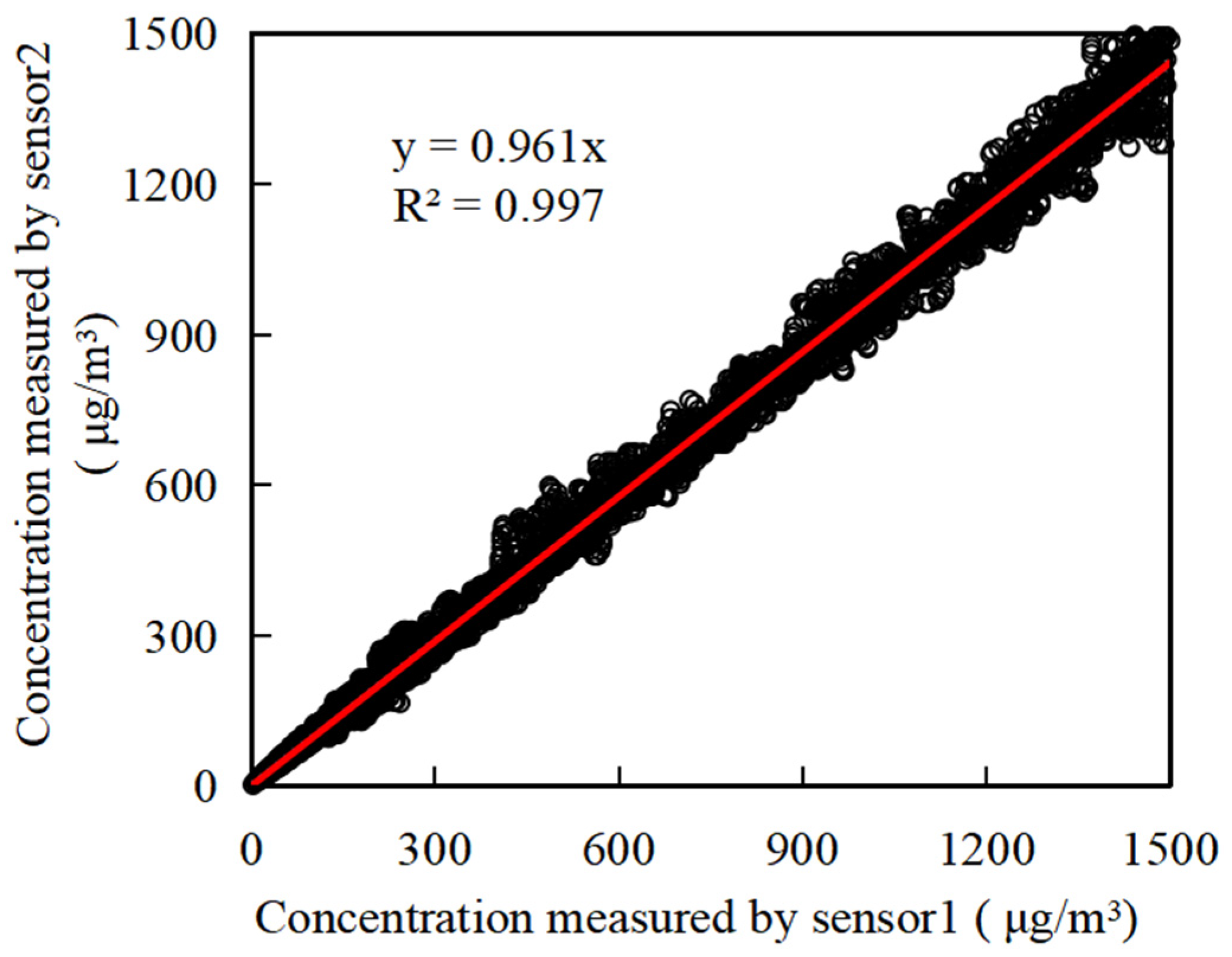
To perform simultaneous multi-point measurements, it is necessary to ensure the consistency of the measurement results from each sensor. During the measurement, the ambient temperature was set at 24 °C and the relative humidity was 20%. The instruments and calibration methods used were consistent with those of Zhang et al. [43]. Sensor 1 was used as a reference to measure the deviation degree of other sensors relative to Sensor 1. Figure 3 shows the comparison of measurement results from Sensors 1 and 2, where 0.961 is the consistency parameter. More measurements are shown in Table 3.
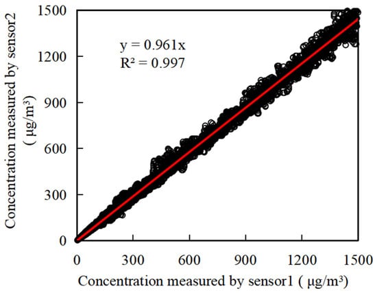
Figure 3.
Measurement consistency of two sensors.
Table 3.
Sensor consistency.
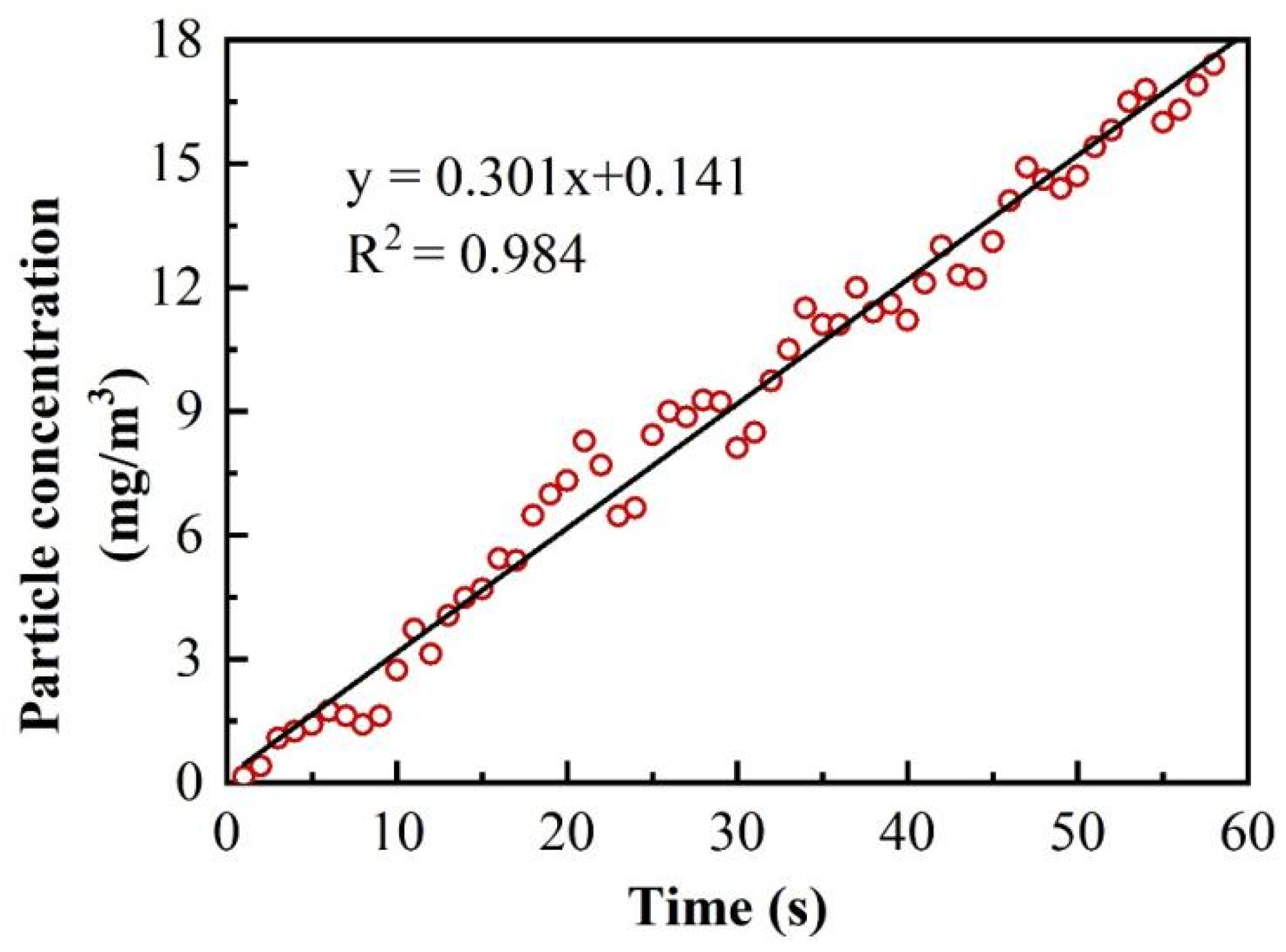
The particle concentration in the room satisfies the following Equation (3). The rate of oil mist emission can be obtained by measuring the corresponding concentration.
where V is the chamber volume, m3; C is particle concentration, mg/m3; and E is the particle emission rate, mg/s. Due to the small particle size and low settling velocity, particle deposition is neglected.
To measure the rate of oil mist emission, an experimental chamber was first closed, and a fan was used for mixing inside to ensure adequate mixing of the particles inside the chamber. Figure 4 shows the emission rate results from Equation (3) and the aerosol detector. The slope of the fitting curve was 0.3, the volume of the test bench was 0.028 m3, and the emission rate was calculated as 0.0085 mg/s. The lathe’s oil mist emission ranges from 0.007 mg/s to 0.114 mg/s.

Figure 4.
Oil mist emission rate.
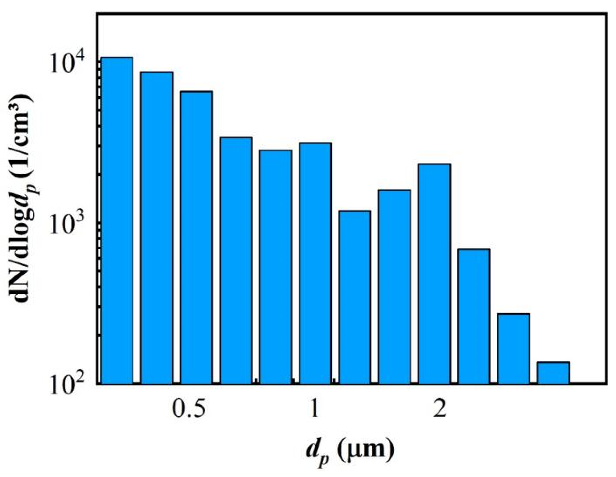
In addition, the particle size distribution was measured by a TSI DustTrak II 8530 aerosol detector at the same rate of oil mist emission, and the results are shown in Figure 5. It shows particle size distribution during emission: roughly less than 1 µm, with a median diameter of 0.5 µm, which is similar to the on-site measurements that the aerodynamic diameters of the oil particles are in the range of 0.5–0.8 µm [1]. The experiments were conducted under roof exhaust and mixed ventilation conditions, both of which are commonly used in factories. Under roof exhaust conditions, the exhaust air velocity is 3.25 m/s, and under mixed ventilation conditions, the exhaust air velocity is 3.75 m/s, and the air supply volume of each air duct is 30 m3/h. During the experiment, the corresponding experimental data were recorded when the whole system reached stability. The air velocity is measured at line 1 (X = 0.3 m, Y = 0.45 m), line 2 (X = 0.6 m, Y = 0.45 m) and line 3 (X = 0.9 m, Y = 0.45 m). The oil mist concentration is measured by 9 sensor located in three vertical lines (line 4: X = 0.3 m, Y = 0.6 m; line 5: X = 0.6 m, Y = 0.6 m; line 6: X = 0.9 m, Y = 0.6 m).

Figure 5.
Particle size distribution of oil mist produced by DOS.
3. Numerical Method
For oil mist transport in a machining factory, the oil volume is usually only a small fraction of the total air volume. Therefore, the effect of oil mist on the flow field is negligible. In this study, the Eulerian–Eulerian (EE) and Eulerian–Lagrangian (EL) models were used to study the distribution of oil mist in the factory.
3.1. Eulerian-Based Flow Model
In this study, the RNG k-ε model was selected to study the airflow and the governing equation can be written in a general form as follows:
where ρ is the fluid density, kg/m3; ui is the fluid velocity, m/s; ϕ is a generalized variable (velocity, temperature, concentration); Γϕ is the diffusion coefficient; and Sϕ is the source term. The parameters of this model are summarized in Table 4.
Table 4.
Coefficients for RNG k-ε model.
3.1.1. Eulerian–Eulerian Model
For the Eulerian–Eulerian method, the particle phase is treated as a continuous phase. The governing equation of convection diffusion was considered as:
where i is the component index, V is the volume, ji is the diffusion flux; a is the area vector; is the velocity, m/s; Sϕi is the source item.
3.1.2. Eulerian–Lagrangian Model
For the Eulerian–Lagrangian model, particles are tracked using the Lagrangian method while airflow is analyzed using Eulerian equations. Particle motion is defined as:
where and are the local air and particle velocity, m/s; μ is air viscosity, kg/(m·s); ρ and ρp and the air and particle density, respectively, kg/m3; dp is the particle diameter, m; Cc is the Cunningham factor; is the gravity acceleration, m/s2; is additional forces acting on the particle.
The includes two components: average velocity and instantaneous velocity. The former is obtained by solving the RANS equations, and the latter needs to be modeled by the discrete random walk (DRW) model. In the DRW model, the interaction of a particle with a fluid-phase turbulent eddy is simulated [44]. The instantaneous velocities follow the Gaussian distribution, and they are correlated with the flow of turbulent kinetic energy and the concentration distribution obtained by the particle trajectories.
where is the instantaneous velocity, ξ is the Gaussian random number, and k is the turbulent kinetic energy.
3.2. Boundary Conditions
The air supply inlet and exhaust outlet were set at constant positive and negative velocities, respectively. The door was set up as a pressure outlet. The wall was considered a no-slip boundary. The deposition velocity of particles (diameter = 0.5 μm) was 1.0 × 10⁻⁵ and the deposition rate was 0.24 h−1, about two orders of magnitude lower than the air exchange rate [45]. Therefore, particle deposition was ignored in Lagrangian and Eulerian models, adopting complete rebound and zero flux (gradient zero condition) at the wall, respectively. Other boundary conditions are shown in Table 5.
Table 5.
CFD boundary settings.
3.3. Grid and Numerical Schemes
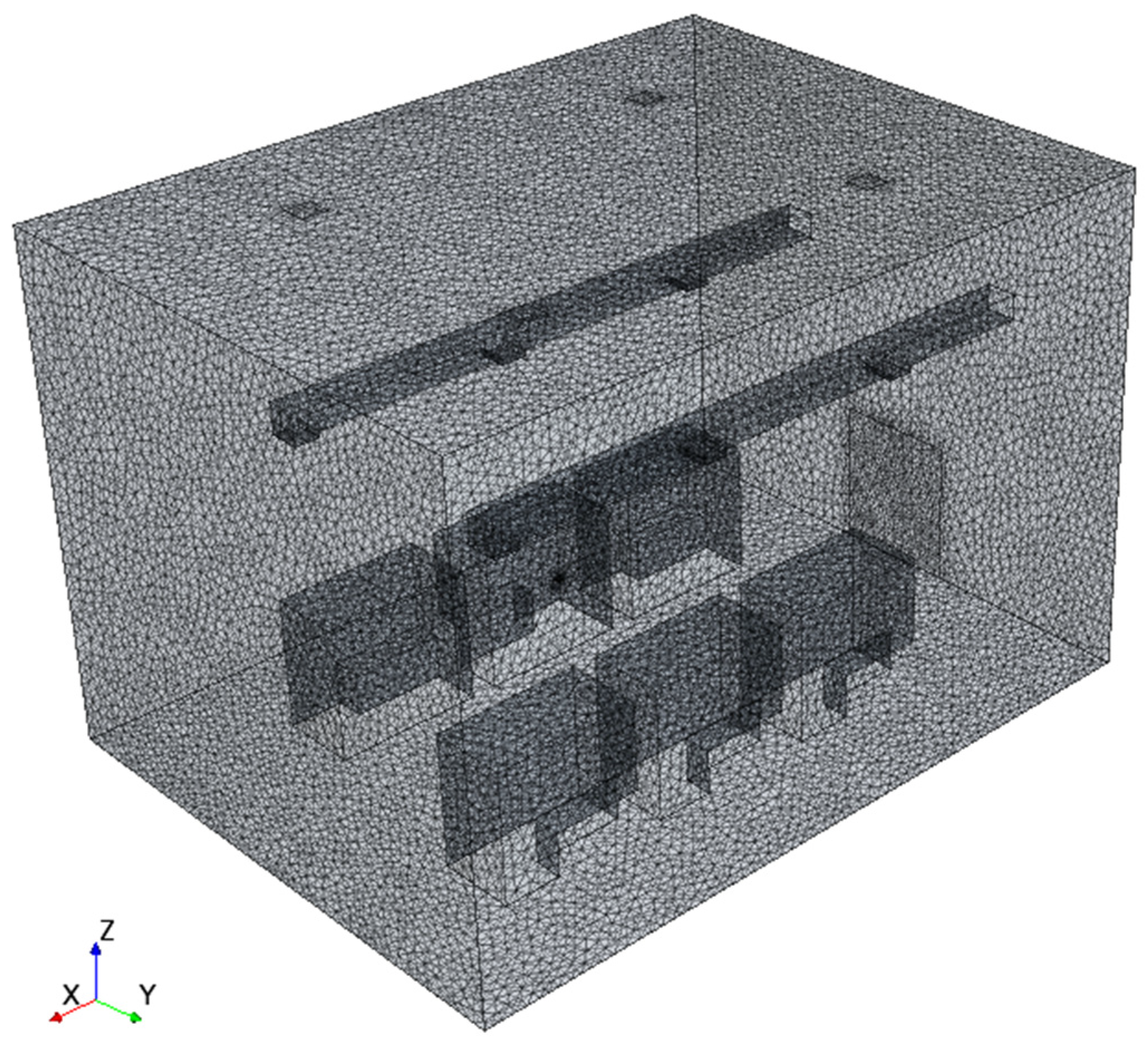
In this study, a tetrahedral grid was used and fine mesh was used for the air inlet and outlet, as shown in Figure 6. The wall function was set as the standard wall function, so the y* was greater than 11.225 [46,47]. The model was divided into different grid numbers, namely, 0.36 million, 0.69 million, 1.43 million, and 2.80 million. The details of the calculations are shown in Section 4. This investigation used the finite volume method to discretize the governing equations and the semi-implicit method for pressure linked equations (SIMPLE) algorithm to couple the pressure and velocity. The pressure staggering option (PRESTO!) scheme was adopted for pressure discretization, and the second-order upwind discretization scheme was used for iterations for all variables except pressure to achieve higher accuracy. Convergence was reached when the residuals were less than 10−6 or air velocity and oil mist concentration varied within a limited range at some monitoring sites. In the Lagrangian model, the quantity concentration of particles below 2.5 μm in the machining workshop is maintained at 400~800 P/cm3 and accounts for more than 98% [2]. Converted to volume fractions, it is approximately 1.4 × 10⁻⁸~2.7 × 10⁻⁸. Since indoor particulate matter usually occupies a very low volume fraction, the effect of airflow on the distribution of oil mist is usually studied, rather than the other way around [48]. Thus, the effect of discrete relatively continuous phases is not considered in this paper, i.e., a single-phase coupling approach is adopted.
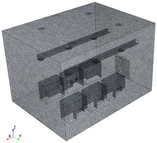
Figure 6.
Schematic diagram of the grid.
3.4. Calculation Error Analysis
In this study, the CFD results were compared with experimental data, and the computational results of different CFD also be compared. This study used dimensionless variables that were defined as Equation (8).
where u is the velocity at the measurement point, m/s; uo is the supply velocity, m/s. Co is the supply concentration, mg/m3; CR is the return concentration, mg/m3. In this study, CR is the concentration at the exhaust outlet. Co is the concentration at the inlet.
The standard deviation was used to express the error, and the errors are calculated as follows:
where σu, σc are the errors of velocity and oil mist concentration, respectively; n is the number of sampled data; and are the average values of velocity and oil mist concentration, respectively; ui and Ci are the results values of velocity and oil mist concentration, respectively.
4. Results
4.1. Flowfield Distribution
4.1.1. Roof Exhaust Condition
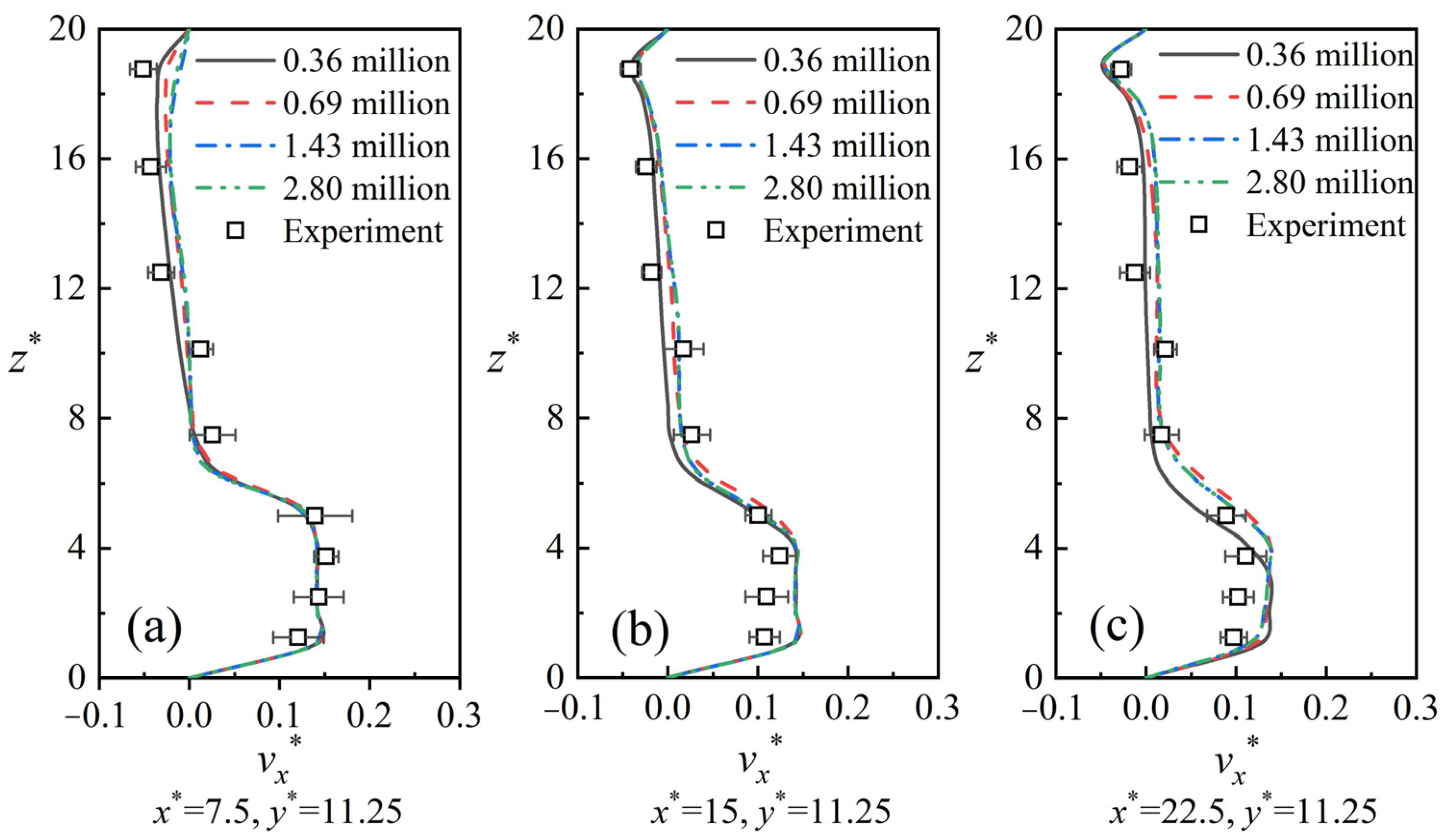
This section compares the simulated and experimental results of air velocity for the roof exhaust condition and measures the computational error for different numbers of grids. Figure 7 shows the comparison of experimental and measured results for different measurement positions with different grid numbers. Table 6 shows the relative errors of the calculation results under different grid numbers.
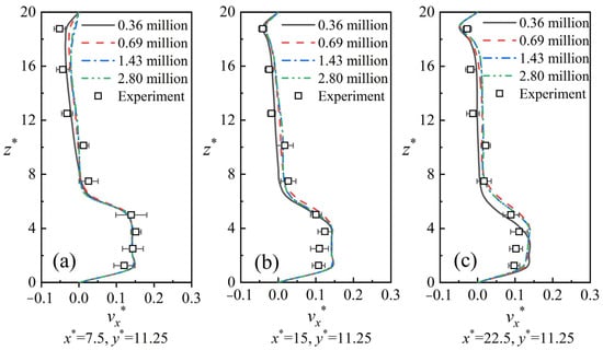
Figure 7.
Comparison of numerical and experimental results under the roof exhaust condition. (a–c) are the comparisons of experimental and CFD results at lines 1, 2 and 3 with different grid numbers.
Table 6.
Computational error of different grid numbers.
From Table 6, it can be found that the computational error on each line is less than 6.74% when the grid number is increased from 1.43 million to 2.80 million, while the computational error on each line is 20–30% when the grid is increased from 0.69 million to 1.43 million. Therefore, this study continues the follow-up study at the grid number of 1.43 million. Figure 7 shows that the experimental data and the simulation results are in good agreement, which also indicates that the numerical model used in this study is feasible.
Figure 8 shows the distribution of the flow field in the exhaust condition of the Z plane (Z = 0.13 m) and Y plane (Y = 0.45 m), which shows that the aisle between the two rows of equipment has high air velocity, and some vortices are distributed inside the factory space, mainly between the equipment and the wall and near the roof. The presence of many vortices in the space and the direction of the airflow is not always towards the exhaust air outlet, which may lead to high pollutant concentrations in the factory.
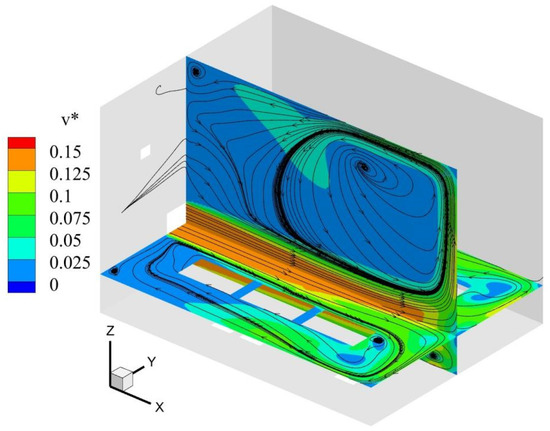
Figure 8.
Flow field under roof exhaust conditions.
4.1.2. Mixed Ventilation Conditions
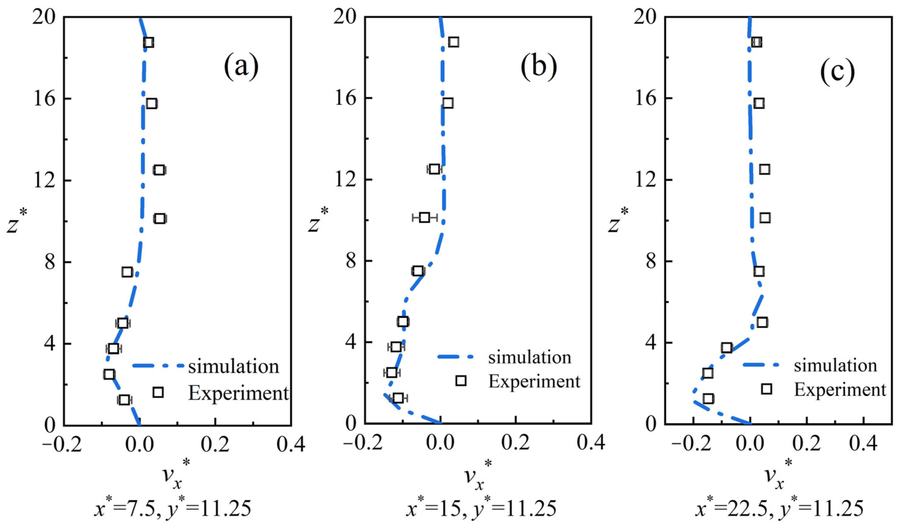
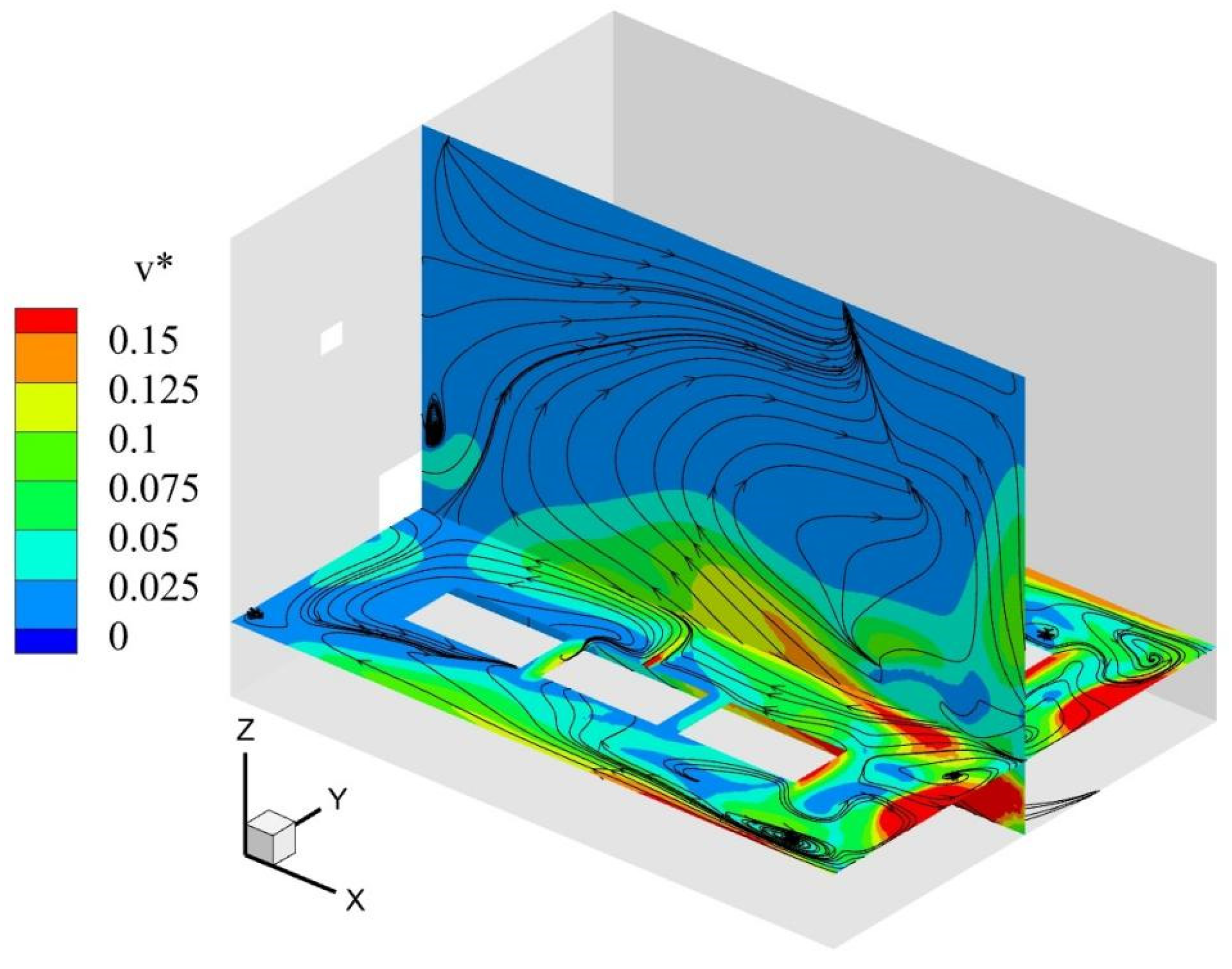
Referring to the results in the previous section, this section uses the same grid strategy for the calculation of the flow field under mixed ventilation conditions. Figure 9 shows the comparison of experimental and measured results in mixed ventilation conditions. Figure 10 shows the distribution of the flow field in mixed ventilation conditions. From Figure 9, it can be seen that the numerical results are more consistent with the experimental results at lower altitudes. When the altitude increases, the difference between the experimental and numerical results is greater due to the smaller airflow velocity. In general, the experimental and numerical results are in agreement. Figure 10 shows that due to the influence of the ducted air supply system, there are fewer vortices in the room compared to when only the roof exhaust is available. While there is more airflow directed to the roof vents, the higher airflow velocity is more concentrated in the lower part of the factory, which may lead to excessive concentrations of pollutants in certain parts.
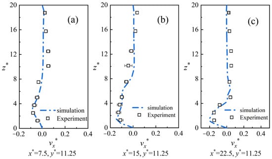
Figure 9.
Comparison of numerical and experimental results under mixed ventilation conditions. (a–c) are the comparisons of experimental and CFD results at lines 1, 2 and 3.
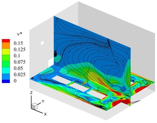
Figure 10.
Flow field under mixed ventilation conditions.
4.2. Particle Transport under Roof Exhaust Ventilation
In this section, indoor pollutant transport under roof exhaust conditions is investigated, and the results of the Eulerian and Lagrangian methods are compared.
4.2.1. Quality Control of the Lagrangian Method
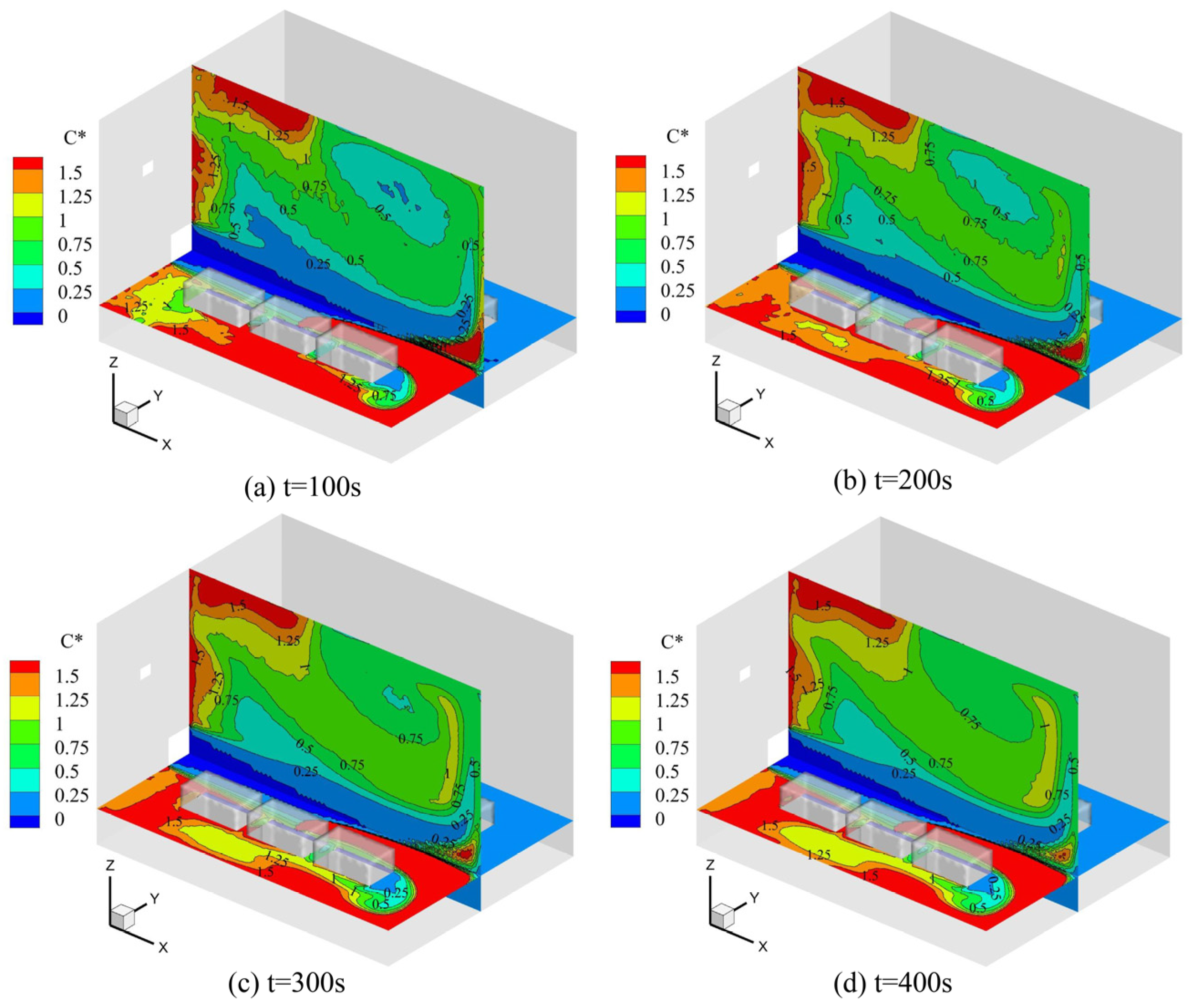
Many factors affect the calculation results of the Lagrangian method, among which the most obvious influence is the calculation time. Therefore, this section first investigates the concentration distributions at different calculation times. Figure 11 shows the concentration distribution at different calculation times. It can be found that when the calculation time is short, such as t = 100 s, the spatial concentration distribution is not continuous, and as time increases, the concentration distribution gradually becomes continuous. Moreover, the change in particle concentration distribution from t = 300 s to t = 400 s is not obvious.

Figure 11.
Oil mist concentration distribution at different times under roof exhaust conditions.
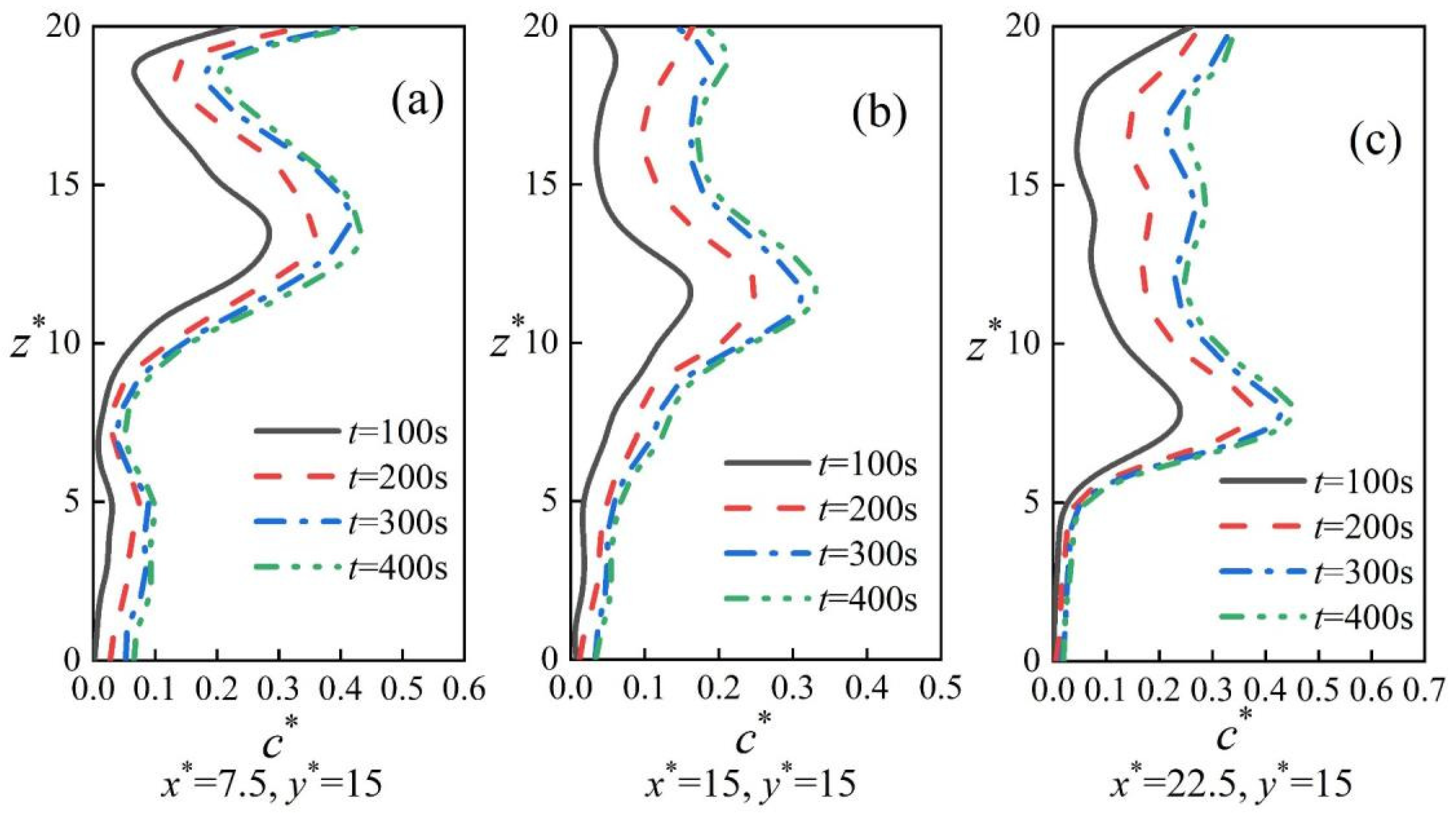
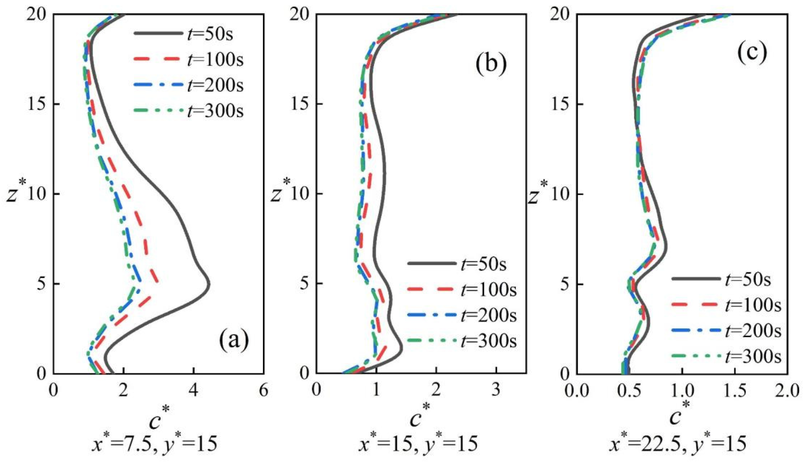
Figure 12 shows the oil mist concentration on the monitoring line at different times, and it can be found that the oil mist concentration rises as time increases. When the time increases from t = 300 s to t = 400 s, the pollutant concentration changes are no longer obvious. The average calculation error of t = 100 s and t = 300 s is about 200%, while the average error of t = 300 s and t = 400 s is less than 10%. Considering the computation time, for a computer with a 128-core CPU, the computation time for t = 100 s, t = 200 s, t = 300 s, and t = 400 s is 2 h, 7.5 h, 15 h, and 25 h, respectively, provided that the boundary conditions are consistent. Therefore, t = 300 s was chosen as the final result.
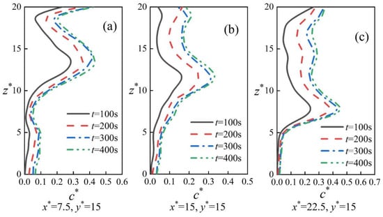
Figure 12.
Oil mist concentrations at different times under roof exhaust conditions on different lines. (a–c) are the comparisons of CFD results with different computation times at the sensor positions of lines 4, 5 and 6.
4.2.2. Comparison of Eulerian and Lagrangian Calculation Results
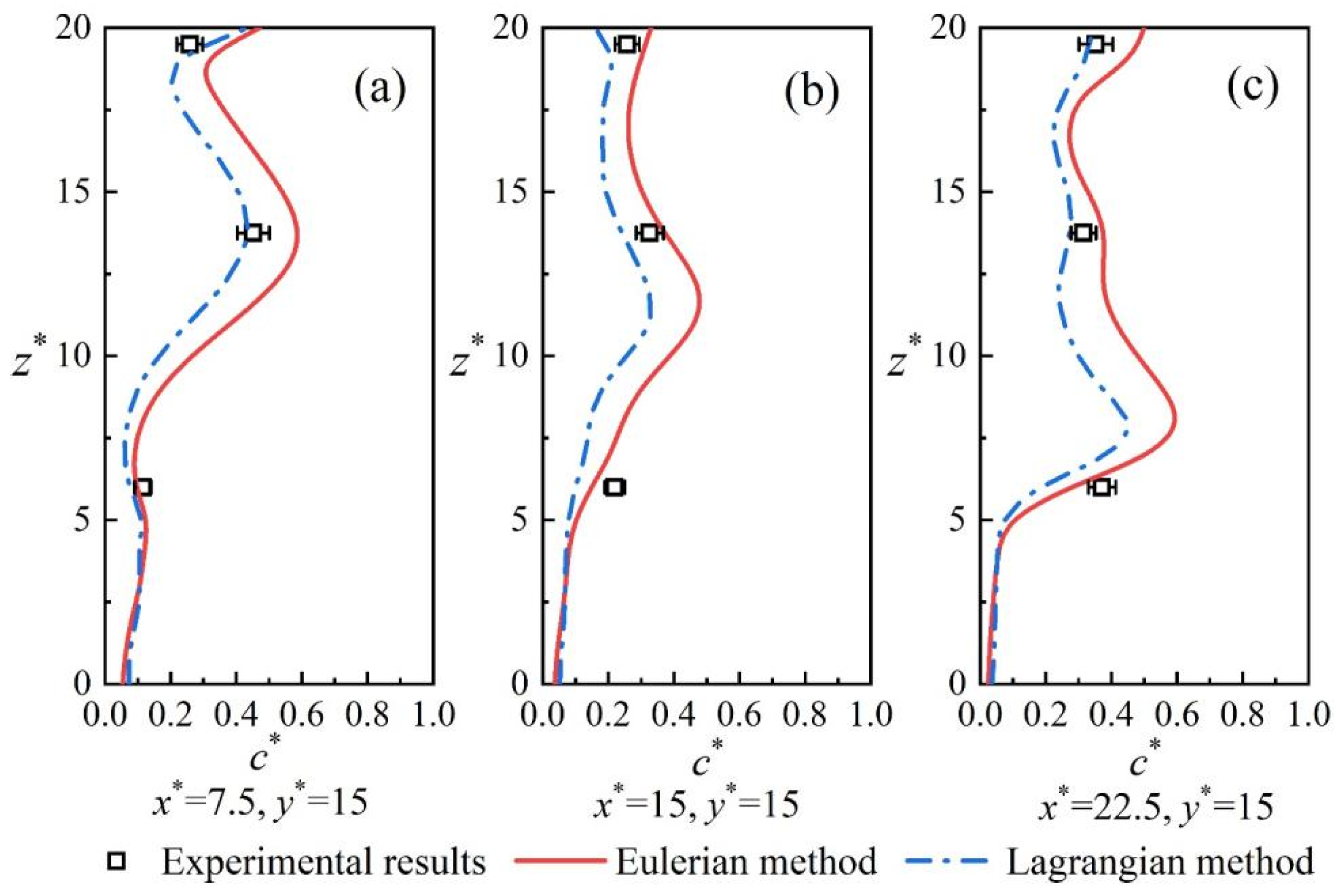
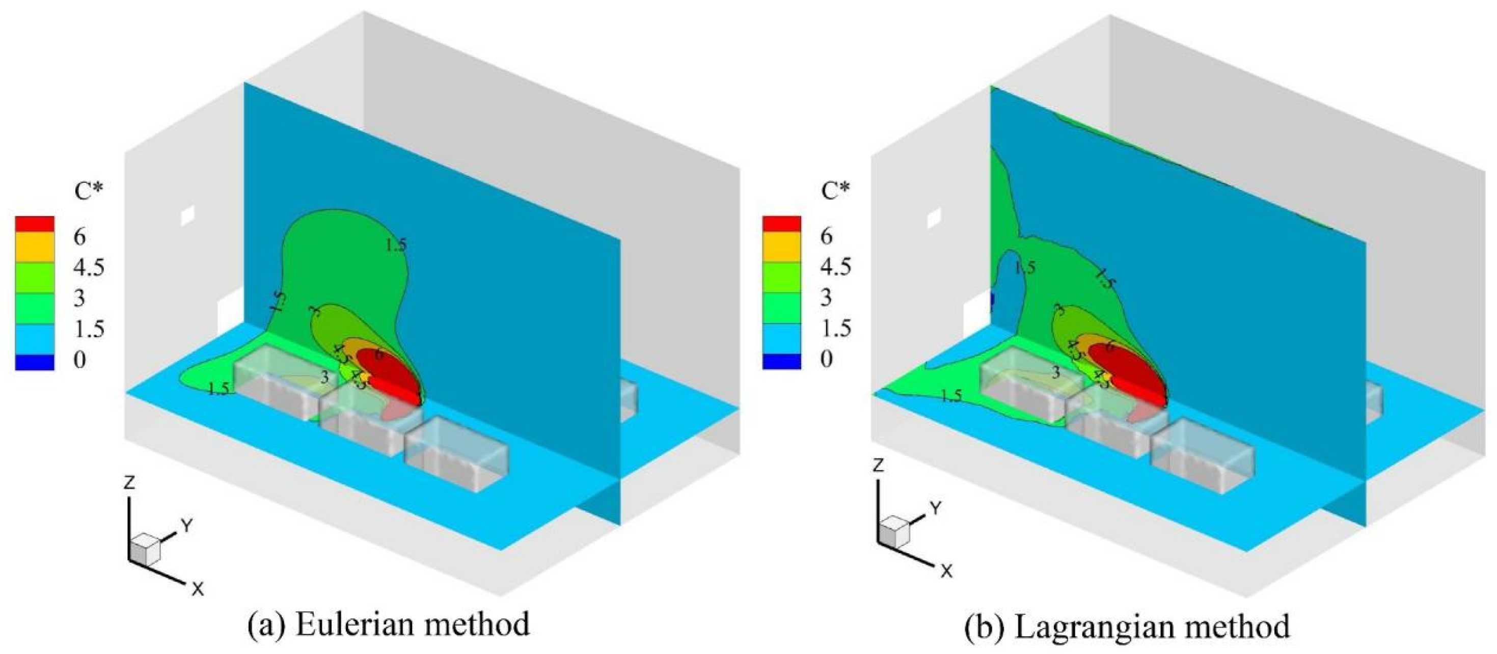
Figure 13 shows the distribution of oil mist concentration calculated by different methods, where Figure 13a,b are the results of the Eulerian and Lagrangian methods, respectively. Combined with the flow field shown in Figure 8, it can be found that the Lagrangian result has a higher oil mist concentration near the vortex at the wall, while the Eulerian method shows a stronger “diffusion effect”. In general, the difference between the two concentration distributions is not significant. Figure 14 shows the simulation results of the Eulerian and Lagrangian methods compared with the experimental results at different locations. The average error of the two methods is about 20%, and the two methods’ results are acceptable compared with the experimental results.
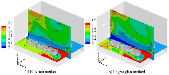
Figure 13.
Oil mist concentration distribution of different methods under roof exhaust conditions.
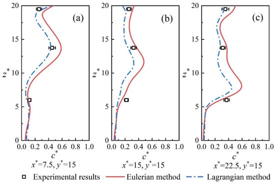
Figure 14.
Comparison of experimental and simulation results of oil mist concentration under roof exhaust conditions. (a–c) are the comparisons of experimental and CFD results at the sensor positions of lines 4, 5 and 6.
4.3. Particle Transport under Mixed Ventilation
4.3.1. Quality Control of the Lagrangian Method
The difference between the flow fields under mixed ventilation and roof exhaust is large. To obtain more accurate Lagrangian calculation results, the calculated oil mist concentration at different times is compared under mixed ventilation conditions. Figure 15 shows the distribution of oil mist concentration at different times. Different from the roof exhaust conditions, the space reaches stability faster at a greater distance from the pollution source because there are fewer vortices in the room, which reduces the residence time of particles in the space. Figure 16 shows the simulation results of the Eulerian and Lagrangian methods compared with the experimental results at different locations. From the figure, it can be found that the average error of t = 50 s and t = 200 s is about 20%, and the average error of t = 200 s and t = 300 s is less than 5%. In addition, t = 100 s, t = 200 s, and t = 300 s took 2 h, 7 h, and 14.5 h, respectively, on a computer with the same 128-core CPU. Therefore, t = 200 s was chosen as the calculation time for the Lagrangian method.
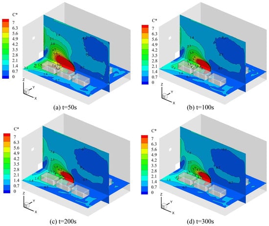
Figure 15.
Oil mist concentration distribution of different methods under mixed ventilation conditions.
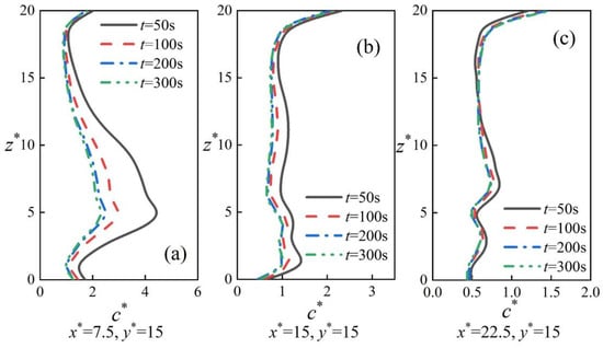
Figure 16.
Oil mist concentrations at different times under mixed ventilation conditions on different lines. (a–c) are the comparisons of CFD results with different computation times at the sensor positions of lines 4, 5 and 6.
4.3.2. Comparison of Eulerian and Lagrangian Calculation Results
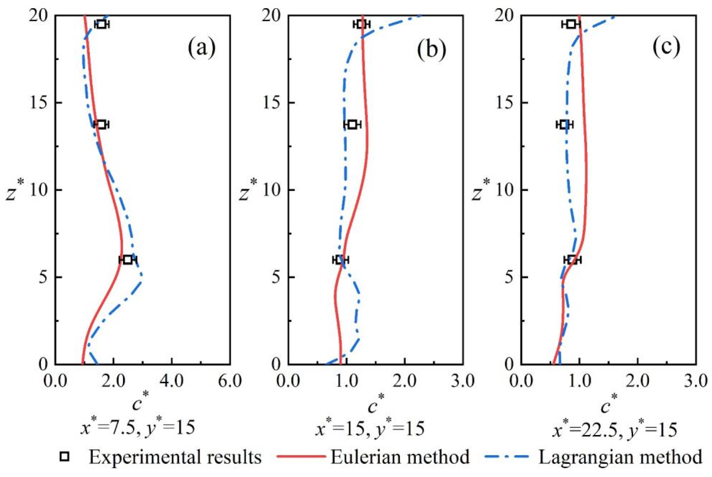
Figure 17 shows the oil mist concentration distributions calculated by different methods under mixed ventilation conditions, where Figure 17a and Figure 18b show the results of the Eulerian and Lagrangian methods, respectively. The differences between these two concentration distributions are mainly concentrated in the position near the roof. According to the flow field in Figure 10, it can be seen that although most of the flow lines are toward the roof, some of them flow near the left wall. Where there is a vortex that causes the particles to collide with the wall several times and reduce the total distance traveled in the Lagrangian model, the Eulerian method does not have the same problem. Figure 17a,b show similar conclusions, with the Lagrangian method calculating higher concentrations near the left wall, while the Eulerian method has higher concentrations in the upper part near the roof. Figure 18 shows the comparison between the calculation results of the Eulerian method and the Lagrangian method with the experiment. The average error of the calculation of the two methods is about 10%, and both methods can better match the concentration trend compared with the experimental results.

Figure 17.
Oil mist concentration distribution of different methods under mixed ventilation conditions ((a,b) are the results of the Eulerian and Lagrangian methods, respectively).
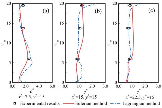
Figure 18.
Comparison of experimental and simulation results of oil mist concentration under mixed ventilation conditions. (a–c) are the comparisons of experimental and CFD results at the sensor positions of lines 4, 5 and 6.
5. Discussion
The calculation of the Lagrangian method needs to consider a variety of factors to ensure the accuracy of the calculation, among which the calculation time has the greatest impact. From the above calculation results, it can be found that the calculation error of oil mist concentration is about 200% for t = 100 s and t = 300 s and less than 10% for t = 300 s and t = 400 s under roof exhaust conditions. Under mixed ventilation conditions, the calculation error is about 20% for t = 50 s and t = 200 s, and the calculation error of oil mist concentration is about 5% for t = 200 s and t = 300 s. This may be because the flow field in roof exhaust conditions in this study is more complex and there are many vortices in the space, resulting in a more difficult diffusion of particulate matter, therefore more time is needed to reach the steady state. In addition, the errors in the calculation of oil mist concentration were 20% and 10% for the Eulerian and Lagrangian methods for roof exhaust conditions and mixed ventilation conditions, respectively. This is due to the presence of more vortices under roof exhaust conditions in this study, which makes it more difficult for the particles to disperse. Indoor oil mist concentration calculations using the Lagrangian method can take longer when the factory flow field environment is more complex and has more vortices than a simple flow field.
For the roof exhaust and mixed ventilation conditions, oil mist concentrations were calculated using the Eulerian and Lagrangian methods based on the same flow field results. Using the same computer, with a 128-core CPU, the calculation time for the Eulerian method is about 1 min for the roof vent conditions, while the Lagrangian method takes 7.5 h. In the mixed ventilation case, the calculation time of the Eulerian method is also about 1 min, while that of the Lagrangian method is 7 h. Overall, the Lagrangian method consumes about 400 times more computational resources than the Eulerian method. Therefore, when simulating oil mist pollutants in industrial factories, the Eulerian method needs to be considered in the first place. In addition, the factory model in this paper is an ideal simplified model with a small volume, and the difference in resource consumption and calculation error between the Eulerian and Lagrangian methods may further increase when calculating the oil mist in a real industrial factory.
In this study, only isothermal conditions were considered. In future studies, humidity should also be included in the particle transport analysis. For particles with an aerodynamic diameter of 0.5 µm, the effects of Brownian diffusion and gravitational settling are relatively small, so a “passive scalar” can be assumed. For particles significantly deviating from this aerodynamic diameter, it is fundamental to model the various forces acting anisotropically on particles. Furthermore, the scalar transport equation for the Eulerian method has not been sufficiently discussed and should be further studied.
6. Conclusions
In this study, a scaled experimental chamber of an industrial factory was built and oil mist dispersion experiments under roof exhaust and mixed ventilation conditions were conducted. Afterward, the oil mist concentration distribution in the factory was calculated using the Eulerian and Lagrangian methods under the same working conditions, and the corresponding calculation errors and resource consumption were compared. This study can provide a reference for the numerical simulation of oil mist concentration in the industrial factory. The main conclusions of the study are as follows.
For oil mist particles with an aerodynamic diameter of 0.5 μm, both Eulerian and Lagrangian methods have a reliable accuracy.
The simulation results of Eulerian and Lagrangian methods for oil mist distribution under mixed ventilation and roof exhaust systems are consistent with the experimental results. The error of the results between the Eulerian and the Lagrangian methods under different conditions is about 10–20%.
When there are more vortices in the factory, the Lagrangian method increases the computation time by more than 53% to satisfy the computational accuracy, and the computational error between the Eulerian and Lagrangian methods becomes about 10% larger.
Based on the same flow field, the Lagrangian method consumes more than 400 times more computational resources than the Eulerian method.
Author Contributions
Conceptualization, S.-J.Y., K.I. and Z.L.; data curation, Y.W.; funding acquisition, Z.L.; investigation, Y.W.; methodology, Y.W., J.S., A.M., S.-J.Y., K.I. and Z.L.; project administration, K.I. and Z.L.; software, Y.W. and J.S.; supervision, Z.L.; validation, Y.W.; visualization, Y.W. and J.S.; writing—original draft, Y.W. and J.S.; writing—review & editing, Y.W., M.Z., A.M., S.-J.Y., K.I. and Z.L. All authors have read and agreed to the published version of the manuscript.
Funding
This work was supported by the National Nature Science Foundation of China (Grant No.51878442).
Data Availability Statement
Not applicable.
Conflicts of Interest
Data from the present research effort are available upon request.
References
- Zhang, J.; Long, Z.; Liu, W.; Chen, Q. Strategy for Studying Ventilation Performance in Factories. Aerosol Air Qual. Res. 2016, 16, 442–452. [Google Scholar] [CrossRef]
- Wang, X.; Zhou, Y.; Wang, F.; Jiang, X.; Yang, Y. Exposure Levels of Oil Mist Particles under Different Ventilation Strategies in Industrial Workshops. Build. Environ. 2021, 206, 108264. [Google Scholar] [CrossRef]
- Yue, Y.; Sun, J.; Gunter, K.L.; Michalek, D.J.; Sutherland, J.W. Character and Behavior of Mist Generated by Application of Cutting Fluid to a Rotating Cylindrical Workpiece, Part 1: Model Development. J. Manuf. Sci. Eng. Trans. ASME 2004, 126, 417–425. [Google Scholar] [CrossRef]
- Chen, M.R.; Tsai, P.J.; Chang, C.C.; Shih, T.S.; Lee, W.J.; Liao, P.C. Particle Size Distributions of Oil Mists in Workplace Atmospheres and Their Exposure Concentrations to Workers in a Fastener Manufacturing Industry. J. Hazard. Mater. 2007, 146, 393–398. [Google Scholar] [CrossRef]
- Lai, C.H.; Chen, Y.C.; Lin, K.Y.A.; Lin, Y.X.; Lee, T.H.; Lin, C.H. Adverse Pulmonary Impacts of Environmental Concentrations of Oil Mist Particulate Matter in Normal Human Bronchial Epithelial Cell. Sci. Total Environ. 2022, 809, 151119. [Google Scholar] [CrossRef]
- Lin, C.H.; Lai, C.H.; Hsieh, T.H.; Tsai, C.Y. Source Apportionment and Health Effects of Particle-Bound Metals in PM2.5 near a Precision Metal Machining Factory. Air Qual. Atmos. Health 2022, 15, 605–617. [Google Scholar] [CrossRef]
- Wang, Y.; Long, Z.; Zhang, H.; Shen, X.; Yu, T. Optimization Study of Sampling Device for Semi-Volatile Oil Mist in the Industrial Workshop. Atmosphere 2022, 13, 1048. [Google Scholar] [CrossRef]
- Piacitelli, G.M.; Sieber, W.K.; O’Brien, D.M.; Hughes, R.T.; Glaser, R.A.; Catalano, J.D. Metalworking Fluid Exposures in Small Machine Shops: An Overview. Am. Ind. Hyg. Assoc. J. 2001, 62, 356–370. [Google Scholar] [CrossRef]
- Park, D.; Stewart, P.A.; Coble, J.B. A Comprehensive Review of the Literature on Exposure to Metalworking Fluids. J. Occup. Environ. Hyg. 2009, 6, 530–541. [Google Scholar] [CrossRef]
- Murga, A.; Yoo, S.J.; Ito, K. Multi-Stage Downscaling Procedure to Analyse the Impact of Exposure Concentration in a Factory on a Specific Worker through Computational Fluid Dynamics Modelling. Indoor Built Environ. 2018, 27, 486–498. [Google Scholar] [CrossRef]
- Ren, J.; Wang, Y.; Liu, Q.; Liu, Y. Numerical Study of Three Ventilation Strategies in a Prefabricated COVID-19 Inpatient Ward. Build. Environ. 2021, 188, 107467. [Google Scholar] [CrossRef] [PubMed]
- Goodson, M.; Feaster, J.; Jones, A.; McGowan, G.; Agricola, L.; Timms, W.; Uddin, M. Modeling Transport of SARS-CoV-2 inside a Charlotte Area Transit System (CATS) Bus. Fluids 2022, 7, 80. [Google Scholar] [CrossRef]
- Zhang, M.; Shrestha, P.; Liu, X.; Turnaoglu, T.; DeGraw, J.; Schafer, D.; Love, N. Computational Fluid Dynamics Simulation of SARS-CoV-2 Aerosol Dispersion inside a Grocery Store. Build. Environ. 2022, 209, 108652. [Google Scholar] [CrossRef] [PubMed]
- Sarhan, A.A.R.; Naser, P.; Naser, J. Aerodynamic Prediction of Time Duration to Becoming Infected with Coronavirus in a Public Place. Fluids 2022, 7, 176. [Google Scholar] [CrossRef]
- López-Rebollar, B.M.; Díaz-Delgado, C.; Posadas-Bejarano, A.; García-Pulido, D.; Torres-Maya, A. Proposal of a Mask and Its Performance Analysis with Cfd for an Enhanced Aerodynamic Geometry That Facilitates Filtering and Breathing against Covid-19. Fluids 2021, 6, 408. [Google Scholar] [CrossRef]
- Mirzaei, P.A.; Moshfeghi, M.; Motamedi, H.; Sheikhnejad, Y.; Bordbar, H. A Simplified Tempo-Spatial Model to Predict Airborne Pathogen Release Risk in Enclosed Spaces: An Eulerian-Lagrangian CFD Approach. Build. Environ. 2022, 207, 108428. [Google Scholar] [CrossRef]
- Murakami, S.; Kato, S.; Nagano, S.; Tanaka, Y. Diffusion Characteristics of Airborne Particles with Gravitational Settling in a Convection-Dominant Indoor Flow Field. ASHRAE Trans. 1992, 98, 82–97. [Google Scholar]
- Lai, A.C.K.; Chen, F.Z. Comparison of a New Eulerian Model with a Modified Lagrangian Approach for Particle Distribution and Deposition Indoors. Atmos. Environ. 2007, 41, 5249–5256. [Google Scholar] [CrossRef]
- Zhao, B.; Yang, C.; Yang, X.; Liu, S. Particle Dispersion and Deposition in Ventilated Rooms: Testing and Evaluation of Different Eulerian and Lagrangian Models. Build. Environ. 2008, 43, 388–397. [Google Scholar] [CrossRef]
- Yan, Y.; Li, X.; Ito, K. Numerical Investigation of Indoor Particulate Contaminant Transport Using the Eulerian-Eulerian and Eulerian-Lagrangian Two-Phase Flow Models. Exp. Comput. Multiph. Flow 2020, 2, 31–40. [Google Scholar] [CrossRef]
- Gao, N.P.; Niu, J.L. Modeling Particle Dispersion and Deposition in Indoor Environments. Atmos. Environ. 2007, 41, 3862–3876. [Google Scholar] [CrossRef]
- Zhao, B.; Zhang, Z.; Li, X.; Huang, D. Comparison of Diffusion Characteristics of Aerosol Particles in Different Ventilated Rooms by Numerical Method. In Proceedings of the Ashrae 2004 Winter Meeting, Anaheim, CA, USA, 24–28 January 2004; pp. 89–96. [Google Scholar]
- Zhang, Z.; Chen, Q. Comparison of the Eulerian and Lagrangian Methods for Predicting Particle Transport in Enclosed Spaces. Atmos. Environ. 2007, 41, 5236–5248. [Google Scholar] [CrossRef]
- Tang, Y.; Guo, B. Computational Fluid Dynamics Simulation of Aerosol Transport and Deposition. Front. Environ. Sci. Eng. China 2011, 5, 362–377. [Google Scholar] [CrossRef]
- Li, X.; Yan, Y.; Shang, Y.; Tu, J. An Eulerian-Eulerian Model for Particulate Matter Transport in Indoor Spaces. Build. Environ. 2015, 86, 191–202. [Google Scholar] [CrossRef]
- Wang, M.; Lin, C.H.; Chen, Q. Advanced Turbulence Models for Predicting Particle Transport in Enclosed Environments. Build. Environ. 2012, 47, 40–49. [Google Scholar] [CrossRef]
- Chen, C.; Liu, W.; Lin, C.H.; Chen, Q. Comparing the Markov Chain Model with the Eulerian and Lagrangian Models for Indoor Transient Particle Transport Simulations. Aerosol Sci. Technol. 2015, 49, 857–871. [Google Scholar] [CrossRef]
- Xu, Z.; Han, Z.; Qu, H. Comparison between Lagrangian and Eulerian Approaches for Prediction of Particle Deposition in Turbulent Flows. Powder Technol. 2020, 360, 141–150. [Google Scholar] [CrossRef]
- Wei, G.; Chen, B.; Lai, D.; Chen, Q. An Improved Displacement Ventilation System for a Machining Plant. Atmos. Environ. 2020, 228, 117419. [Google Scholar] [CrossRef]
- Chen, F.; Yu, S.C.M.; Lai, A.C.K. Modeling Particle Distribution and Deposition in Indoor Environments with a New Drift-Flux Model. Atmos. Environ. 2006, 40, 357–367. [Google Scholar] [CrossRef]
- Zhao, B.; Chen, C.; Tan, Z. Modeling of Ultrafine Particle Dispersion in Indoor Environments with an Improved Drift Flux Model. J. Aerosol Sci. 2009, 40, 29–43. [Google Scholar] [CrossRef]
- Zhang, Z.; Chen, Q. Prediction of Particle Deposition onto Indoor Surfaces by CFD with a Modified Lagrangian Method. Atmos. Environ. 2009, 43, 319–328. [Google Scholar] [CrossRef]
- Zhang, Z.; Chen, Q. Experimental Measurements and Numerical Simulations of Particle Transport and Distribution in Ventilated Rooms. Atmos. Environ. 2006, 40, 3396–3408. [Google Scholar] [CrossRef]
- Cao, Q.; Liu, M.; Li, X.; Lin, C.H.; Wei, D.; Ji, S.; Zhang, T.; Chen, Q. Influencing Factors in the Simulation of Airflow and Particle Transportation in Aircraft Cabins by CFD. Build. Environ. 2022, 207, 108413. [Google Scholar] [CrossRef] [PubMed]
- Cao, Z.; Bai, Y.; Wang, Y.; An, Y.; Zhang, C.; Zhao, T.; Zhai, C.; Lv, W.; Zhou, Y.; Wu, S. Numerical Study on the Effect of Buoyancy-Driven Pollution Source on Vortex Ventilation Performance. Build. Environ. 2022, 225, 109634. [Google Scholar] [CrossRef]
- Wei, X.; Yi, D.; Xie, W.; Gao, J.; Lv, L. Protection against Inhalation of Gaseous Contaminants in Industrial Environments by a Personalized Air Curtain. Build. Environ. 2021, 206, 108343. [Google Scholar] [CrossRef]
- Huang, Y.; Guo, S.; Gao, H.; Wang, Y.; Li, W.; Zhang, Y.; Wang, Z. Flow-Field Characteristics and Ventilation Performance of the High-Temperature Buoyant Jet Controlled by Spray-Local Exhaust Ventilation. Build. Environ. 2022, 225, 109644. [Google Scholar] [CrossRef]
- Wang, Y.; Cao, Y.; Liu, B.; Liu, J.; Yang, Y.; Yu, Q. An Evaluation Index for the Control Effect of the Local Ventilation Systems on Indoor Air Quality in Industrial Buildings. Build. Simul. 2016, 9, 669–676. [Google Scholar] [CrossRef]
- Yang, Y.; Zhang, Y.; Liu, F.; Wang, Y.; Cao, Q.; Fan, J.N.; Zhang, Y.; Chen, H. Distribution and Removal Efficiency of Sulfuric Droplets under Two General Ventilation Modes. Build. Environ. 2022, 207, 108563. [Google Scholar] [CrossRef]
- Wang, Y.; Guo, Y.; Hao, W.; Liu, W.; Long, Z. Simulation Study of the Purification System for Indoor Oil Mist Control in Machining Factories. Build. Simul. 2023, 16, 1361–1374. [Google Scholar] [CrossRef]
- Wang, Y.; Shen, X.; Yoo, S.J.; Long, Z.; Ito, K. Error Analysis of Human Inhalation Exposure Simulation in Industrial Workshop. Build. Environ. 2022, 224, 109573. [Google Scholar] [CrossRef]
- Posner, J.D.; Buchanan, C.R.; Dunn-Rankin, D. Measurement and Prediction of Indoor Air Flow in a Model Room. Energy Build. 2003, 35, 515–526. [Google Scholar] [CrossRef]
- Zhang, H.; Zhang, S.; Pan, W.; Long, Z. Low-Cost Sensor System for Monitoring the Oil Mist Concentration in a Workshop. Environ. Sci. Pollut. Res. 2021, 28, 14943–14956. [Google Scholar] [CrossRef] [PubMed]
- ANSYS, F. ANSYS Fluent Theory Guide 19.1.; ANSYS: Canonsburg, PA, USA, 2019. [Google Scholar]
- Lai, A.C.K.; Nazaroff, W.W. Modeling Indoor Particle Deposition from Turbulent Flow onto Smooth Surfaces. J. Aerosol Sci. 2000, 31, 463–476. [Google Scholar] [CrossRef]
- Aliabadi, A.A.; Veriotes, N.; Pedro, G. A Very Large-Eddy Simulation (VLES) Model for the Investigation of the Neutral Atmospheric Boundary Layer. J. Wind Eng. Ind. Aerodyn. 2018, 183, 152–171. [Google Scholar] [CrossRef]
- Wen, S.; Liu, J.; Zhang, F.; Xu, J. Numerical and Experimental Study towards a Novel Torque Damper with Minimized Air Flow Instability. Build. Environ. 2022, 217, 109114. [Google Scholar] [CrossRef]
- Holmberg, S.; Li, Y. Modelling of the indoor environment–particle dispersion and deposition. Indoor Air 1998, 8, 113–122. [Google Scholar] [CrossRef]


Disclaimer/Publisher’s Note: The statements, opinions and data contained in all publications are solely those of the individual author(s) and contributor(s) and not of MDPI and/or the editor(s). MDPI and/or the editor(s) disclaim responsibility for any injury to people or property resulting from any ideas, methods, instructions or products referred to in the content. |
© 2023 by the authors. Licensee MDPI, Basel, Switzerland. This article is an open access article distributed under the terms and conditions of the Creative Commons Attribution (CC BY) license (https://creativecommons.org/licenses/by/4.0/).