Article

Engine Mass Flow Estimation through Neural Network Modeling in Semi-Transient Conditions: A New Calibration Approach

1
Atris Engineering srl, 41122 Modena, Italy
2
Paul G. Allen School of Computer Science and Engineering, University of Washington, Seattle, WA 98195, USA
3
Motori Minarelli spa, 40012 Calderara di Reno, Italy
4
Department of Engineering “Enzo Ferrari”, University of Modena and Reggio Emilia, 42121 Reggio Emilia, Italy
*
Author to whom correspondence should be addressed.
Fluids 2024, 9(10), 239; https://doi.org/10.3390/fluids9100239
Submission received: 4 September 2024 / Revised: 7 October 2024 / Accepted: 8 October 2024 / Published: 12 October 2024
(This article belongs to the Special Issue Machine Learning and Artificial Intelligence in Fluid Mechanics)

Abstract

:
Nowadays, engine experimental research represents a very expensive field within the automotive industry, but it remains fundamental for engine and vehicle development. The present work aims to investigate a novel approach for engine control system calibration, by adopting machine learning techniques to model physical parameters of the engine starting from experimental data measured at the test bench. The main goal is to create a methodology which accelerates the calibration process without losing accuracy. A model that estimates air mass flow is created by adopting either a tree ensemble model or an artificial neural network trained on a small dataset, which was previously acquired at the test bench using a random calibration of the volumetric efficiency map. The model’s performance is first validated on a larger, random dataset. Then, the volumetric efficiency calculated from the air mass flow model estimation is used to calibrate the transfer function of the Engine Control Unit. Finally, the sensitivity of the model error correlated with the number of data points acquired is used in order to determine the best practice for a Design Of Experiment, which minimizes data acquisition. The methodology proposed can lead to reduced time and costs of the whole calibration process of the engine, without losing accuracy. The analysis was conducted on the entire vehicle, which is crucial for drivability, especially in motorcycles since they are highly sensitive to air-to-fuel ratio adjustments. This work demonstrates that machine learning models can be adopted for the fine-tuning of the calibration process, which is normally performed manually.

1. Introduction

1.1. Engine Calibration

The calibration of internal combustion engines is a complex and critical process to ensure that vehicles meet emissions regulations, deliver optimal performance, and ensure fuel efficiency. Traditionally, engine calibration requires numerous experimental tests and simulations to find the right balance between these parameters [1]. The main constraints are related to pollutant emissions, which have guided the evolution of engine control systems for several years [2]. Engine calibration for passenger cars and motorcycles has to work within emission limits, but without sacrificing drivability. The increased stringency of these constraints has prompted the development of several algorithms and control strategies aimed at predicting physical phenomena occurring in the engines, as well as calibration strategies [3]. Manual calibration of the control system requires many experimental measurements at the test bench, which make development costs high. It is thus fundamental to find alternative strategies to reduce development costs. Starting from test automation and measurements, several strategies have begun to emerge which can predict engine phenomena, thus reducing the number of measurements required [4]. In response to these challenges, the evolution of digital technologies has introduced machine learning algorithms as powerful tools to enhance precision, reduce time, and lower the costs associated with engine calibration pre-processing. Machine learning algorithms possess several properties that make them particularly attractive for applications in modelling and control of complex non-linear systems [5].

1.2. Artificial Neural Networks (ANNs)

Neural networks are particularly effective in modeling complex nonlinear systems such as internal combustion engines, where the relationships between input variables (e.g., pressure, temperature, fuel mixture composition) and output variables (e.g., engine power, emissions, fuel efficiency) are not easily determinable through traditional methods. ANNs can learn these complex behaviors by training on experimental data, making them ideal tools for real-time prediction and optimization. Several studies have demonstrated the effectiveness of neural networks in engine calibration. For example, in [6] a neural network model is developed for pre-calibration of diesel engine emissions and performance, using a multi-objective genetic algorithm to optimize the outcomes. The authors of [7] provided an overview of neural network applications in the calibration of spark-ignition engines, highlighting their use in virtual sensing and as substitutes for lookup tables. Additionally, ref. [8] explored the use of ANNs to accelerate the experimental calibration of propulsion systems, showing a significant reduction in calibration time. In [9], the development of a virtual methodology based on physical models and ANNs to optimize engine calibration is reported. The role of neural networks is not limited to engine calibration, but also extends to the modeling and optimization of engines: for example, ANNs are used in [10] to predict efficiency and emission of a gasoline engine, while in [11] they are used to analyze the potential of alternative fuels for a diesel engine; Ref. [12] report the use of artificial neural networks to create a predictive model on the basis of which fuel consumption of motor vehicles can be determined. Brahma et al. (2008) [13] compared neural networks with other modeling techniques, showing that ANN offers greater accuracy in engine calibration than global regression models. Another interesting aspect of ANNs is their ability to replace black-box controls in engine calibration systems. Meli et al. (2024) [14] demonstrated how neural networks can be used to model complex Engine Control Unit (ECU) functions, improving calibration accuracy. Neural networks have also been used to estimate volumetric efficiency in engines, significantly reducing the experimental effort required for base calibration, as highlighted by De Nola et al. (2019) [15]. Zhou et al. (2008) [16] introduced a neural network-based modeling approach for vehicle emission testing and engine calibration, showing significant improvements in accuracy and efficiency. Another important contribution was made by Pan et al. (2021) [17], who developed an engine calibration model using Gaussian process regression, showing how ANNs can overcome the inaccuracies associated with traditional combustion models. Jacob et al. (2020) [18] conducted an interdisciplinary review of engine management system calibration strategies, highlighting how ANN can enhance the accuracy of calibration techniques for various alternative fuels. Rahimi-Gorji et al. (2017) [19] used ANNs to model the effects of atmospheric conditions on engine performance, demonstrating how these networks can be applied to optimize engine calibration under different operating conditions. The application of neural networks to engine management systems was also explored by Garg et al. (2012) [20], who described various use cases of ANNs to improve engine calibration and control. Shayler et al. (2000) [21] examined the use of ANNs in engine management systems, highlighting how these networks can significantly reduce calibration work and improve overall efficiency. Another significant example is provided by Schoeggl and Ramschak (2000) [22], who used ANNs to assess vehicle drivability during development, calibration, and quality testing, showing how these networks can improve the reliability of results. Atkinson and Mott (2005) [23] applied an ANN to optimize the dynamic calibration of diesel engines, demonstrating significant improvements in performance and emissions. Lowe and Zapart (1999) [24] conducted a comparative study on the use of ANNs for confidence interval estimation in engine management systems, showing how these networks can improve calibration accuracy. Friedrich et al. (2016) [25] investigated the use of ANNs for medium-speed engine optimization, demonstrating how these networks can enhance the modeling and prediction of engine performance. Vinoth et al. (2022) [26] developed a recurrent neural network-based soft sensor for flow estimation in rocket engine injector calibration, demonstrating the applicability of ANNs in contexts beyond internal combustion engine calibration.
These studies clearly demonstrate the potential of neural networks in engine calibration, offering advanced solutions to address modern challenges in engine management. Integrating ANNs into calibration processes not only promises to improve operational efficiency but also opens new possibilities for continuous optimization of propulsion systems. The application of ANNs in internal combustion engine development is still ongoing and can lead to not only improved performance of engines, but also decreased experimental effort for the development of engine control systems, which is a field still in continuous evolution.

1.3. Tree Ensemble Models

While ANNs are a popular and effective choice, other “traditional” machine learning algorithms can also be used to model non-linear relationships in data. Particularly fitting to the present work are tree ensemble models, such as Random Forests [27] and Gradient-Boosted Decision Trees [28]. These models have been shown to consistently deliver better performance than ANNs in certain scenarios, such as with tabular data and in low-to-medium data regimes [29]. The favorable performance in low-data scenarios makes the uses of these models appealing, as one of the main goals of the present study is minimizing data acquisition.
In the engine calibration field, these models have been used to predict combustion feedback information to control spark timing [30]. They have also been applied to extrapolate information from knock sensor signals for combustion knock control [31].

1.4. The Present Study

This work deeply investigates the calibration of volumetric efficiency of a motorcycle engine, by adopting a predictive model based on an ANN or a tree ensemble trained on data collected at the test bench. The main innovation of this work lies in the application of machine learning models for the fine-tuning of the entire pre-production vehicle, representing a significant advancement over traditional methodologies. In contrast to the majority of studies in the literature, which focus on calibrating a standalone engine in a test cell, the use of machine learning models at the final stage of vehicle calibration on a rolling bench, particularly for a motorcycle, represents a novelty for the field. This innovative approach bridges the gap between conventional engine testing and full-vehicle performance evaluation, providing a more integrated and efficient calibration process that reduces both time and costs while maintaining high precision.
The data used for the modelling are measured on a rolling bench with the complete pre-production vehicle. The main constraint regarding the calibration of the air mass flow estimation is related to the sensitivity of the whole vehicle at small variations of torque, and in catalyst efficiency if the estimation does not have the accuracy needed. Due to these factors, normally the fine-tuning calibration of production or pre-production vehicles is performed by hand, at the test bench and in road tests. The present work demonstrates that it is possible to use machine learning models to save many days of work on motorcycle calibration without losing accuracy. Another interesting point to underline is that the estimation model was created starting from a random calibration of the vehicle, which is the worst condition that a calibrator operator could have in their hands.
In the following paragraphs, the procedure adopted is described, starting with how data was collected at the engine bench, and how the machine learning models were created; particular attention was given to the validation process and choice of model type. The model trained with the data acquired from a randomly calibrated vehicle is used to estimate the air mass flow rate through the motorcycle intake manifold across the entire engine operating range. From air mass flow, it is then easy to calculate injection time. Finally, this information defines the calibration map which is written into the ECU and used for final validation in real driving conditions of the vehicle—with a physical driver at the rolling bench—demonstrating the accuracy of this approach.

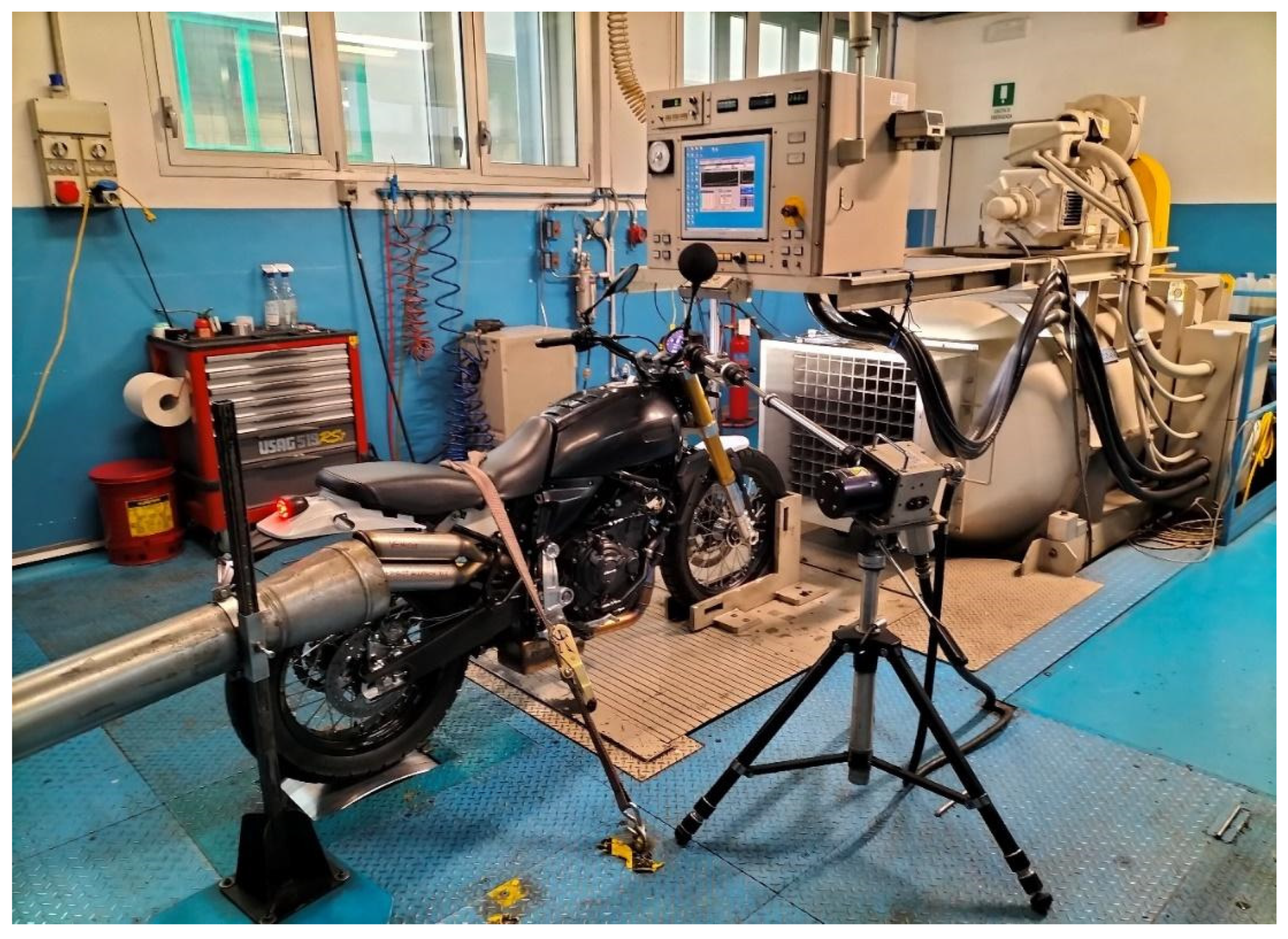
2. Materials and Methods

The main aim of this project is to use machine learning models to calibrate the injection volumetric efficiency of the engine targeting the lambda (air-to-fuel ratio), which is required by the ECU system. The air-to-fuel ratio primarily affects emissions, particularly when the engine is operating during the emission cycle loads. It also influences vehicle drivability and, crucially, performance—factors that are especially important for motorcycle engines. Regarding emissions, it is very important to maintain lambda within the stoichiometric zone (normally 1/1.5% in rich zone) in order to maintain catalyst efficiency. Drivability, especially for motorbikes, is very affected by torque variations due to air-to-fuel ratio oscillations; these variations are transmitted to the rear wheel, resulting in a harsh feeling when driving the motorcycle.
All the data used for this work were collected in the Motori Minarelli factory using an engine test cell equipped with a roller bench for testing the complete vehicle. The test bench—provided by Ono Sokki (Yokohama, Japan) [32]—is normally used for vehicle development; the motorcycle’s controls are fully automated except for gear shifting. For accurate estimation of air flow and replication of the motorcycle’s final behavior, it is essential that the vehicle is in the final production configuration, with all the components installed, such as the air filter, intake manifold, fairings, etc. As mentioned in the introduction, the tests were carried out with the whole vehicle because the focus of the work is on the final calibration process, with the intent of mass production.
The vehicle was braked by an eddy current dynamometer suitable for motorcycles, which develops up to 70 kW of peak power. The braking torques were set as a function of vehicle speed, following the coastdown curve, which was measured experimentally on a specific test road [33]. The test cell is equipped with traditional ventilation systems and additional systems to ensure a safe environment and compliance with test specifications. A large fan is positioned in front of the vehicle to simulate the variable air supply the motorcycle would experience when moving at a certain speed on the road; this feature is very important because air flows around the vehicle can affect air mass flow in the engine. Figure 1 shows the full experimental setup with the motorcycle at the test bench.
The setup that allows effective control over the vehicle during testing consists of a development ECU, which enables real-time monitoring and modification of engine parameters and calibration through analog/digital acquisition systems. Communication with the ECU is ensured by a Controller Area Network (CAN) connection to a PC, which uses the ETAS INCA (Stuttgart, Germany) [34] software for calibration, monitoring, diagnostics, and data acquisition. Other measurements, fuel consumption, engine torque, power, etc., were also acquired at the same time with a digital acquisition module by the test bench acquisition software.
In addition, an automatic system for motorcycle control manages the throttle, brake, and gearbox to achieve prescribed operational points and follow riding cycles efficiently. A test campaign was carried out driving the motorcycle with an automated cycle which can cover engine load from 1% to 100% at every engine speed (from 3000 RPM to 10,000 RPM) chosen for the acquisition. The test carried out for data acquisition consists of fixing the engine/vehicle speed (the gear does not change during the test) and varying the engine load from 1% to 100% in 60 s; this method allows the engine to reach a semi-transient condition. The data acquisition is performed continuously with a sampling frequency of 100 ms. The total duration of the test is 20 min.
The data were collected with a random calibration of the ECU in terms of volumetric efficiency of the engine. Random calibration was created starting from the production calibration with only one constraint: the value inserted is saturated at +−20%. The choice was made because of the measurement range of the UEGO sensor adopted (Bosch LSU 4.9).
In this work, different machine learning models were compared in terms of accuracy to find the best one for this particular application:
  • Gradient-Boosted Decision Tree Regressor [28]: This is a popular machine learning model consisting of an ensemble of decision trees trained sequentially. A decision tree is a non-parametric model that learns simple binary decision rules over the inputs—structured hierarchically in a tree—to approximate the target. The tree is constructed using the inputs and targets of the training data. To make a prediction for a test datapoint, the datapoint is “carried” along a branch of the tree according to how the inputs behave under the learned binary rules. Then, once a leaf is reached, the prediction is made using the average target values of the training datapoints that belong to that leaf. Decision trees are known to be prone to overfitting, and to be unable to learn very flexible decision boundaries: however, this can be significantly improved by “ensembling” multiple trees together. In particular, gradient-boosting is a technique whereby decision trees are sequentially fitted to the residual error (aka the “gradient”) of the previous tree.
  • Artificial Neural Network [35]: This class of models provides the highest level of flexibility in terms of the input-target relationships that can be learned. In particular, we focus on Feed-Forward Fully Connected Neural Networks. The fundamental building block of these is the perceptron, which takes as input a set of features, linearly combines them into a single value using learned weights and biases, and finally transforms said value with a simple nonlinear “activation” function. Multiple perceptrons can be combined in parallel, forming a layer, and layers are stacked, with the outputs of perceptrons in one layer being fed as inputs to the perceptrons in the next layer. Neural networks are trained using the backpropagation algorithm, whereby a loss function between the network’s output and the target is determined—in our case the Mean Squared Error loss—and the gradient of the loss value is backpropagated through the network using automatic differentiation; finally, the network parameters—weights and biases of the linear layers—are updated by taking a step in the direction of the gradient, using a predetermined learning rate.

3. Results

3.1. ECU Strategies and Calibrations

The main signals involved in estimating the engine combustion air flow are engine speed, usually expressed in Rotation Per Minute (RPM) and the Throttle Position Sensor (TPS) percentage. In some cases, the tests required either actively riding the motorcycle positioned on the roller, thus simulating normal road use, known as Auto Load Regulation (ALR), or using an electric actuator mechanically connected to the throttle control, adjusted via a potentiometer. This test setup, which can rotate the throttle grip from fully closed (0%) to fully open (100%) from outside the cell, is called Auto Speed Regulation (ASR). In this work, the data acquisition was performed by keeping vehicle speed constant, and by performing a sweeping of the load from 0 to 100% using ASP regulation.
Another parameter involved in estimating the engine combustion air flow is the Manifold Absolute Pressure (MAP), usually expressed in kPa and measured by a pressure sensor located in the motorcycle’s intake duct. This value mainly depends on the throttle opening and external atmospheric pressure. The ECU has a custom strategy for the estimation of the engine load. The load is considered in terms of TPS percentage if the TPS is greater than a threshold, which is a function of engine speed and TPS itself. If the threshold line is not crossed, the load is estimated by a MAP sensor. This strategy is mainly due to the sensitivity of TPS at low load; at this point, a small percentage of TPS opening corresponds to high gradients of air mass flow, thus leading to a worsening of the load estimation. Instead, the MAP sensor has a better resolution in small throttle opening, and thus is a more reliable parameter for estimating load.
Additionally, the motorcycle’s exhaust line is equipped with a linear lambda sensor (UEGO—Universal Exhaust Gas Oxygen sensor) capable of measuring the amount of oxygen in the exhaust gases, thereby providing the ECU with an estimate of the burnt mixture composition. This information allows the ECU to adjust the air-to-fuel ratio accordingly through automatic calibration with a Closed Loop (CL) algorithm. The CL strategy is active when the engine is running in stable condition, because in the case of high load gradient or high engine speed gradient the UEGO measurements lose accuracy. The adoption of a CL in this case could create instability in the air-to-fuel ratio. In these conditions, the ECU estimation is made only by calibrated models, and the amount of fuel injected is corrected only with environmental conditions (because these parameters are stable, and they do not enter into CL control).
UEGO signal and injection time are essential for calculating an indirect measure of the air flow into the engine. As mentioned above, the air mass flow is not directly measured with a specific sensor, due to calibration concerns. Indeed, introducing such a sensor would alter the intake line, affecting the mass flow it is trying to measure, thus not providing an accurate representation of what the mass flow would be without the sensor. The calculation of air mass flow is reported below in Equation (1):
m ˙ a i r = λ   α s t   t i n j   ρ F   G A I N i n j   1 10 6   60
where:
  • m ˙ a i r is the air flow rate expressed in mg c y c l e
  • λ is the lambda of the mixture
  • α s t is the stoichiometric air-fuel ratio, 14.65 in this case since the fuel is gasoline
  • t i n j is the injection time expressed in μ s
  • ρ F is the fuel density expressed in g dm 3 , in this case, it is 750 g dm 3
  • G A I N i n j is the injector gain, which is the quantity corresponding to the fuel flow rate deliverable by the model being used, expressed in cm 3 min , in this case, it is 280 cm 3 min
The response of the lambda sensor contains an intrinsic reading delay, which can be adjusted in various ways [36]. In this work, we take into consideration the time delay measurement presented by the universal exhaust gas oxygen sensor along with uncertainties in the volumetric efficiency. For that purpose, observers are designed by means of a super-twisting sliding mode estimation scheme. Also, two control schemes based on a general nonlinear model and a similar nonlinear affine representation for the dynamics of the normalized air to fuel ratio were designed in this work by using the super-twisting sliding mode methodology. Such dynamics depend on the control input, that is, the injected fuel mass flow, its time derivative, and its reciprocal. The two latter terms are estimated by means of a robust sliding mode differentiator. The observers and controllers are designed based on an isothermal mean value engine model. Numeric and hardware in-the-loop simulations were carried out with this model, the parameters being taken from a real engine. The results obtained show good output tracking and rejection of disturbances when the engine is in closed-loop with the proposed control. There are three main factors that influence this delay. The first is associated with the time interval between the opening of the intake valve and the exhaust valve, and is considered a combustion delay. The second factor represents the time it takes for the exhaust gases to reach the lambda sensor, depending on the air speed in the ducts, and is known as transmission delay. The third and final factor is related to the sensor itself, whose actual output is an aperiodic exponential curve, indicating a slow dynamic associated with a first-order system. The time constant can be approximately considered as 20 ms for a conventional sensor. The first two factors are clearly proportional to the engine’s rotational speed n , and can be expressed as follows [37]:
  • Combustion Delay:
T c = 3 4   120 n = 90 n
  • Transmission delay:
T e x h = 1 v e x h T c = 90 n

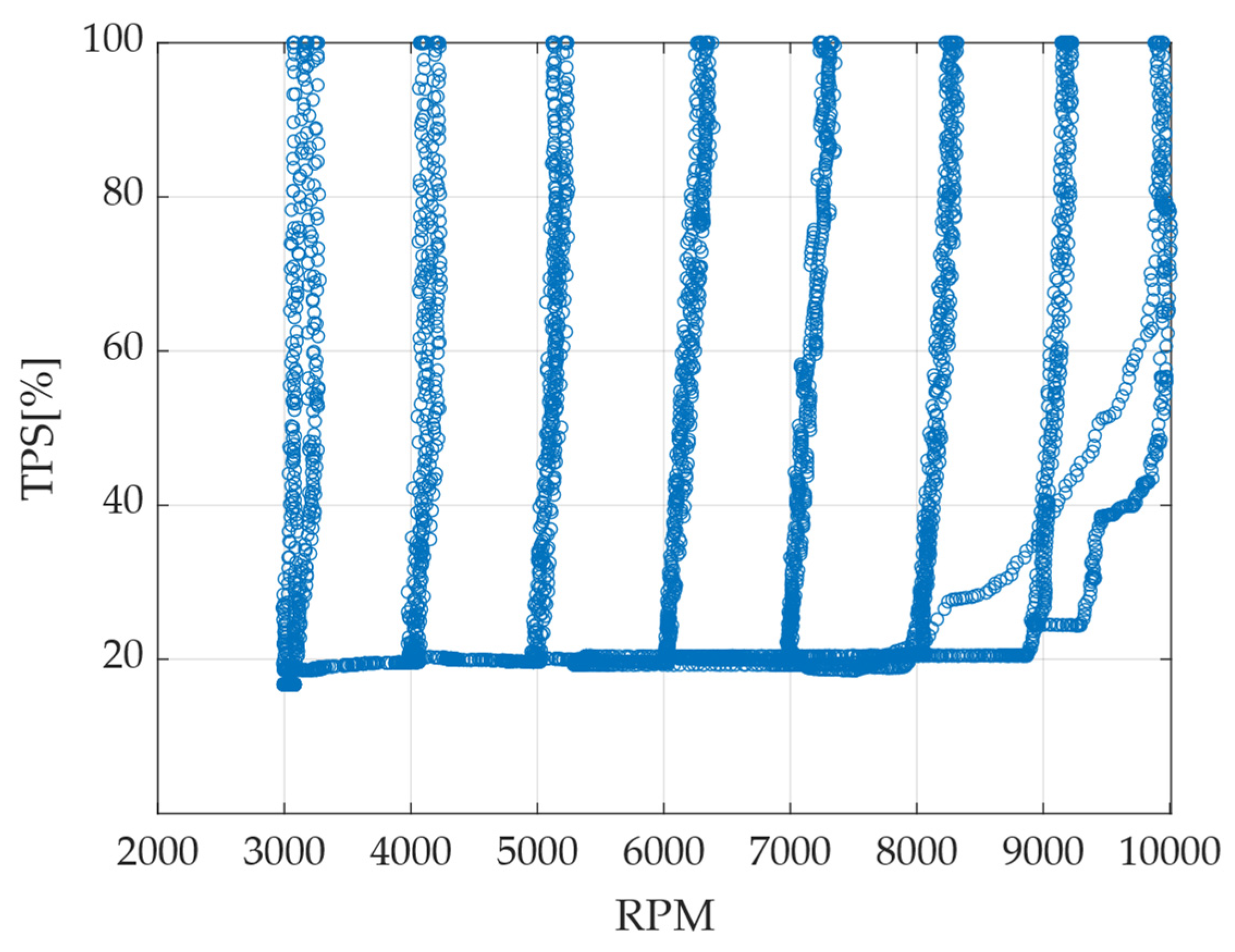
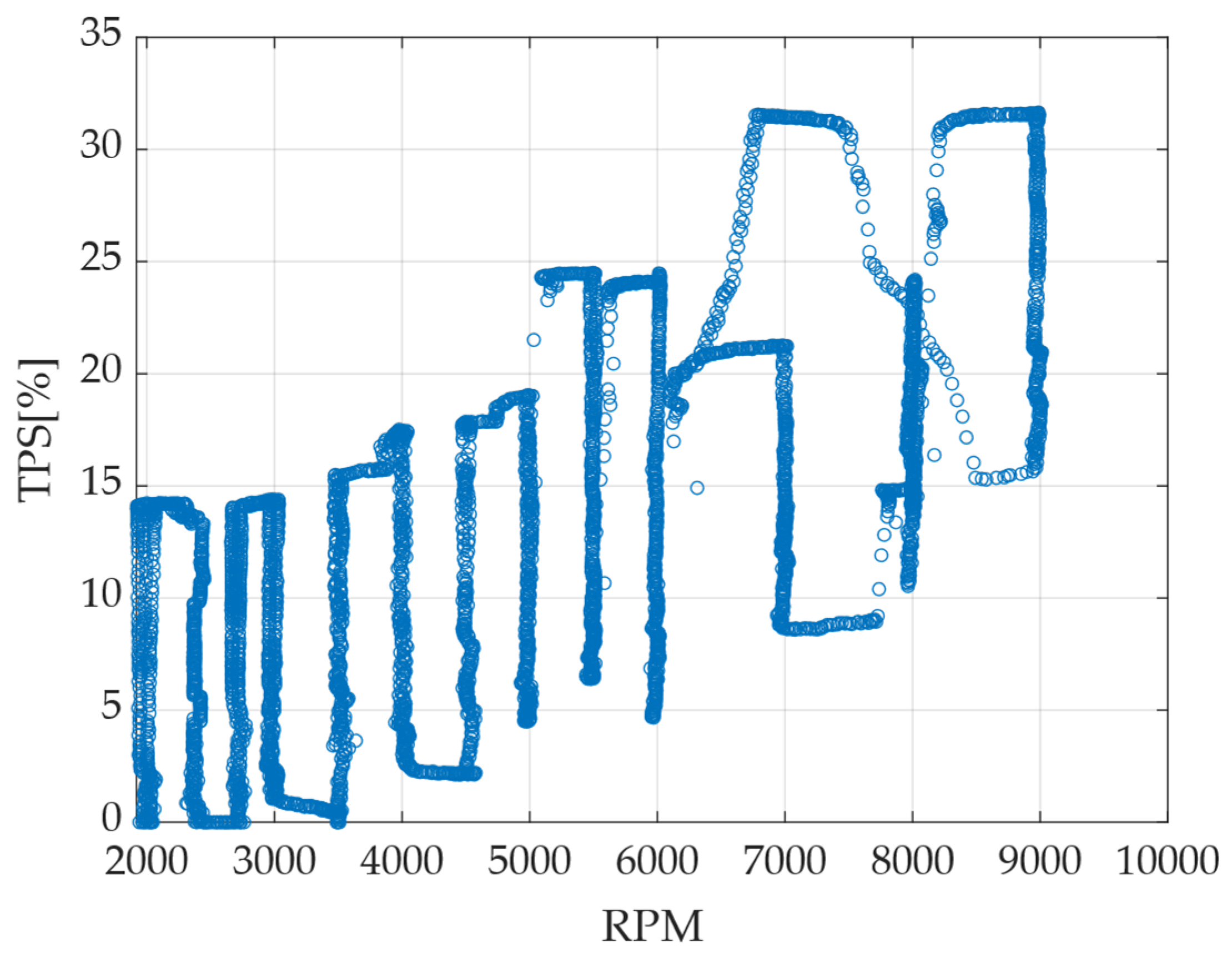
3.2. Data Training Acquisition and Creation of Models

The calibration, as already described, of injection timing in this engine is accomplished using two different strategies. The first is called Speed Density (SD) and is based on engine speed (RPM) and MAP. This strategy is primarily used at low loads where the estimation derived only from the throttle position is insufficient. The second strategy is called Alpha Speed (AS), it is expressed in terms of engine speed (RPM) and TPS, and it covers the remaining operating range of the engine. The two strategies are separated by an RPM-TPS threshold vector, which determines which strategy has to be used for determining the injection timing [38,39]. For training the machine learning models, two different data acquisition processes were performed, one for each strategy. Figure 2 and Figure 3 show the investigated operating points for the SD and AS strategies, respectively. The data acquisition was designed to cover all boundaries of the engine in terms of load and speed. The data acquisition system sampling frequency is set to 100 ms. For each strategy (AS, SD), the engine speed is held fixed at different values, and the load is swept from 0% to 100% within each strategy’s boundaries, thus resulting in a “striped” acquisition pattern. The total time of data acquisition is approximately 20 min, and each parameter is sampled at 100 ms [8]. The maneuvers performed can be considered almost in steady-state condition. The approach adopted is well-suited to the experimental setup (roller bench) and offers significant time savings in data acquisition without compromising accuracy, thanks to the slow transition between measurement points. This method contrasts with traditional data acquisition for machine learning models, which is usually performed under steady-state conditions on the engine test bench. The Design of Experiment (DOE) has been chosen for time vs accuracy in case a whole vehicle is used for the data collecting. A full factorial approach is not useful since every point would need acceleration and braking of the vehicle, and the time to reach the steady state would increase for every point reached. It is crucial to clearly define the boundaries of the problem being studied to avoid extrapolations that could reduce the accuracy of the regression model estimates. The data acquired were filtered before being used by the algorithms to isolate only the points contained in each strategy. The two datasets were used to discriminate the adoption of the TPS sensor or MAP sensor signal as input for the ML model.
The training datasets are derived from data acquisition, applying some post-processing constraints and calculations. First, the measurement errors were filtered out, and secondly, the UEGO signal was delayed as described in the previous section. The data was divided between AS and SD, and the model was created with different load input signals (TPS or MAP). Figure 4 shows the range within which machine learning models can be used successfully. On the left, a brief acquisition related to the Speed Density strategy is shown, where only a few load sweeps at constant RPM can be observed. This dataset is used to train the predictive model. On the right, a dataset produced in MATLAB R2023b is shown which, with a certain level of discretization, queries the machine learning algorithm at all the engine operating points that fall within the injection strategy (in this case SD).
The machine learning model was created using the throttle position sensor, the MAP sensor, and the engine rotational speed as inputs. The generated output is the airflow rate. Models with additional inputs (ambient pressure, ambient temperature, engaged gear, throttle opening derivative) were tested and developed, but they resulted in poorer performance. This outcome is due to the fact that the combustion engine under analysis does not have variable valve timing systems, and the airflow rate is solely linked to those parameters. Furthermore, the pressure and temperature conditions in the test cell are constant, as there is a conditioning system in the test room. Models were created using the functions “fitrnet” and “fitrensemble” included in MATLAB Toolbox “Statistics and Machine Learning”. The first was used for feed-forward fully-connected neural networks, and the second for tree ensembles. We used Bayesian Optimization—natively integrated in both functions—to find the best configurations of hyperparameters. This algorithm is iterative and able to search through various possibilities to minimize the objective function, which in this case is the expression log(1+loss), where the loss is the mean square error (MSE) that is calculated with the current iteration hyperparameter configuration. In this work, multiple iterations of optimization are used to ensure that the results were comparable and repeatable across different runs of the code, and this was indeed the case. In fact, the Bayesian algorithm implemented in MATLAB almost always provides a different combination of hyperparameters compared to the previous result, but the performance that the models achieve is very similar. For this reason, the described models can be considered representative of their respective categories.
For the Alpha Speed injection strategy, several experimental trials have identified the neural network as the best model. The one in consideration is composed by two hidden layers (the first with 155 neurons and the second with 239), ReLU activation function, Glorot initialization of weights, and LBFGS as training solver algorithm. For Speed Density, a tree ensemble with Least Squares Boost algorithm (gradient boosted trees), 49 sequential decision trees, a learning rate of approximately 0.21, one as the minimum number of observations per leaf node, 69 as the maximum number of decision splits, and two as the number of features to randomly select for each split, seems to be the best choice in terms of model performance (Table 1).
Figure 5 shows on the x axis the measured air mass flow, and on the y axis the estimated air mass flow; for the sake of brevity, only the predictions of the gradient boosted tree model are shown here. The model was created by excluding outlier points. It can be observed that there is good agreement between the model predictions and real air mass flow.

4. Discussion

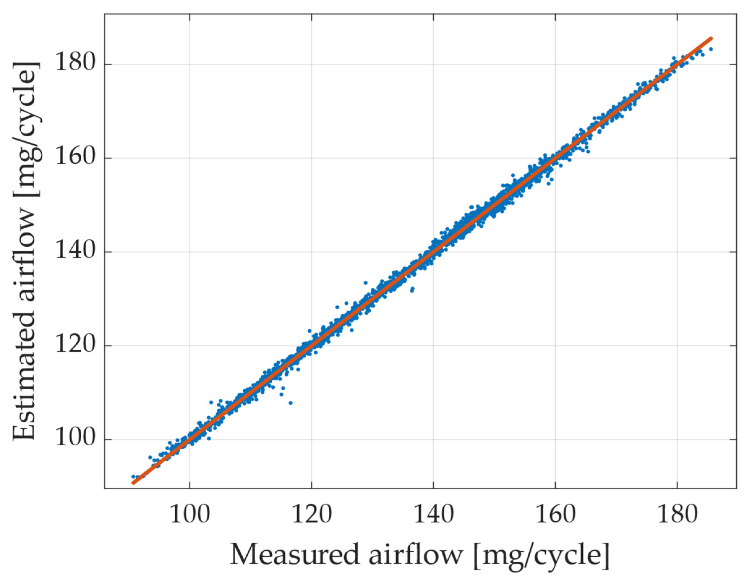
4.1. Model Perfomance Evalutation

Once the machine learning models produce acceptable performance in predicting the air flow rate, the estimated injection times are derived using Equation (1) and the target lambda, and are then inputted into the ECU. With these, the complete map can be compiled and uploaded to the ECU. If, as in the case at hand, injection times obtained from the bench using the standard experimental method are available and thus serve as the target values for the models to achieve, comparison errors can be calculated. These errors can guide potential improvements in the structure and the choice of hyperparameters for the machine learning models.
e r r p e r c = t i n j t a r g e t t i n j m o d e l 100 100
In this way, the following results were obtained, clearly highlighting where the models used produce injection times that deviate most from the targets. Regarding the Alpha Speed strategy, a neural network was used with results shown in Figure 6.
It can be seen that only certain engine speeds were measured, but even for the unstudied speeds, as long as they are interpolated between speeds in the training data, the estimated injection times produce very low errors. Speeds at the borders of the training range instead show higher errors; this result was expected because machine learning models struggle at extrapolation. The highest error values occur just below the maximum engine RPM, at throttle openings of 90% and above. This is because, in that range, being close to the limit, very few data were acquired on the test bench. At 10,000 RPM, no samples were measured. The average absolute percentage error is 2.5%, while the standard deviation is 2.8.
In Figure 7, we try to understand whether a relationship exists between percentage error and injection time. The goal is to exclude the possibility that low errors are due to a link with high injection times and vice versa. This could distract the user from the actual evaluation of the model. As can be seen, the two variables appear to be uncorrelated, as the scatter plot, despite its dispersion, does not exhibit any particular trend with increasing injection time.
Figure 8 and Figure 9 show analogous results for the Speed Density strategy, using a gradient boosted decision tree model.

4.2. Motorcycle Calibration Validation

Finally, the calibrated map, calculated from the models starting from the air-to-fuel ratio required by the ECU calibration, was flashed into the vehicle. The vehicle was tested at the test bench in Road Load Control (RLC) with a real driver, to evaluate the performance of the calibration created by ML models. During these acquisitions, the usual engine parameters were measured, including MAP, various temperatures and pressures, and the lambda value measured by the sensor, as well as the target lambda channel, which is automatically calculated by the control unit through interpolation based on RPM and TPS relative to the point of interest. At Motori Minarelli, as in many other companies in the sector, calibrators use two thresholds around the target lambda value to describe an acceptable range for the measured lambda signal produced by combustion. In this case, the acceptable numbers must fall within +/−3.5% of the target during engine operation [16].
The results at high engine loads are reported in Figure 10 (AN strategy), whereas results at low loads are shown in Figure 11 (SD strategy). In terms of the latter, it was necessary to redo the training data acquisition for the machine learning models, repeating the maneuvers more slowly and achieving a finer discretization of points than the first attempt. In fact, at low loads and low engine speeds, small variations in TPS percentage correspond to large changes in the MAP signal (tens of KPa in pressure).
The maneuvers were performed without high load gradient, because the fluid compensation film, which corrects the fuel mass flow, was not modeled and thus not evaluated. Each figure consists of two graphs. The upper graph shows the derivate of TPS [%/s] to evaluate if the maneuver was performed with slow gradient; the lower graph shows the lambda target required by the system (in red), the lambda signal measured (in blue), and an offset of the target of +−3.5% (dotted black) which represents the limit for an acceptable calibration. It can be seen that the lambda measurement coincides with the dotted lines; this evidence shows the good accuracy of the estimation. Only part of the dataset shows a lambda signal outside of the acceptable limits, but these points are not of interest because they are related to gear shifting or engine speed limiter interventions, which affect lambda signal because of cutoff or misfire, which can occur in these conditions.
Using the proposed approach, the reduction in calibration time, when compared to a conventional calibration process which requires approximately four days to complete, has been estimated at around 80%. It is important also to note that, in vehicle development, this calibration process is repeated multiple times, one for each modification made during the design phase (e.g., update of intake manifold, frame, fairings, driver seat, fuel tank, wiring, exhaust system). As a result, the benefits of employing machine learning models are compounded, ultimately leading to significant savings in both time and costs.

4.3. DOE Evaluation

A brief Design of Experiment (DOE) was then conducted to study how the performance of the models changed as a function of the number of points acquired for the training datasets (Figure 12). The objective was to obtain a grid that can be used in any acquisition context, which determines a minimum standard number of samples. This goal was achieved by attempting to discretize as uniformly as possible, especially at the boundaries, to avoid model extrapolation. A substantial portion of points was therefore eliminated, up to approximately 95% of the samples, i.e., from 4800 observations to about 70 operating points. The results obtained show the potential margin for improvement in the selection of key samples for model training [40].
The main reason for this result is related to the type of experimental setup. When using an entire vehicle on the roller bench, many acquisition points are essentially overlapping. However, it is interesting to note that acquisition can be performed more quickly and with the help of acquisition systems that also operate at low frequencies. The decision to use the entire vehicle was made because the goal of calibrating the complete system requires using the vehicle with all its parts. Conversely, for a less advanced engine development phase, the engine test bench would be more appropriate to optimize the DOE structure and measurement times.
This work has enabled a reduction in the engine air flow calibration procedures by about one-fifth compared to the traditional procedure, without losing points of accuracy. The errors recorded during the modeling campaign are, in fact, comparable to the uncertainties of the measurement chain.

5. Conclusions

The main aim of this work is to demonstrate the potential of machine learning models for calibrating a complete motorcycle setup, chosen for its high accuracy requirements in production vehicles. Focusing on motorcycles, air-to-fuel ratio calibration is crucial not only for emissions and consumption but also for the instantaneous torque of the engine; therefore, small oscillations in lambda can significantly affect vehicle drivability.
The presented results show a completely new methodological approach, from the experimental setup to the model validation, and its direct application to the production vehicle. It has been demonstrated that this methodology can drastically reduce the calibration effort needed to fine-tune the vehicle at the production stage, without reducing accuracy. The machine learning models employed, particularly regression and neural network algorithms, have demonstrated their capability to accurately predict the optimal calibration parameters based on limited experimental data.
These models can prove advantageous not only in test bench conditions but also in a whole vehicle, demonstrating significant potential for other calibration.
The reduction in calibration time compared to a conventional calibration process has been estimated at around 80%, as traditional calibration takes approximately four days to complete.

Author Contributions

Conceptualization T.S., C.A.R., M.P., L.E. and G.V.; Data curation T.S., M.P., L.E. and G.V.; Writing T.S., C.A.R., M.P., L.E. and G.V.; Validation C.A.R., M.P., L.E. and G.V. All authors have read and agreed to the published version of the manuscript.

Funding

This research received no external funding.

Data Availability Statement

The data presented in this study are available on request from the corresponding author.

Acknowledgments

All authors would like to acknowledge Motori Minarelli for the support offered during the experimental process of this project.

Conflicts of Interest

Authors T. Savioli and M. Pampanini were employed by the company Atris Engineering srl. Author L. Esposito was employed by the company Motori Minarelli spa. The remaining authors declare that the research was conducted in the absence of any commercial or financial relationships that could be construed as a potential conflict of interest.

Abbreviations

ANNArtificial Neural Network
ECUEngine Control Unit
CANControlled Area Network
TPSThrottle Position Sensor
ALRAuto Load Regulation
ASRAuto Speed Regulation
UEGOUniversal Exhaust Gas Oxygen sensor
MAPManifold Absolute Pressure
CLClosed Loop
SDSpeed Density
ASAlfa Speed
DOEDesign Of Experiment
RLCRoad Load Control

References

  1. Martyr, A.J.; Plint, M.A. Engine Testing: Theory and Practice; Elsevier: Amsterdam, The Netherlands, 2011; ISBN 978-0-08-052472-6. [Google Scholar]
  2. Johnson, T.; Joshi, A. Review of Vehicle Engine Efficiency and Emissions. SAE Int. J. Engines 2018, 11, 1307–1330. [Google Scholar] [CrossRef]
  3. Ashok, B.; Ashok, S.D.; Kumar, C.R. A review on control system architecture of a SI engine management system. Annu. Rev. Control. 2016, 41, 94–118. [Google Scholar] [CrossRef]
  4. Castagné, M.; Bentolila, Y.; Chaudoye, F.; Hallé, A.; Nicolas, F.; Sinoquet, D. Comparison of Engine Calibration Methods Based on Design of Experiments (DoE). Oil Gas Sci. Technol. Rev. d’IFP Energies Nouv. 2008, 63, 563–582. [Google Scholar] [CrossRef]
  5. Suykens, J.A.; Vandewalle, J.P.; De Moor, B.L. Artificial Neural Networks for Modelling and Control of Non-Linear Systems; Springer International Publishing: Cham, Switzerland, 2012; ISBN 978-1-4757-2493-6. [Google Scholar]
  6. Samadani, E.; Shamekhi, A.H.; Behrouzi, M.; Chini, R. A method for pre-calibration of DI diesel engine emissions and performance using neural network and multi-objective genetic algorithm. SID 2009, 28, 61–70. [Google Scholar]
  7. Turkson, R.F.; Yan, F.; Ali, M.K.A.; Hu, J. Artificial neural network applications in the calibration of spark-ignition engines: An overview. Eng. Sci. Technol. Int. J. 2016, 19, 1346–1359. [Google Scholar] [CrossRef]
  8. De Simio, L.; Iannaccone, S.; Iazzetta, A.; Auriemma, M. Artificial neural networks for speeding-up the experimental calibration of propulsion systems. Fuel 2023, 345, 128194. [Google Scholar] [CrossRef]
  9. Boccardo, G.; Piano, A.; Zanelli, A.; Babbi, M.; Cambriglia, L.; Mosca, S.; Millo, F. Development of a virtual methodology based on physical and data-driven models to optimize engine calibration. Transp. Eng. 2022, 10, 100143. [Google Scholar] [CrossRef]
  10. Yang, R.; Yan, Y.; Sun, X.; Wang, Q.; Zhang, Y.; Fu, J.; Liu, Z. An Artificial Neural Network Model to Predict Efficiency and Emissions of a Gasoline Engine. Processes 2022, 10, 204. [Google Scholar] [CrossRef]
  11. Jaliliantabar, F.; Ghobadian, B.; Najafi, G.; Yusaf, T. Artificial Neural Network Modeling and Sensitivity Analysis of Performance and Emissions in a Compression Ignition Engine Using Biodiesel Fuel. Energies 2018, 11, 2410. [Google Scholar] [CrossRef]
  12. Ziółkowski, J.; Oszczypała, M.; Małachowski, J.; Szkutnik-Rogoż, J. Use of Artificial Neural Networks to Predict Fuel Consumption on the Basis of Technical Parameters of Vehicles. Energies 2021, 14, 2639. [Google Scholar] [CrossRef]
  13. Brahma, I.; Sharp, M.C.; Richter, I.B.; Frazier, T.R. Development of the nearest neighbour multivariate localized regression modelling technique for steady state engine calibration and comparison with neural networks and global regression. Int. J. Engine Res. 2008, 9, 297–323. [Google Scholar] [CrossRef]
  14. Meli, M.; Wang, Z.; Bailly, P.; Pischinger, S. Neural Network Modeling of Black Box Controls for Internal Combustion Engine Calibration; SAE Technical Paper 2024-01–2995; SAE International: Warrendale, PA, USA, 2024. [Google Scholar] [CrossRef]
  15. de Nola, F.; Giardiello, G.; Gimelli, A.; Molteni, A.; Muccillo, M.; Picariello, R. Volumetric efficiency estimation based on neural networks to reduce the experimental effort in engine base calibration. Fuel 2019, 244, 31–39. [Google Scholar] [CrossRef]
  16. Zhou, H.; Li, X.; Lee, C.-F.F. Investigation on soot emissions from diesel-CNG dual-fuel. Int. J. Hydrogen Energy 2019, 44, 9438–9449. [Google Scholar] [CrossRef]
  17. Pan, T.; Cai, Y.; Chen, S. Development of an Engine Calibration Model Using Gaussian Process Regression. Int. J. Automot. Technol. 2021, 22, 327–334. [Google Scholar] [CrossRef]
  18. Jacob, A.; Ashok, B. An interdisciplinary review on calibration strategies of engine management system for diverse alternative fuels in IC engine applications. Fuel 2020, 278, 118236. [Google Scholar] [CrossRef]
  19. Rahimi-Gorji, M.; Ghajar, M.; Kakaee, A.-H.; Ganji, D.D. Modeling of the air conditions effects on the power and fuel consumption of the SI engine using neural networks and regression. J. Braz. Soc. Mech. Sci. Eng. 2017, 39, 375–384. [Google Scholar] [CrossRef]
  20. Garg, A.B.; Diwan, P.; Saxena, M. Artificial neural networks based methodologies for optimization of engine operations. Int. J. Sci. Eng. Res. 2012, 3, 1–5. [Google Scholar]
  21. Shayler, P.; Goodman, M.; Ma, T. The exploitation of neural networks in automotive engine management systems. Eng. Appl. Artif. Intell. 2000, 13, 147–157. [Google Scholar] [CrossRef]
  22. Schoeggl, P.; Ramschak, E. Vehicle Driveability Assessment Using Neural Networks for Development, Calibration and Quality Tests; SAE Technical Paper 2000-01–0702; SAE International: Warrendale, PA, USA, 2000. [Google Scholar] [CrossRef]
  23. Atkinson, C.; Mott, G. Dynamic Model-Based Calibration Optimization: An Introduction and Application to Diesel Engines; SAE Technical Paper 2005-01–0026; SAE International: Warrendale, PA, USA, 2005. [Google Scholar] [CrossRef]
  24. Lowe, D.; Zapart, C. Point-Wise Confidence Interval Estimation by Neural Networks: A Comparative Study based on Automotive Engine Calibration. Neural Comput. Appl. 1999, 8, 77–85. [Google Scholar] [CrossRef]
  25. Friedrich, C.; Auer, M.; Stiesch, G. Model Based Calibration Techniques for Medium Speed Engine Optimization: In-vestigations on Common Modeling Approaches for Modeling of Selected Steady State Engine Outputs. SAE Int. J. Engines 2016, 9, 1989–1998. [Google Scholar] [CrossRef]
  26. Vinoth, B.; Uma, G.; Umapathy, M. Recurrent Neural Network based Soft Sensor for flow estimation in Liquid Rocket Engine Injector calibration. Flow Meas. Instrum. 2022, 83, 102105. [Google Scholar] [CrossRef]
  27. Breiman, L. Random forests. Mach. Learn. 2001, 45, 5–32. [Google Scholar] [CrossRef]
  28. Friedman, J.H. Greedy function approximation: A gradient boosting machine. Ann. Stat. 2001, 29, 1189–1232. [Google Scholar] [CrossRef]
  29. Grinsztajn, L.; Oyallon, E.; Varoquaux, G. Why do tree-based models still outperform deep learning on typical tabular data? Adv. Neural Inf. Process. Syst. 2022, 35, 507–520. [Google Scholar]
  30. Liu, J.; Ulishney, C.; Dumitrescu, C.E. Random Forest Machine Learning Model for Predicting Combustion Feedback Information of a Natural Gas Spark Ignition Engine. J. Energy Resour. Technol. 2020, 143, 012301. [Google Scholar] [CrossRef]
  31. Kefalas, A.; Ofner, A.B.; Pirker, G.; Posch, S.; Geiger, B.C.; Wimmer, A. Estimation of Combustion Parameters from Engine Vibrations Based on Discrete Wavelet Transform and Gradient Boosting. Sensors 2022, 22, 4235. [Google Scholar] [CrossRef]
  32. Ono Sokki Official Website. Available online: https://www.onosokki.net/ (accessed on 7 October 2024).
  33. Preda, I.; Covaciu, D.; Ciolan, G. Coast Down Test—Theoretical and Experimental Approach; Transilvania University Press: Brașov, Romania, 2010. [Google Scholar]
  34. INCA Base Product. ETAS Group. Available online: https://www.etas.com (accessed on 7 October 2024).
  35. Jain, A.; Mao, J.; Mohiuddin, K. Artificial neural networks: A tutorial. Computer 1996, 29, 31–44. [Google Scholar] [CrossRef]
  36. Espinoza-Jurado, J.; Dávila, E.; Rivera, J.; Raygoza-Panduro, J.J.; Ortega, S. Robust Control of the Air to Fuel Ratio in Spark Ignition Engines with Delayed Measurements from a UEGO Sensor. Math. Probl. Eng. 2015, 2015, 989674. [Google Scholar] [CrossRef]
  37. Meng, L.; Wang, X.; Zeng, C.; Luo, J. Adaptive Air-Fuel Ratio Regulation for Port-Injected Spark-Ignited Engines Based on a Generalized Predictive Control Method. Energies 2019, 12, 173. [Google Scholar] [CrossRef]
  38. Zhai, Y.-J.; Yu, D.-L. A Neural Network Model Based MPC of Engine AFR with Single-Dimensional Optimization. In Advances in Neural Networks—ISNN 2007; Liu, D., Fei, S., Hou, Z.-G., Zhang, H., Sun, C., Eds.; Springer: Berlin/Heidelberg, Germany, 2007; pp. 339–348. ISBN 978-3-540-72383-7. [Google Scholar] [CrossRef]
  39. Uzun, A. Air mass flow estimation of diesel engines using neural network. Fuel 2014, 117, 833–838. [Google Scholar] [CrossRef]
  40. Pontes, F.J.; Amorim, G.F.; Balestrassi, P.P.; Paiva, A.P.; Ferreira, J.R. Design of experiments and focused grid search for neural network parameter optimization. Neurocomputing 2016, 186, 22–34. [Google Scholar] [CrossRef]
Figure 1. Whole test bench setup.
Fluids 09 00239 g001
Figure 2. Measured operation points (high load).
Fluids 09 00239 g002
Figure 3. Measured operation points (low load).
Fluids 09 00239 g003
Figure 4. Training dataset vs. testing dataset.
Fluids 09 00239 g004
Figure 5. Measured vs. predicted airflow with gradient boosted trees.
Fluids 09 00239 g005
Figure 6. Percentage error in comparison to original calibration map (Alpha Speed). The cells highlighted in red represent model-estimated injection times that are lower than the target values, while the green cells indicate injection times that are higher than the target.
Fluids 09 00239 g006
Figure 7. Percentage error vs. injection timing (Alpha Speed).
Fluids 09 00239 g007
Figure 8. Percentage error in comparison to original calibration map (Speed Density). The cells highlighted in red represent model-estimated injection times that are lower than the target values, while the green cells indicate injection times that are higher than the target.
Fluids 09 00239 g008
Figure 9. Percentage error vs. injection timing (Speed Density).
Fluids 09 00239 g009
Figure 10. Vehicle data acquisition for Alpha Speed with ECU map created by IA.
Fluids 09 00239 g010
Figure 11. Vehicle data acquisition for Speed Density with ECU map created by IA.
Fluids 09 00239 g011
Figure 12. Mean percentage error vs. operating points.
Fluids 09 00239 g012
Table 1. Model setup.
Injection StrategyAlpha SpeedSpeed Density
Model typeNeural networkGradient boosted trees
Model features
  • Bayesian optimization
  • Feed-forward fully connected
  • [115,239] neurons
  • ReLU activation function
  • Glorot weights initialization
  • LBFGS training solver algorithm
  • Bayesian optimization
  • LS Boost algorithm
  • 49 sequential trees
  • Learning rate of 0.21
  • 1 minimum observation per leaf
  • 69 maximum decision splits
  • 2 features per split
Disclaimer/Publisher’s Note: The statements, opinions and data contained in all publications are solely those of the individual author(s) and contributor(s) and not of MDPI and/or the editor(s). MDPI and/or the editor(s) disclaim responsibility for any injury to people or property resulting from any ideas, methods, instructions or products referred to in the content.

