Computation of Real-Fluid Thermophysical Properties Using a Neural Network Approach Implemented in OpenFOAM

Abstract

Machine learning based on neural networks facilitates data-driven techniques for handling large amounts of data, either obtained through experiments or simulations at multiple spatio-temporal scales, thereby finding the hidden patterns underlying these data and promoting efficient research methods. The main purpose of this paper is to extend the capabilities of a new solver called realFluidReactingNNFoam, under development at the University of Perugia, in OpenFOAM with a neural network algorithm for replacing complex real-fluid thermophysical property evaluations, using the approach of coupling OpenFOAM and Python-trained neural network models. Currently, neural network models are trained against data generated using the Peng–Robinson equation of state assuming a mixture’s frozen temperature. The OpenFOAM solver, where needed, calls the neural network models in each grid cell with appropriate inputs, and the returned results are used and stored in suitable OpenFOAM data structures. Such inference for thermophysical properties is achieved via the “Neural Network Inference in C made Easy (NNICE)” library, which proved to be very efficient and robust. The overall model is validated considering a liquid-rocket benchmark comprised of liquid-oxygen (LOX) and gaseous-hydrogen (GH2) streams. The model accounts for real-fluid thermodynamics and transport properties, making use of the Peng–Robinson equation of state and the Chung transport model. First, the development of a real-fluid model with an artificial neural network is described in detail. Then, the numerical results of the transcritical mixing layer (LOX/GH2) benchmark are presented and analyzed in terms of accuracy and computational efficiency. The results of the overall implementation indicate that the combined OpenFOAM and machine learning approach provides a speed-up factor higher than seven, while preserving the original solver accuracy.

1. Introduction

This introduction provides an overview of the historical and evolving role of machine learning (ML) in computational fluid dynamics (CFD), highlighting its transformative potential across numerous applications. As we delve deeper into the intersection of ML and CFD, we will explore specific methodologies, case studies, and emerging trends that underscore the symbiotic relationship between these two fields, ultimately reshaping our understanding of fluid dynamics and propelling innovation in diverse industries.

Admittedly, much progress has been made in recent years to promote our understanding of combustion from a computational perspective, for example by analyzing hydrogen high-pressure injection and mixing processes [1], including the assessment of a model which accounts for real-fluid thermodynamics and transport properties, making use of the Peng–Robinson equation of state (PR-EoS) and the Chung transport model [2]. Reitz and co-workers focused on a thermodynamic analysis of mixture states [3]. The challenges primarily come from real-gas effects, which have significant effects on these processes, introducing nonlinearities into thermodynamic systems resulting in non-physical pressure oscillations that can substantially affect accuracy. Accurate data in states near critical point are also difficult to obtain from both experiments and models.

Numerous theoretical and experimental studies, such as Puissant et al.’s investigations on shear coaxial injection [4] and Mayer’s understanding of LOX/GH2 rocket engine combustion processes [5], have been conducted on high-pressure flows. These studies aim to gain insight into chemical and physical processes, providing a database for improved modeling and the validation of simulation codes for combustor design and optimization [6]. Analyzing hydrogen high-pressure injection in the near-nozzle region, investigating the formation process and the structure of the Mach disks and the transition to turbulent jets, has been undertaken by Rahantamialisoa et al. [7], and Oschwald et al. [8] present experiments on inert binary injection and mixing processes.

To accurately model these behaviors with thermodynamic non-idealities and transport anomalies [9], a generalized EoS valid for the entire thermodynamic fluid regime is necessary. However, employing such a highly nonlinear EoS, especially in problems involving multiple species and multiscale physics, is computationally expensive. For instance, in large eddy simulations (LESs) of supercritical reacting jets or mixing layers, significant computational time is dedicated to evaluating real-fluid properties using EoSs like PR or Soave–Redlich–Kwong (SRK) [10,11,12,13].

In response to these challenges, a deep-learning based approach, termed deep feedforward neural network (NN) with boundary conditions, has been developed for the efficient evaluation of thermophysical properties in complex real-fluid flows [14]. This approach replaces the direct calculation of the EoS with a NN trained with appropriate boundary information, significantly improving computational efficiency. Furthermore, addressing the fundamental Riemann problem in CFD codes for simulating compressible flows, fully connected feedforward NNs have been employed to find solutions for real fluids, including calorically imperfect gases, supercritical fluids, and high explosives [15]. These NNs, embedded into a one-dimensional finite volume CFD code, yield remarkable speed-ups of up to five orders of magnitude compared to exact solvers, with prediction errors below 0.8%.

Using tabulation, ML and artificial NN models for tackling the complex issue of transcritical sprays, which are relevant to modern compression-ignition engines, can assist the speeding up of calculations. Direct simulations can incur significant CPU costs, whereas tabulation may be memory-intensive and challenging to expand as the number of chemical species grows [16,17]. In contrast, NNs have emerged as a remarkably efficient technique for classification and response prediction. In high-pressure, high-temperature conditions, NN methods are used to predict thermodynamic properties [18], and the tabulation method offers high-precision calculation results in a wide temperature and pressure range [16,17]. ML techniques are rapidly advancing in this era of big data, and there is high potential in exploring the combination between ML and combustion research and achieving remarkable results. Much of this interest is attributed to the remarkable performance of deep learning architectures, which hierarchically extract informative features from data [19]. R. Maulik et al. demonstrate the deployment of a deep neural network for compressing flow-field information using an autoencoder to demonstrate the ability to use state-of-the-art ML tools in the Python ecosystem [20,21]. In the realm of fluid mechanics, NNs are currently being explored as a complementary tool of CFD to expedite design processes [18]. Recent comprehensive reviews have highlighted various applications in fluid mechanics, encompassing flow feature extraction, turbulence modeling, optimization, and flow control [19]. Also in the energy sector, iterative-learning approaches are used to enhance model reliability by iteratively updating supervised training datasets to refine correlations, or by adopting deep learning-based prediction methods [22,23]. In the near future, the necessity will arise for designing adaptable energy production and propulsion systems that can efficiently utilize a wide range of fuels, including synthetic, bio-derived, and fossil fuels, or various combinations thereof. Modeling these fuels, especially when their properties are not initially known, will demand flexible methods that can describe essential operational traits with minimal input data.

Present Contribution

To achieve the above objectives, extending the work by Koukouvinis et al. [18], we propose the application of ML to provide quantitative CFD predictions involving real-fluid mixtures under unknown conditions, with reduced computational costs and comparable accuracy.

Specifically, this work discusses the capabilities of a new solver called realFluidReactingNNFoam, using a NN algorithm for replacing complex real-fluid thermophysical property evaluations using the approach of coupling OpenFOAM-v2112 and Python-developed models.

2. Mathematical Models and Implementations

2.1. CFD Model

The governing equations for a fully conservative, homogeneous, multicomponent, and compressible non-reacting two-phase flow are the conservation equations for mass, momentum, energy, and species, which are written below [2,21,24,25]:

$$\frac{\partial \rho }{\partial t}+\nabla ·\left(\rho \mathbf{U}\right)=0$$

(1)

$$\frac{\partial \left(\rho \mathbf{U}\right)}{\partial t}+\nabla ·\left(\rho \mathbf{U}\mathbf{U}\right)=\nabla ·\left(-p\mathbf{I}+\mathit{\tau }\right)$$

(2)

$$\frac{\partial \left(\rho h_T\right)}{\partial t}+\nabla ·\left(\rho h_T\mathbf{U}\right)=\frac{\partial p}{\partial t}+\nabla ·\left(\mathbf{U}·\mathit{\tau }\right)-\nabla ·\mathbf{q}$$

(3)

$$\frac{\partial \left(\rho Y_k\right)}{\partial t}+\nabla ·\left(\rho Y_k\mathbf{U}\right)=-\nabla ·{\mathbf{J}}_k$$

(4)

In the above equations, $\rho$ is the mixture density, $\mathbf{U}$ is the mixture velocity vector, $p$ is the pressure shared by all species, $\mathit{\tau }$ is the viscous stress tensor of the mixture, $Y_k$ is the mass fraction of species k, and ${\mathbf{J}}_k$ and $\mathbf{q}$ refer to diffusion flux of species $k$ and heat flux, respectively. Also, $h_T=h+1/2{\mathrm{U}}^2$ is the total enthalpy of the mixture.

Additionally, for the evaluation of thermodynamic fluid properties under supercritical pressure, the PR-EoS is employed:

$$p\left(v,T\right)=\frac{RT}{v-b_m}-\frac{a_m}{v^2+2b_{m}v-b_m^2}$$

(5)

where $v$ is molar volume, T is the temperature, $b_m$ is the effective molecular volume, $a_m$ is the attractive force between molecules (note that the subscript m refers to the mixture), and $R$ is the universal gas constant. In such an approach, a local mechanical and thermal equilibrium between the two phases is always enforced. As for transport properties, Chung correlations are used for viscosity and thermal conductivity [26]. Nonlinear mixing rules are used to calculate any mixture coefficients appearing inside the PR and Chung models. More details about all the aspects of the real-fluid thermophysical model can be found in reference [2].

It is important to emphasize that this modeling approach does not account for phase splitting when retrieving the temperature from the mixture enthalpy. Instead, it calculates the so-called frozen adiabatic mixing temperature, without considering phase stability and splitting. In other words, phase volume fractions are not considered for the calculation of local temperature, which is an approximation in terms of model accuracy, but this does not have any impact on the objective of the present work.

It is also worth stating explicitly that this paper does not focus on the physical accuracy of the numerical results; its sole objective is to evaluate the proposed NN model in contrast to the direct solution based on the cubic EoS for multicomponent systems.

2.2. Artificial Neural Networks and Multilayer Perceptrons (MLP)

The multilayer perceptron is a widely used NN model for function approximation consisting of multiple layers with each layer containing several neurons [27]. The multilayer perceptron models nonlinear relationships between input and output vectors, utilizing simple nonlinear functions in a feed-forward NN [28]. The backpropagation algorithm is commonly used for training and adjusting weights based on the local gradient of the error surface. In summary, the network is initialized with weights, processes input vectors to generate output, calculates error signals, and iteratively adjusts weights to minimize errors until an acceptable level is reached [29].

In the present case, the NN used consists of one input layer including three properties (composition, temperature, and pressure), two hidden layers with 100 neurons, and one output layer including one parameter, as shown in Figure 1a, for predicting density. Figure 1b shows the typical structure of a neuron.

The mathematical representation of a single hidden-layer unit, often referred to as a single-layer unit, is straightforward. It involves a linear combination of inputs processed through a nonlinear ‘activation’ function, typically a simple elementary mathematical function. In general, we will denote such units as follows [30]:

$$f_j^{\left(1\right)}\left(\mathit{x}\right)=a\left(v_j\left(\mathit{x}\right)\right)$$

(6)

$$v_j\left(\mathit{x}\right)={\mathit{w}}_j^{\left(1\right)T}\mathit{x}=w_{0,j}^{\left(1\right)}+\sum _{n=1}^N{w}_{n,j}^{\left(1\right)}{x}_n, j=1,\dots ,U_1$$

(7)

in which $f_j^{\left(1\right)}$ is the first layer output, $j$ is the index of each unit in the layer, $v_j$ is the linear combination, ${\mathit{w}}_j^{\left(1\right)}=\left[w_{0,j}^{\left(1\right)},w_{1,j}^{\left(1\right)}, w_{2,j}^{\left(1\right)},\dots ,w_{n,j}^{\left(1\right)}, \dots ,w_{N,j}^{\left(1\right)}\right]$ is the weight vector where $w_{0,j}^{\left(1\right)}$ is the bias and $w_{n,j}^{\left(1\right)}$ are the weights from each single input, and $\mathit{x}=\left[1,x_1, x_2,\dots ,x_n, \dots ,x_N\right]$ is the input layer. Then, $a\left(v\right)$ is the nonlinear activation function applied to the value $v$, which is the Rectified Linear Unit (ReLU) activation function in our case. The following equation shows the ReLU activation function:

$$a\left(v\right)=ReLU\left(v\right)=max(0,v)$$

(8)

As expressed by the formula, ReLU acts as a feature detector. To make the concept of extending from a single-layer to a multilayer NN clearer, let us break down the sequence into two key operations: combining inputs linearly and passing the result through a nonlinear activation. This approach is essential for creating single-layer perceptron units [30]. The following equations show the output value for the second layer and the L^th layer, respectively. $f^{\left(2\right)}$ and $f^{\left(L\right)}$ show the outputs of the second and the L^th layers.

$$f_j^{\left(2\right)}\left(\mathit{x}\right)=a\left(w_{0,j}^{\left(2\right)}+\sum _{i=1}^{U_1}{w}_{i,j}^{\left(2\right)}{f}_i^{\left(1\right)}\left(\mathit{x}\right) \right)$$

(9)

$$f_j^{\left(L\right)}\left(\mathit{x}\right)=a\left(w_{0,j}^{\left(L\right)}+\sum _{i=1}^{U_{L-1}}{w}_{i,j}^{\left(L\right)}{f}_i^{\left(L-1\right)}\left(\mathit{x}\right) \right)$$

(10)

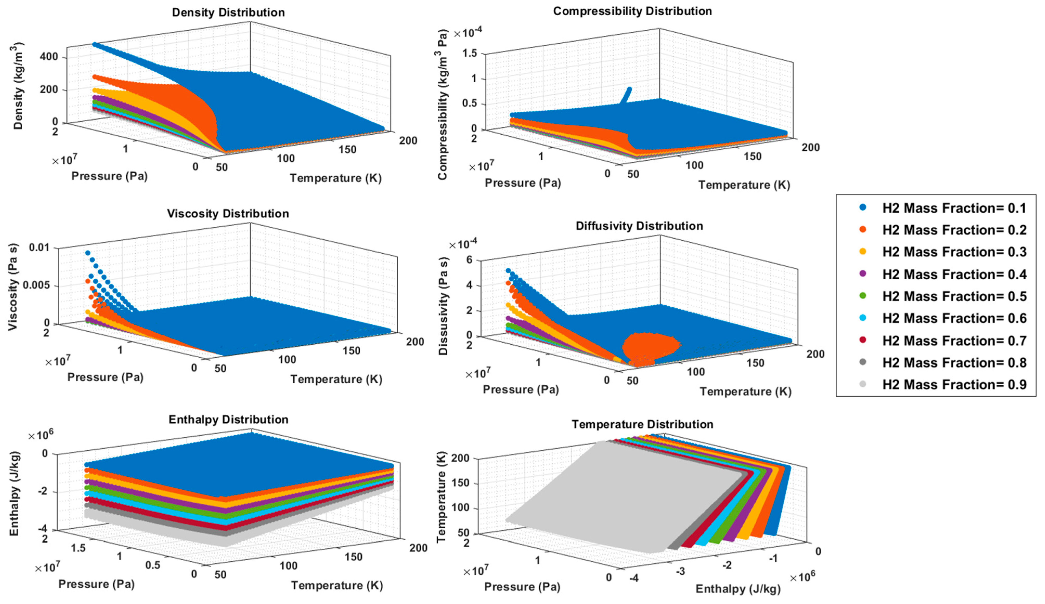
2.3. Training Database

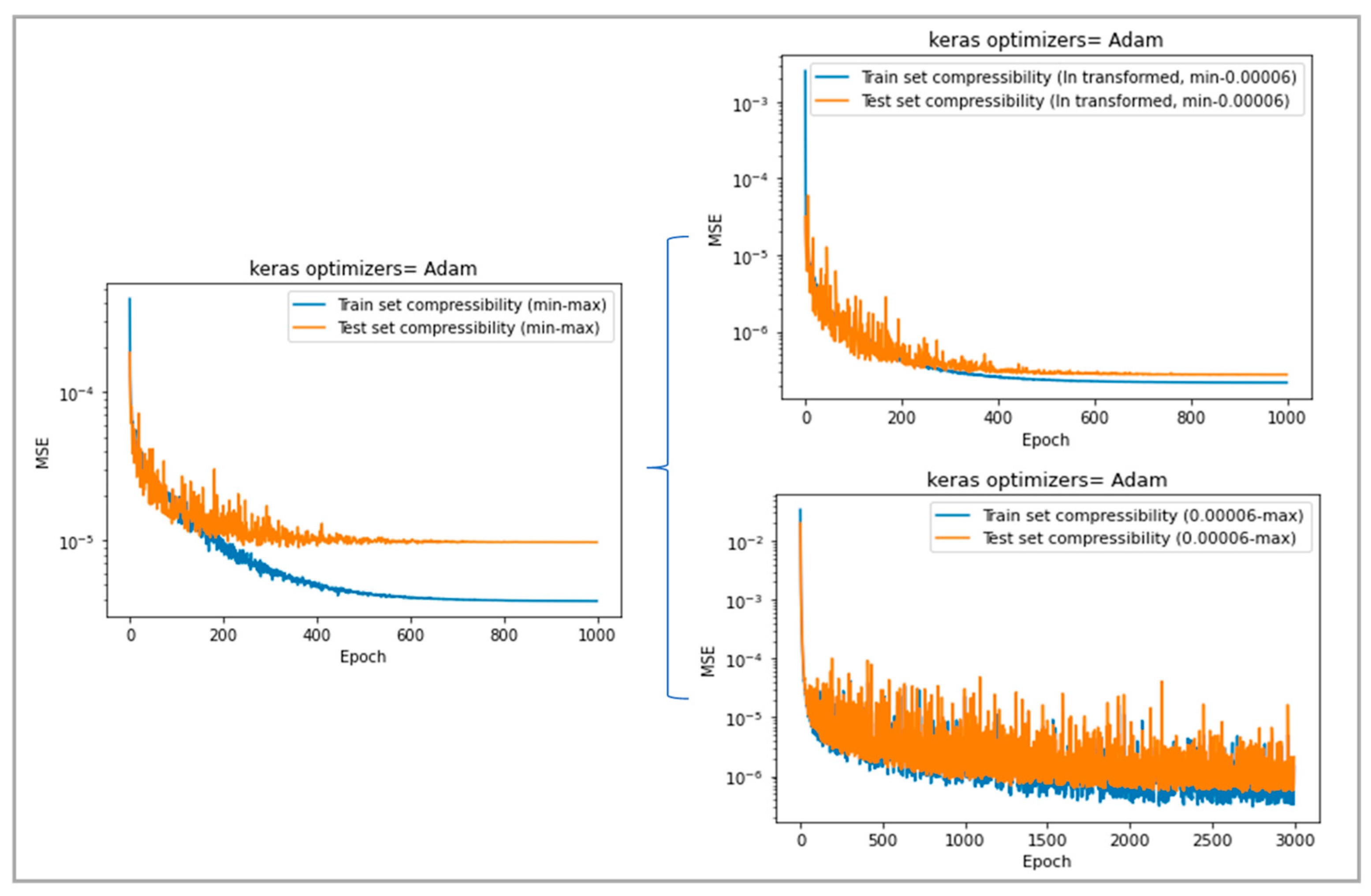
As is shown in

Table 1. List of inputs used for predicting output values.

Inputs		Outputs
Variable Symbol (Code Name)	Definition [Units]
$Y_{H2} \left(Y\right)$	Fuel mass fraction [-]	All output variables (except $T$)
$T \left(T\right)$	Temperature [K]	All variables (except $T$)
$p \left(p\right)$	Pressure [Pa]	All variables (except $T$)
$h \left(he\right)$	Enthalpy [J/kg]	$T$

, the considered inputs are composition ($Y_{H2}$), temperature ($T$), and pressure ($p$) for predicting density ($\rho$), viscosity ($\mu$), thermal diffusivity ($\alpha$), enthalpy ($h$), and compressibility ($\psi$). For predicting temperature ($T$) as the output, composition ($Y_{H2}$), pressure ($p$), and enthalpy ($h$) are considered as inputs. The full definitions and units of the outputs are shown in

Table 2. List of output properties with their definitions and units.

Variable Symbol (Code Name)	Definition [Units]
$\rho \left(rho\right)$	Density [$\mathrm{k}\mathrm{g}/{\mathrm{m}}^3]$
$\mu \left(mu\right)$	Viscosity $[\mathrm{P}\mathrm{a} \mathrm{s}]$
$\alpha \left(alpha\right)$	Thermal diffusivity [$\mathrm{P}\mathrm{a} \mathrm{s}$]
$h$ $\left(he\right)$	Specific enthalpy: $h=sie+p/\rho$ [$\mathrm{J}/\mathrm{k}\mathrm{g}$]
$\psi \left(psi\right)$	Compressibility $\psi =1/\left(ZRT\right) [\mathrm{k}\mathrm{g}/({\mathrm{m}}^3 \mathrm{P}\mathrm{a}\left)\right]$
$T \left(T\right)$	Temperature $\left(\mathrm{K}\right)$

.

In order to generate data, we use the same OpenFOAM library for real fluids that is also implemented in the full original CFD solver. The generated dataset contains 250,000 points, obtained by discretizing the selected temperature and composition ranges with 50 levels each, and the pressure range with 100 levels. In general, the range of each input variable is chosen based on the CFD test case. In the current work, we first consider a large data range where $T$ is between 70 and 200 K, $Y_{H2}$ is between 0 and 1, and $p$ is between 10 and 200 bar. A reduced, or adapted, data range in which $T$ ranges from 70 to 170 K, $Y_{H2}$ from 0 to 1, and $p$ from 50 to 150 bar will also be considered for the final application.

In this specific test case, the properties exhibit highly nonlinear distributions. Consequently, various data transformations are experimented with to enhance network performance. Figure 2 illustrates that the data distributions for enthalpy and temperature are notably smoother, indicating fewer challenges in training these specific properties.

2.4. Model Training

As training tools, Keras and Tensorflow libraries are used, which are open-source libraries that provide a Python interface for NNs. To effectively train a network, data featuring properties relevant to the main problem are required, such as consistent thermophysical properties.

Precision in tuning or optimizing parameters poses a challenge. Hyperparameters, especially learning rate (α), play a crucial role, impacting computational cost, execution time, and network structure. The learning rate is vital in minimizing the loss function during backpropagation, where it iteratively updates biases and weights in hidden layers. This process, involving multiplying the learning rate by the output error of neurons, continues until an acceptable error is achieved for the specified data in each iteration, influencing prediction accuracy and generalization capability.

In the following, all the methods tested to improve the efficiency of the network are elaborated. For all the properties, the min–max scalar is applied for inputs and outputs to facilitate training. As mentioned before, ReLU is considered as an activation function. The optimizer algorithm is Adam, and the loss metric is the mean squared error (MSE). The final values of other hyperparameters like hidden layer size, epochs, and batch size are obtained by experience for each output parameter.

Table 3. Main hyperparameters chosen to train deep networks using Keras library.

Output (Applied Min-Max Scalar)	Inputs (Applied Min-Max Scalar)	Hidden Layer Size	Activation Function	Solver	Learning Rate	Loss Metrics	Epochs	Batch-Size
$rho$$, mu$$, alpha$$, h$$e, psi$	$Y_{H2}, T, p$	100 × 100	ReLU	ADAM	0.0015	MSE	1000	256
$T$	$Y_{H2}, p, he$	100 × 100	ReLU	ADAM	0.0015	MSE	1000	256

reports the number of epochs and the loss metrics for each output parameter. The learning rate is 0.0015, the batch size is 256, and the hidden layer size is considered 100 × 100 for all of the outputs. The influences of choosing different hyperparameters to train the network can be seen in Figure 3 and Figure 4. As is shown in Figure 3, by increasing the number of epochs the relative error decreases for the density, but for a greater number of epochs there will be no change, and also it is likely to end up in overfitting. Also, the effects of using different learning rates are shown in Figure 4. A good way of choosing the hyperparameters is to use previously tested ones, or by experience.

The training algorithm aims to minimize the sum of square errors [27]. This implies that the training minimizes absolute errors across all MLP outputs, regardless of relative errors. However, upon closer examination, as an example, within the compressibility output value range (1.12 × 10⁻⁶–1.18 × 10⁻³ kg/(m³ Pa)), as visible in Figure 5 concerning large data range, it becomes evident that relative errors are notably high, reaching up to 100% at certain points. It is crucial to note that these suboptimal outcomes do not necessarily indicate inadequate MLP training. Instead, they underscore the importance of selecting an appropriate indicator of MLP performance. The substantial relative errors for smaller target outputs could significantly impact the application of MLPs in real simulations [27].

For instance, in our model, temperature serves both as an input and as an output. A substantial relative error in temperature propagates errors in calculating other variables, leading to rapid divergence after a few time steps due to the cumulative effect. To mitigate this, it becomes imperative to diminish the prediction errors of the NN for outputs with small magnitudes. One viable approach is to partition the data into ranges and train the network separately for each output within those ranges.

As illustrated in Figure 5, for the compressibility values within the full dataset range of 1.12 × 10⁻⁶–1.18 × 10⁻³ kg/(m³ Pa), certain points, despite multiple attempts to optimize performance, exhibit relative errors reaching up to 100%, as already mentioned, on the small-value side. However, the objective is to achieve the least relative error. To address this, the data are split into two ranges: the first encompasses 90% of the data, and the second covers the remaining 10%. A log transformation is employed before scaling the data within 0–1 in the first sub-range (1.12 × 10⁻⁶–6 × 10⁻⁵ kg/(m³ Pa)). By normalizing the input and output parameters according to their respective characteristics, we can optimize the learning process, resulting in more efficient predictions and improved overall performance [31]. Also, the logarithmic distribution accommodates the specific characteristics and value ranges associated with output parameters, contributing to enhanced model performance and accuracy [31].

In addition, from the learning curves which are shown in Figure 6, the higher efficiency of this split approach can be seen. Learning curves serve as a frequently employed diagnostic tool for algorithms that iteratively learn from a training dataset. Throughout the training process, the model’s performance is assessed on both the training dataset and a separate validation dataset. The ultimate objective is to achieve a well-fitting model, indicated by a training and validation loss that decreases and stabilizes with minimal disparity between the final loss values. Typically, the model’s loss will be lower on the training dataset than on the validation dataset. Consequently, a gap is expected between the learning curves of training and validation losses, like the curve related to the first range of compressibility, which is shown in Figure 6, but not too much loss, like the curve related to the whole range of compressibility. So, for compressibility after data splitting, the curves related to two different ranges show the training development. An unrepresentative dataset in a specific domain often arises when a dataset’s sample size is insufficient relative to another dataset. An example of this behavior is the curve of compressibility in the second range (6 × 10⁻⁵–1.17 × 10⁻³ kg/(m³ Pa)) in Figure 6, in which the oscillations of the loss show that the training dataset is unrepresentative, which means that it does not provide enough information for effective learning in comparison to the validation dataset used for evaluation [32,33].

However, this approach poses concerns for inference, as there are no predefined criteria for guessing a priori the range of interest. While the analytical thermophysical library of OpenFOAM could be utilized within the CFD solver to guess the output value and make the choice before starting each solver loop, this is a heavy calculation; therefore, it cannot be considered as a general method. Another possibility is using information provided by NN models from a previous timestep, but finding a consistent criterion for subsequent iterations and time steps proves challenging. Another approach would be calling several NNs per cell to begin with, as mentioned in reference [27], in which the training data were clustered into 400 subdomains, and each subdomain was fitted by an individual MLP. Data clustering using the K-mean method, which is a non-supervised clustering algorithm, was performed by Xi Chen et al. [34]. Consequently, this method is set aside, and an alternative approach involving the use of a single network for each property is adopted for the present CFD test case. In essence, for the accuracy and stability of the overall solution algorithm, it has been found that it is easier to have just one network for each property, but with careful selection of the range needed.

As depicted in Figure 7, the relative error consistently meets less than 1% for each variable in the selected reduced range. This successful outcome is observed across density, compressibility, diffusivity, and viscosity. Here, the logarithm transformation is applied, together with the adapted data range close to the needs of the CFD test case (detailed in Section 3). Temperature and enthalpy result in low values of relative errors without logarithm transformation. An essential lesson learned from experience is the careful selection of input and output ranges, particularly those proximate to the test case where the modules will be implemented. In these modules, various data manipulations such as min–max scaling and log transformation are performed. The interplay of these data treatments hinges on the chosen min–max values. Therefore, the judicious selection of a suitable range for training proves pivotal to the overall performance of the network in the following implementation step within the OpenFOAM framework.

2.5. Implementation of NN Models in OpenFOAM

In this study, ML is used to estimate changes in the thermodynamic properties of fluids during the numerical simulation of injection in modern fuel systems and to create surrogate models for two-phase flow predictions. To accomplish this, an NN is established for each fluid property and trained using data derived from dedicated codes, such as 0D thermodynamic simulation models. In the realFluidReactingNNFoam solver, evaluations via Python-trained NN models replace direct evaluations via the original thermophysical libraries for each thermophysical and transport property. To achieve the implementation of the NN models in OpenFOAM, the “Neural Network Inference in C made Easy” (NNICE) code is employed for inferences [35]. NNICE is a simple C++ library designed to provide NN inference capabilities without the complexities associated with compiling traditional ML library C++ APIs. Initially developed for seamless integration into 3D CFD codes, this library is utilized in scenarios where calls to NNs are made in a constrained parallelization environment [35].

Real-fluid thermodynamics and transport are integrated into a solver which utilizes the PIMPLE algorithm. This algorithm uses a pressure-based segregated approach that combines elements of both SIMPLE and PISO methods [2]. To tackle severe pressure and velocity oscillations, a modified reactingFoam solver in OpenFoam is used, called realFluidReactingFoam, which includes a modification of the pressure equation to include linear formulations of density and changes in the frequency of updates of enthalpy and species [24]. This solver with a direct evaluation of real-fluid properties will be considered as the reference.

In the following, a description of the overall CFD solution algorithm is provided, focusing on the points where properties need to be evaluated, and therefore also when NN inference replaces direct evaluation.

• In the initialization stage, $\left(Y_{H2},T,p\right)$ fields are read from dictionaries and values are used to infer each fluid property through Python-trained NN models via NNICE.
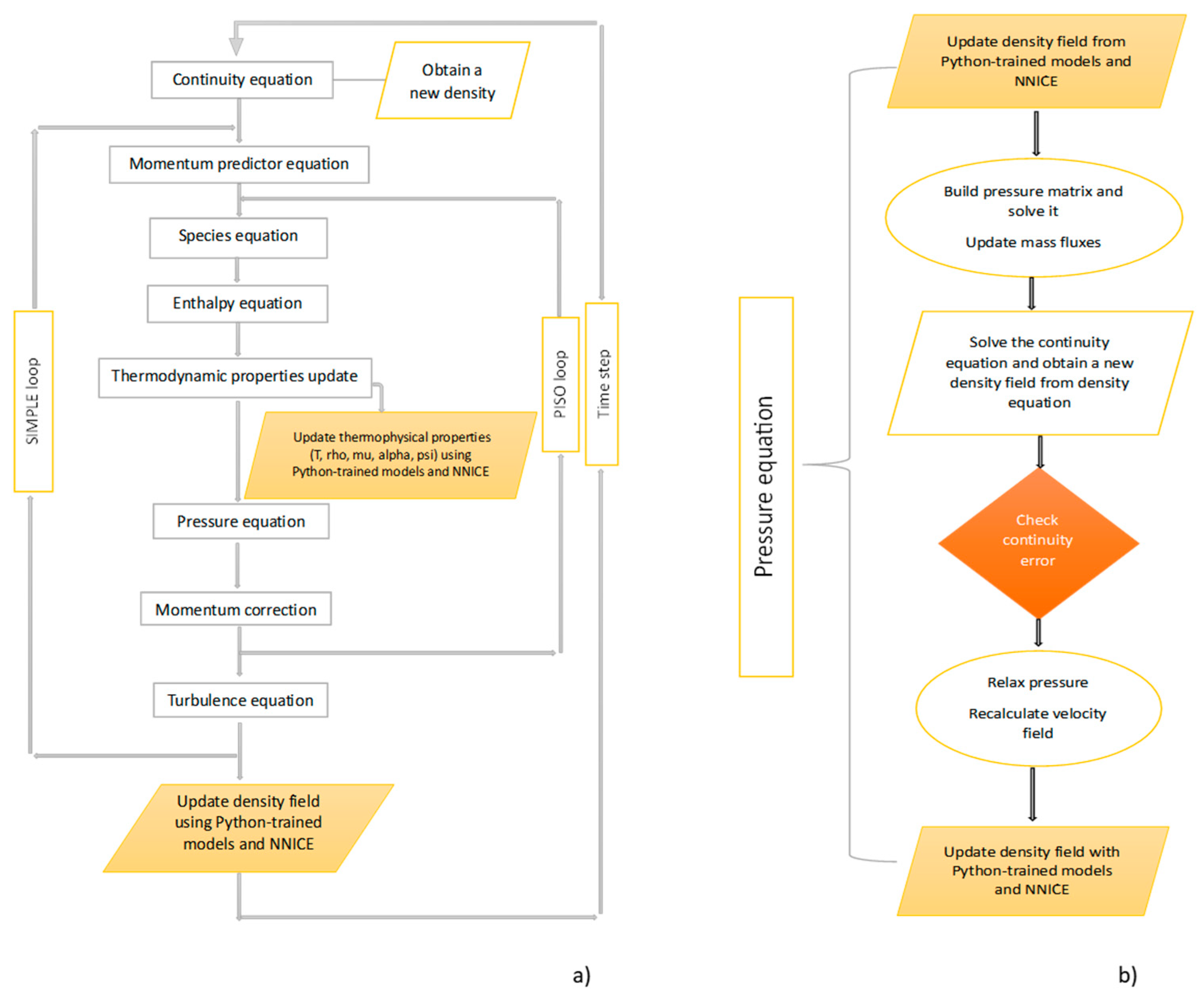
• Then, as shown in the flow chart in Figure 8, at the beginning of a time step, the continuity equation is first solved, and the PIMPLE iteration begins with the momentum predictor step.
• By entering the PISO loop, the species and energy equations are solved. Then, the thermodynamic properties, inferred through the Python-trained NN models with NNICE, replace the original thermo.correct() OpenFOAM function call. In more detail, temperature $T$ is first retrieved after the enthalpy equation is solved using $\left(Y_{H2},p,h\right)$ information; then, all other properties (density $\rho$, viscosity $\mu$, thermal diffusivity $\alpha$, and compressibility $\psi$) are updated using the most recent values of $\left(Y_{H2},T,p\right)$.
• Other inferences are then needed inside each PISO loop. Density is first updated with the corresponding NN model before the pressure equation is solved (details of the pressure equation can be found in Figure 8b). Afterwards, density is explicitly updated, solving the continuity equation, and, after checking the continuity error, the velocity field is updated.
• The last step with the PISO loop concerns a new recalculation of the density field via its NN model.
• Outside the PISO loop, turbulence equations are solved, but no additional inferences are needed there. In addition, in this paper we do not include a turbulence model and assume a laminar flow to show the application of the ML method in OpenFOAM.

2.6. CFD Case Setup

The assessment of the numerical framework is carried out on a cryogenic two-species mixing layer under a transcritical state, which incorporates liquid oxygen (LOX) and gaseous hydrogen (GH2). The case study has already been considered by many researchers, and serves as a well-known benchmark test [2,6,36,37,38,39,40,41,42].

Specifically, we analyze a two-dimensional mixing layer with an injector lip that divides streams of liquid oxygen (LOX) and gaseous hydrogen (GH2), both at supercritical pressure. As shown in Figure 9, this setup serves as a general representation of a cryogenic coaxial injector, where a central dense oxygen jet interfaces with high-speed coaxial hydrogen flow, creating conditions for effective control mixing and flame stability in actual rocket engines [41].

The simulation setup involves an injector lip with a height (h) of 0.5 mm, segregating high-speed gaseous hydrogen (GH2) in the surroundings from dense liquid oxygen (LOX) in the center. A two-dimensional layout is considered. The area of interest of the computational domain spans 15h in the axial direction and 10h in the transversal direction. An additional 15h in the streamwise region serves as sponge layer, designed to mitigate pressure oscillations arising from the outlet. For this study, a relatively coarse mesh is employed with a uniform grid spacing such that h/∆x = h/∆y = 20. The specified resolution is applied up to 15h in the x-direction and extends to 2.5h on both sides of the lip center in the y-direction. The remaining downstream section (from 15h to 30h) of the domain undergoes stretching in the axial direction with a global expansion ratio of 10 [2]. The boundary conditions and computational domain are based on the description provided in [41], but unlike the original benchmark description, no turbulence modelling is employed. As a matter of fact, the present calculations are not meant for assessing model accuracy, but for proving the effectiveness of the NN approach for the fast evaluation of real-fluid properties. Therefore, direct numerical simulation, not including a turbulence model with a relatively coarse grid, makes the test case even stronger and more discerning.

At the injector lip, we implement an adiabatic no-slip wall condition, while the top and bottom boundaries are treated as adiabatic slip walls. Furthermore, we apply a Dirichlet pressure boundary condition at the outlet [2].

As discussed in reference [2], regarding the time discretization, a first-order Euler scheme is applied, while second-order accurate Gauss limited linear schemes are employed for both advection and diffusion.

3. Results and Discussion

This paper extensively explains the development of a model that seamlessly combines a real-fluid model (RFM) with a NN. In terms of surrogate models for approximating thermodynamic functions, NNs demonstrated good performance in predicting properties as functions of pressure, temperature, and mass fractions of a two-component mixture. When used in simulations, since NN regression requires minimal time during evaluation, the computational cost is small. On the other hand, the only alternatives are either evaluating complex thermodynamic models through the RFM, which is rather demanding on the fly, or performing interpolations from tables, the latter being the only practical way in complex cases. However, tables have a large storage footprint and become very cumbersome as the interpolation dimensionality increases (interpolating data among pressure, temperature, and the mass fractions of multiple components) [18,31]. Therefore, the NN seems to be a very attractive option, as the trained network has a size of KBs, which is over a thousand or million times smaller than a table. A further application where the NN can be used is in the development of surrogate models that can be trained using existing, validated data. In the current demonstration case, networks with two hidden layers and 100 neurons each can describe properties as a function of pressure, temperature, and mass fraction adequately well for a LO2/GH2 transcritical mixing layer. It is important to mention that training for a single vector output network takes about 30–60 min (depending on the number of epochs). Its evaluation happens instantaneously—much faster than any simulation could produce.

Another noteworthy aspect is the remarkable versatility of ML. The methods discussed here, even when employed in tandem with simulations, exhibit flexibility in terms of input types. ML can effectively handle diverse forms of data presented in suitable formats. It is crucial to emphasize that this work does not assert to have exhaustively explored the full potential of ML. Admittedly, there are numerous avenues for integrating ML, given its expansive range of techniques adaptable to a multitude of problems. It is only very recently that such ML techniques have begun to be explored in the context of multiphase flows [7].

The open-source code OpenFOAM-v2112 is employed to build distinct solvers, whose results and performance are then presented and discussed. Specifically, such CFD model variants are termed as follows:

• The original CFD model is referred to as realFluidReactingFoam solver. As already explained, it is a real-fluid pressure-based multi-species solver using PR-EoS and Chung models with nonlinear mixing rules coded in OpenFOAM [2,7,24,42].
• The second CFD model is referred to as realFluidReactingNNFoam_1 which adopts a NN approach (referred to here as NN_1 variant) wherein Python-trained NN models and NNICE inference are used to replace original calculations through the RFM.
• The third CFD solver is referred to as realFluidReactingNNFoam_2, which is similar to the second model, but incorporates log transformations for density, compressibility, viscosity, and thermal diffusivity to achieve target accuracy criteria (referred to here as NN_2 variant).
• The last model is referred to as realFluidReactingNNFoam. It is like the previous one, but uses an adapted data range, which means that the data range for training is chosen to be as close as possible to the case study needs to improve network accuracy (referred to here as NN variant).

We start by showing in Figure 10 comparison of the results obtained at 0.1 ms by the codes listed above, namely, the NN variants vs. the original code (realFluidReactingNNFoam_1, realFluidReactingNNFoam_2, realFluidReactingNNFoam, and the reference realFluidReactingFoam). Contours are shown for H₂ mass fraction, temperature, velocity, and density at 0.1 ms. Overall, all fields appear reasonable, and the three ML variants have similar features compared to the original code. Of course, no exact correspondence can be expected, as each simulation produces its own instantaneous results. However, by further scrutinizing these results, it is shown that the first model variant (NN_1) starts generating noisy fields for temperature, velocity, and density, which are attributed to insufficient ML model accuracy. The second variant (NN_2), with transformed input variables, improves the velocity field quality but does not improve other fields. Conversely, the final model variant (NN) preserves clean and smooth fields for all quantities.

The primary objective of this work is to demonstrate the impact of employing NN methods in enhancing RFM simulations by substituting the NN algorithm. Considering the final and more accurate solver version, named realFluidReactingNNFoam, which as explained uses a tailored dataset for training, the results reported in

Table 4. Summary of realFluidReactingNNFoam speed-up vs. realFluidReactingFoam measured on 0.1 ms of physical time and one compute node with 20 cores. (Note that speed-up factors are calculated as the ratio of the time taken by the original code and the time taken by the NN code).

Solver	Total Execution			Iteration
	Time (s)	Speed-Up	Total Number of Iterations	Time/Iter (s/Iter)	Speed-Up
realFluidReactingFoam	511,096	1	200,550	2.548	1
realFluidReactingNNFoam	179,317	2.850	523,200	0.343	7.5

show that the code based on NNs is about 3 times faster for total execution time, and about 7.5 times faster on a time-step basis. This performance is measured considering 0.1 ms of simulated physical time on one compute node with 20 cores, as the test case is not very large in terms of mesh size, to avoid including scalability aspects related to node communication. The tolerances for solving governing equations are kept the same, and in particular 1 × 10⁻⁸ is used for the velocity field, which is quite strict. The NN version of the code requires some more iterations per time step to reach convergence, so although more iterations are needed in general, each one is much faster. Further work can be completed on further improving the accuracy of NN models and optimizing the overall code coupling so that the number of iterations does not increase to obtain an even better speed-up, but the current result already appears promising.

To assess the simulations, result quality comparisons with those from the original approach proposed in [2,25] are presented. Figure 11 shows a scatter plot of mixture temperature vs. hydrogen mass fractions for an instantaneous field at 1 ms, which based on the low speed stream velocity (30 m/s) corresponds already to four flow-through times (FTT) over a distance of 15 h (cf. Figure 9). The NN solver reproduces exactly the thermodynamic states of the reference model, without any appreciable discrepancies.

The corresponding instantaneous fields for H₂ mass fraction, temperature, velocity, and density at 1 ms are shown in Figure 12 for the NN solver realFluidReactingNNFoam and the original solver realFluidReactingFoam. The current numerical solution effectively captures the three prominent vortical structures in the velocity fields, anticipated within x/h = 10, along with the steep density gradient. Kelvin–Helmholtz mechanisms initiate the formation of the initial eddies in the mixing layer, downstream of the lip, prominently on the hydrogen side. These structures, due to interfacial instabilities, contribute to the development of thicker vortices in the oxygen stream [2]. The results of the NN solver are in good agreement with those obtained by the direct RFM solver. These findings showcase the proficiency of the current numerical NN-CFD framework in managing mixing processes involving real-fluid thermodynamic and transport properties under transcritical conditions under the assumption of frozen temperature [26].

Additionally, as a further assessment, a quantitative comparison of statistics collected over time for axial velocity, temperature, and density are presented in Figure 13. These transverse profiles of mean and fluctuating root-mean-square statistics (rms) are obtained by time-averaging instantaneous fields from 1 to 4 FTTs, and are taken at various axial locations, namely at x/h = 3, 5, and 7. Overall, there is very good agreement with the reference trends provided by the realFluidReactingFoam solver.

4. Conclusions

This paper presents a comprehensive exploration of the integration of NN models within the RFM approach for efficiently simulating complex thermodynamic functions in CFD code for a non-evaporating binary mixture under transcritical conditions. The study demonstrates the efficiency of NNs as surrogate models, emphasizing their ability to approximate complex thermodynamic properties with very affordable training times compared to traditional dataset derivation, and significant savings during CFD runtime. The paper highlights the advantages of using NN models in CFD simulations, where computational costs, though present during evaluation, are notably smaller than the original method using direct evaluation from the EoS. The versatility of ML is underscored, particularly in handling various data types and distributions. The work acknowledges the vast potential of ML in the context of multiphase flows and suggests numerous avenues for further exploration. The application of the developed NN models in OpenFOAM to simulate a transcritical mixing case reveals the potential of NNs to replace traditional RFM, offering faster execution times and very good fit, as evidenced by contour plots and averaged transverse profiles. The comparison of realFluidReactingNNFoam results with the original realFluidreactingFoam results indicates that, despite the latter requiring fewer iterations, the NN model outperforms in terms of execution time at the same level of solution accuracy.

In summary, the successful application of NNs in conjunction with RFM in simulating real-fluid thermodynamic and transport properties signifies a promising direction for future research in the field of accelerating computational fluid dynamics models. The study opens avenues for exploring the full potential of ML techniques in addressing complex problems related to multiphase flows with more than just two species.

References

1. He, Z.; Shen, Y.; Wang, C.; Zhang, Y.; Wang, Q.; Gavaises, M. Thermophysical properties of n-dodecane over a wide temperature and pressure range via molecular dynamics simulations with modification methods. J. Mol. Liq. 2023, 371, 121102. [Google Scholar] [CrossRef]
2. Rahantamialisoa, F.N.; Pandal, A.; Ningegowda, B.M.; Zembi, J.; Sahranavardfard, N.; Jasak, H.; Im, H.G.; Battistoni, M. Assessment of an open-source pressure-based real fluid model for transcritical jet flows. In Proceedings of the International Conference on Liquid Atomization and Spray Systems (ICLASS), Edinburgh, Scotland UK, 30 August 2021; Volume 1. [Google Scholar]
3. Qiu, L.; Reitz, R.D. An investigation of thermodynamic states during high-pressure fuel injection using equilibrium thermodynamics. Int. J. Multiph. Flow 2015, 72, 24–38. [Google Scholar] [CrossRef]
4. Puissant, C.; Glogowski, M.J. Experimental characterization of shear coaxial injectors using liquid/gaseous nitrogen. At. Sprays 1997, 7, 467–478. [Google Scholar] [CrossRef]
5. Mayer, W.; Tamura, H. Propellant injection in a liquid oxygen/gaseous hydrogen rocket engine. J. Propuls. Power 1996, 12, 1137–1147. [Google Scholar] [CrossRef]
6. Habiballah, M.; Orain, M.; Grisch, F.; Vingert, L.; Gicquel, P. Experimental studies of high-pressure cryogenic flames on the mascotte facility. Combust. Sci. Technol. 2006, 178, 101–128. [Google Scholar] [CrossRef]
7. Rahantamialisoa, F.N.Z.; Zembi, J.; Miliozzi, A.; Sahranavardfard, N.; Battistoni, M. CFD simulations of under-expanded hydrogen jets under high-pressure injection conditions. J. Phys. Conf. Ser. 2022, 2385, 012051. [Google Scholar] [CrossRef]
8. Oschwald, M.; Smith, J.J.; Branam, R.; Hussong, J.; Schik, A.; Chehroudi, B.; Talley, D. Injection of fluids into supercritical environments. Combust. Sci. Technol. 2006, 178, 49–100. [Google Scholar] [CrossRef]
9. Yang, V. Modeling of supercritical vaporization, mixing, and combustion processes in liquid-fueled propulsion systems. Proc. Combust. Inst. 2000, 28, 925–942. [Google Scholar] [CrossRef]
10. Peng, D.Y.; Robinson, D.B. Robinson, A new two-constant equation of state. Ind. Eng. Chem. Fundam. 1976, 15, 59–64. [Google Scholar] [CrossRef]
11. Oefelein, J.C.; Sankaran, R. Large eddy simulation of reacting flow physics and combustion. In Exascale Scientific Applications: Scalability and Performance Portability; Straatsma, T.P., Antypas, K.B., Williams, T.J., Eds.; CRC Press: Boca Raton, FL, USA, 2018; pp. 231–256. [Google Scholar]
12. Soave, G. Equilibrium constants from a modified Redlich-Kwong equation of state. Chem. Eng. Sci. 1972, 27, 1197–1203. [Google Scholar] [CrossRef]
13. PMilan, P.J.; Li, Y.; Wang, X.; Yang, S.; Sun, W.; Yang, V. Time-efficient methods for real fluid property evaluation in numerical simulation of chemically reacting flows. In Proceedings of the 11th US National Combustion Meeting, 71TF-0396, Pasadena, CA, USA, 24–27 March 2019; pp. 1–10. [Google Scholar]
14. Milan, P.J.; Hickey, J.P.; Wang, X.; Yang, V. Deep-learning accelerated calculation of real-fluid properties in numerical simulation of complex flowfields. J. Comput. Phys. 2021, 444, 110567. [Google Scholar] [CrossRef]
15. Ruggeri, M.; Roy, I.; Mueterthies, M.J.; Gruenwald, T.; Scalo, C. Neural-network-based Riemann solver for real fluids and high explosives; application to computational fluid dynamics. Phys. Fluids 2022, 34, 116121. [Google Scholar] [CrossRef]
16. Jafari, S.; Gaballa, H.; Habchi, C.; de Hemptinne, J.C. Towards understanding the structure of subcritical and transcritical liquid–gas interfaces using a tabulated real fluid modeling approach. Energies 2021, 14, 5621. [Google Scholar] [CrossRef]
17. Jafari, S.; Gaballa, H.; Habchi, C.; Hemptinne, J.C.; De Mougin, P. Exploring the interaction between phase separation and turbulent fluid dynamics in multi-species supercritical jets using a tabulated real-fluid model. J. Supercrit. Fluids 2022, 184, 105557. [Google Scholar] [CrossRef]
18. Koukouvinis, P.; Rodriguez, C.; Hwang, J.; Karathanassis, I.; Gavaises, M.; Pickett, L. Machine Learning and transcritical sprays: A demonstration study of their potential in ECN Spray-A. Int. J. Engine Res. 2022, 23, 1556–1572. [Google Scholar] [CrossRef]
19. Brunton, S.L.; Noack, B.R.; Koumoutsakos, P. Machine learning for fluid mechanics. Annu. Rev. Fluid Mech. 2020, 52, 477–508. [Google Scholar] [CrossRef]
20. Maulik, R.; Fytanidis, D.K.; Lusch, B.; Vishwanath, V.; Patel, S. PythonFOAM: In-situ data analyses with OpenFOAM and Python. J. Comput. Sci. 2022, 62, 101750. [Google Scholar] [CrossRef]
21. Maulik, R.; Sharma, H.; Patel, S.; Lusch, B.; Jennings, E. Deploying deep learning in OpenFOAM with TensorFlow. In Proceedings of the AIAA Scitech 2021 Forum, Virtual, 11–15 January 2021; p. 1485. [Google Scholar]
22. Kim, J.; Park, C.; Ahn, S.; Kang, B.; Jung, H.; Jang, I. Iterative learning-based many-objective history matching using deep neural network with stacked autoencoder. Pet. Sci. 2021, 18, 1465–1482. [Google Scholar] [CrossRef]
23. Liu, Y.-Y.; Ma, X.-H.; Zhang, X.-W.; Guo, W.; Kang, L.-X.; Yu, R.-Z.; Sun, Y.-P. A deep-learning-based prediction method of the estimated ultimate recovery (EUR) of shale gas wells. Pet. Sci. 2021, 18, 1450–1464. [Google Scholar] [CrossRef]
24. Rahantamialisoa, F.N.Z.; Gopal, J.V.M.; Tretola, G.; Sahranavardfard, N.; Vogiatzaki, K.; Battistoni, M. Analyzing single and multicomponent supercritical jets using volume-based and mass-based numerical approaches. Phys. Fluids 2023, 35, 067123. [Google Scholar] [CrossRef]
25. Ningegowda, B.M.; Rahantamialisoa, F.N.Z.; Pandal, A.; Jasak, H.; Im, H.G.; Battistoni, M. Numerical Modeling of Transcritical and Supercritical Fuel Injections Using a Multi-Component Two-Phase Flow Model. Energies 2020, 13, 5676. [Google Scholar] [CrossRef]
26. Chung, T.H.; Ajlan, M.; Lee, L.L.; Starling, K.E. Generalized multiparameter correlation for nonpolar and polar fluid transport properties. Ind. Eng. Chem. Res. 1998, 27, 671–679. [Google Scholar] [CrossRef]
27. Ding, T.; Readshaw, T.; Rigopoulos, S.; Jones, W.P. Machine learning tabulation of thermochemistry in turbulent combustion: An approach based on hybrid flamelet/random data and multiple multilayer perceptrons. Combust. Flame 2021, 231, 111493. [Google Scholar] [CrossRef]
28. Gardner, M.W.; Dorling, S.R. Artificial neural networks (the multilayer perceptron)-a review of applications in the atmospheric sciences. Atmos. Environ. 1998, 32, 2627–2636. [Google Scholar] [CrossRef]
29. Bishop, C.M. Neural Networks for Pattern Recognition; Clarendon Press: Oxford, UK, 1995. [Google Scholar]
30. Watt, J.; Borhani, R.; Katsaggelos, A.K. Machine Learning Refined: Foundations, Algorithms, and Applications; Cambridge University Press: Cambridge, UK, 2020. [Google Scholar]
31. Delhom, B.; Faney, T.; Mcginn, P.; Habchi, C.; Bohbot, J. Development of a multi-species real fluid modelling approach using a machine learning method. In Proceedings of the ILASS Europe 2023, 32nd European Conference on Liquid Atomization & Spray Systems, Napoli, Italy, 4–7 September 2023. [Google Scholar]
32. Anzanello, M.J.; Fogliatto, F.S. Learning curve models and applications: Literature review and research directions. Int. J. Ind. Ergon. 2011, 41, 573–583. [Google Scholar] [CrossRef]
33. Witten, D.; James, G. An Introduction to Statistical Learning with Applications in R; Goodfellow, I., Bengio, Y., Courville, A., Eds.; Deep Learning; Springer Publication, 2013, MIT Press: Cambridge, MA, USA, 2016. [Google Scholar]
34. Chen, X.; Mehl, C.; Faney, T.; Di Meglio, F. Clustering-Enhanced Deep Learning Method for Computation of Full Detailed Thermochemical States via Solver-Based Adaptive Sampling. Energy Fuels 2023, 37, 14222–14239. [Google Scholar] [CrossRef]
35. Aubagnac-Karkar, D.; Mehl, C. NNICE: Neural Network Inference in C Made Easy, Version 1.0.0; Computer Software. Available online: https://zenodo.org/records/7645515 (accessed on 16 February 2023). [CrossRef]
36. Zong, N.; Yang, V. Near-field flow and flame dynamics of LOX/methane shear-coaxial injector under supercritical conditions. Proc. Combust. Inst. 2007, 31, 2309–2317. [Google Scholar] [CrossRef]
37. Zong, N.; Yang, V. Cryogenic fluid jets and mixing layers in transcritical and supercritical environments. Combust. Sci. Technol. 2006, 178, 193–227. [Google Scholar] [CrossRef]
38. Oefelein, J.C. Mixing and combustion of cryogenic oxygen-hydrogen shear-coaxial jet flames at supercritical pressure. Combust. Sci. Technol. 2006, 178, 229–252. [Google Scholar] [CrossRef]
39. Oefelein, J.C. Thermophysical characteristics of shear-coaxial LOX–H2 flames at supercritical pressure. Proc. Combust. Inst. 2005, 30, 2929–2937. [Google Scholar] [CrossRef]
40. Oefelein, J.C.; Yang, V. Modeling High-Pressure Mixing and Combustion Processes in Liquid Rocket Engines. J. Propuls. Power 1998, 14, 843–857. [Google Scholar] [CrossRef]
41. Ruiz, A.M.; Lacaze, G.; Oefelein, J.C.; Mari, R.; Cuenot, B.; Selle, L.; Poinsot, T. Numerical benchmark for high-reynolds-number supercritical flows with large density gradients. AIAA J. 2016, 54, 1445–1460. [Google Scholar] [CrossRef]
42. Ningegowda, B.M.; Rahantamialisoa, F.; Zembi, J.; Pandal, A.; Im, H.G.; Battistoni, M. Large Eddy Simulations of Supercritical and Transcritical Jet Flows Using Real Fluid Thermophysical Properties; SAE Technical Paper 2020-01-1153; SAE: Warrendale, PA, USA, 2020. [Google Scholar]
Figure 1. Schematics of NN with one input layer, two hidden layers, and one output layer with U1 and U2 numbers of units, or neurons (a), and typical structure of a neuron showing input weights, bias, and activation function (b).
Fluids 09 00056 g001
Figure 2. Data distribution of outputs consisting of density, compressibility, viscosity, thermal diffusivity, enthalpy, and temperature for different values of hydrogen mass fraction (large data range).
Fluids 09 00056 g002
Figure 3. Representation of the effects of a higher number of epochs on network performance and the values of the relative error.
Fluids 09 00056 g003
Figure 4. Representation of the effects of the usage of different learning rates as important hyperparameters on network performance.
Fluids 09 00056 g004
Figure 5. Comparison of the relative error and the data distribution before (left) and after range splitting (right). A large data range is considered.
Fluids 09 00056 g005
Figure 6. Mean squared error vs. the number of epochs for compressibility before (left) and after range splitting (right). A large data range is considered.
Fluids 09 00056 g006
Figure 7. Representation of actual vs. predicted values, actual vs. relative error, and distribution of density (purple), compressibility (red), thermal diffusivity (green), viscosity (blue), enthalpy (gray), and temperature (orange). Adapted data range. T : 70–170 K; Y H 2 : 0–1; p : 50–150 bar (this model is referred to as NN variant, or final version, in Section 3).
Fluids 09 00056 g007
Figure 8. Extended PIMPLE solution flow chart for the multiphase transport equations with real-fluid properties (a) and pressure equation flow chart (b).
Fluids 09 00056 g008
Figure 9. Schematics of the case geometry and boundary conditions, adapted from [41].
Fluids 09 00056 g009
Figure 10. Instantaneous fields of H2 mass fraction, temperature, velocity magnitude, and density at 0.1 ms for realFluidReactingNNFoam_1, realFluidReactingNNFoam_2, realFluidReactingNNFoam, and realFluidReactingFoam solvers.
Fluids 09 00056 g010
Figure 11. Scatter plot of instantaneous fields of temperature vs. hydrogen mass fractions at 1 ms. NN results obtained with realFluidReactingNNFoam solver.
Fluids 09 00056 g011
Figure 12. Instantaneous fields of H2 mass fraction, temperature, velocity magnitude, and density at 1 ms for realFluidReactingNNFoam and realFluidReactingFoam solvers.
Fluids 09 00056 g012
Figure 13. Transverse profiles of mean (up) and rms (down) x-velocity, temperature, and density.
Fluids 09 00056 g013