Abstract
The purpose of this work is to explore the potential of deep reinforcement learning (DRL) as a black-box optimizer for turbulence model identification. For this, we consider a Reynolds-averaged Navier–Stokes (RANS) closure model of a round turbulent jet flow at a Reynolds number of 10,000. For this purpose, we augment the widely utilized Spalart–Allmaras turbulence model by introducing a source term that is identified by DRL. The algorithm is trained to maximize the alignment of the augmented RANS model velocity fields and time-averaged large eddy simulation (LES) reference data. It is shown that the alignment between the reference data and the results of the RANS simulation is improved by 48% using the Spalart–Allmaras model augmented with DRL compared to the standard model. The velocity field, jet spreading rate, and axial velocity decay exhibit substantially improved agreement with both the LES reference and literature data. In addition, we applied the trained model to a jet flow with a Reynolds number of 15,000, which improved the mean field alignment by 35%, demonstrating that the framework is applicable to unseen data of the same configuration at a higher Reynolds number. Overall, this work demonstrates that DRL is a promising method for RANS closure model identification. Hurdles and challenges associated with the presented methodology, such as high numerical cost, numerical stability, and sensitivity of hyperparameters are discussed in the study.
1. Introduction
Reynolds-averaged Navier–Stokes (RANS) simulations are widely used in scientific research and industrial applications. Due to the nonlinearity of the Navier–Stokes equations, the RANS equations include time-averaged products of the velocity fluctuations—the Reynolds stresses—in addition to the mean velocity components and the mean pressure. In total, the RANS equations thus have six additional unknowns, which are typically combined in the Reynolds stress tensor. To solve the RANS equations, i.e., to simulate a mean flow field, the Reynolds stress tensor has to be modeled, which is also known as the turbulence closure problem. The RANS equations are based on the premise that the entire spectrum of turbulence must be modeled. However, since the large and medium turbulence scales are highly domain- and boundary-condition-specific, the optimal choice of model depends strongly on the problem at hand.
The most common way to model the Reynolds stress tensor is provided by the Boussinesq hypothesis [1], which relates the deviatoric part of the Reynolds stress tensor to the strain rate tensor through the Boussinesq eddy viscosity [2], thus reducing the number of additional unknowns to one. When the Boussinesq hypothesis is employed, an additional model for the eddy viscosity must be chosen, with algebraic, one- and two-equation models available. A popular one-equation model is the Spalart–Allmaras (SA) model [3]. Famous two equation models include the k- and k- models [4]. Menter [5] developed the Menter SST model that utilizes the advantages of the k- and k- models. It is now part of industrial and commercial CFD codes [6]. For many technical flows, the Boussinesq hypothesis is already too restrictive, so more sophisticated turbulence models, such as the Reynolds stress transport model, are frequently used. Depending on the flow configuration considered, one or the other model performs better.
Adapting and modifying models for specific configurations is still an active topic of research. Raje and Sinha [7], for example, developed an extended version of the Menter SST model for shock-induced separation under supersonic and hypersonic conditions. Menter et al. [8] developed a generalized k- model that allows easy adaptation of the turbulence model to new configurations. In these studies, physics-based considerations are used to extend, improve, or generalize the turbulence model. This approach can also be referred to as a knowledge-based approach.
On the contrary, data-driven approaches aim to identify/learn closure fields from high-fidelity reference data [9]. By relating the identified fields back to the mean field quantities, improved closure models can be identified in a purely data-driven manner. Foures et al. use a data-assimilation technique to match a RANS solution to time-averaged DNS fields of a flow around an infinite cylinder [10]. The approach is based on a variational formulation that uses the Reynolds stress term as a control parameter. In subsequent studies, a similar approach is applied based on measured particle image velocimetry (PIV) data [11], for assimilating the flow field over a backward-facing step at a high Reynolds number (28,275) [12]. In parallel, a Bayesian inversion-based data assimilation technique was developed called field inversion [13]. The method is applied, for example, in Refs. [13,14], to identify a spatially resolved coefficient in the k- and Spalart–Allmaras model, respectively, to match the RANS solutions to high-fidelity mean fields. In recent studies, closure fields are identified by assimilating RANS equations to LES, PIV [15], and DNS [16] mean fields using physics-informed neural networks.
The studies mentioned above all apply data assimilation/field inversion methods to identify closure fields or parameters in closure models that lead to an optimal match between the RANS solutions and the high-fidelity data. However, they do not relate the identified fields back to the mean field quantities, i.e., no predictive closure models have yet been identified. This first step of retrieving an optimal or best-fit closure field can be considered as collecting a priori information. Based on the information collected, data-driven approaches typically apply supervised learning algorithms in a subsequent step to determine an improved closure model [17,18]. The quality of the identified models can then be evaluated in an a posteriori analysis.
Machine learning algorithms allow for extracting patterns from data and building mappings between inputs and outputs [19]. Methods that apply machine learning to closure modeling can be categorized into two groups: algorithms that learn from existing turbulence models to mimic their behaviour, and algorithms that learn from high-fidelity data to improve the accuracy of RANS closure models. The former is addressed, for example, by Xu et al. [20], who apply a dual neural network architecture to replace the k- closure model. The inputs of the neural network are composed of local and surrounding information, a concept known as the vector cloud neural network (VCNN) [21]. The latter, machine learning-enhanced closure modeling, is of particular relevance for the present study and is discussed, for example, in Refs. [17,18]. As described above, the studies first identify an optimal closure field, which is then related to the mean field quantities in a subsequent step using a supervised learning algorithm to find an improved closure model in a purely data-driven way.
Supervised learning algorithms require training data that consist of input data points and known true outputs. The majority of the research on applying machine learning to turbulence closure models utilizes supervised learning [22]. However, recent studies have shown a growing interest in utilizing reinforcement learning (RL) techniques for turbulence closure modeling. This shift is somewhat counter-intuitive, as the initial inclination might be to rely on supervised learning due to its established methodologies and frameworks. However, supervised learning cannot be used for problems where the true output is not known, as is often the case with closure modeling [23].
In contrast to existing two-step methods using supervised learning, the present work is concerned with improving closure modeling in a single step based on a reinforcement learning algorithm that does not require the collection of a priori information. As demonstrated by Novati et al., multi-agent reinforced learning (MARL) is a suitable algorithm for closure model improvement [24]. In simplified terms, reinforcement learning is based on an agent (a function) observing its environment (taking input variables), acting (returning an output), and receiving a reward for its actions. The agent tries to choose its actions in a way that maximizes the reward it receives. This approach eliminates the need to provide the algorithm a priori with information that it can learn. Multi-agent reinforcement learning applies multiple agents distributed over the domain.
Reinforcement learning has gained large popularity due to the method’s great success in achieving super human performance in games like Go [25], Dota II [26], and the Atari 2600 games [27]. Moreover, the method has been successfully applied in robotics [28], autonomous driving [29], and non-technical tasks such as language processing [30] or healthcare applications [31]. Despite the success and popularity of the method in other fields, its application in fluid mechanics is limited [32,33].
Most studies on reinforcement learning in fluid mechanics are concerned with flow control, with both numerical [34,35,36,37,38,39,40,41,42] and experimental studies [43,44]. The study by Novati et al. [24] applies reinforcement learning to improve the subgrid-scale (SGS) turbulence modeling of a large-eddy simulation (LES) by learning from DNS data. The spatially distributed agents receive local and global information about the mean flow as state input (observing) and determine the dissipation coefficient of the Smagorinsky SGS model at the cells they are located at (acting). Agents receive a reward based on the difference between the LES solution compared to the DNS reference data. The described framework is successfully applied to different Reynolds numbers and different mesh resolutions. This approach is expanded by Kim et al. [45] by incorporating physical constraints in order to apply the method to wall-bounded flows. Kurz et al. [23] apply a multi-agent RL algorithm for implicitly filtered LES in a similar setup as Novati et al. [24]. Other than Novati et al. [24], they surpass the performance of conventional subgrid-scale models by only relying on local variables utilizing a convolutional neural network architecture. Yousif et al. [46] apply a multi-agent DRL-based model to reconstruct flow fields from noisy data. They incorporate the momentum equations and the pressure Poisson equation and, therefore, create a physics-guided DRL model. Using noisy data (DNS and PIV measurements), it is shown that the model can reconstruct the flow field and reproduce the flow statistics.
The literature reviewed here illustrates both the success of data-driven methods for improving RANS closure modeling and the success of DRL as an optimization method in various domains including fluid mechanics. The idea of the present study is to combine the two successful methodologies and perform data-driven RANS closure modeling with DRL. It should be noted that the objective of this study is not to identify the most effective data-assimilation method. We are aware that other optimization and data-assimilation methods are capable of solving comparable optimization problems. The aim of the present study is to explore the extent to which DRL-based closure models can open up new fields of application for existing RANS turbulence models. Unlike LES, in RANS simulations, the entire turbulence spectrum must be modeled, making the approach very difficult to generalize. RANS turbulence models must, therefore, be selected on an application-specific basis and perform poorly when transferred to other applications.
In the present study, we consider a turbulent jet flow and the Spalart–Allmaras turbulence model, which is known to perform rather poorly for jet flows [4]. Thus, it is a suitable case to investigate the extent to which the closure model can be improved with the DRL algorithm. We introduce an additional source term into the Spalart–Allmaras transport equation that serves as a degree of freedom for the algorithm. The source term allows to modify both the production and dissipation terms and, therefore, allows a very high degree of freedom for the algorithm [47]. However, it is still bound by the transport equation of the SA model. The mean field dependence of this source term is determined by the DRL algorithm. The objective of the DRL algorithm (reward function) is to match the augmented Spalart–Allmaras RANS results with high-fidelity time-averaged LES velocity fields. Inspired by the studies of Novati et al. [24] and Xu et al. [20], a multi-agent approach is used, which augments the turbulence model locally and, thus, allows a model trained on one configuration to be applied to other configurations.
To address numerical difficulties that arise at the interface between the RANS solver and the machine learning-augmented turbulence model, the DRL algorithm is directly integrated into the flow solver, i.e., rewards are only awarded when the machine learning-augmented RANS solver converges. The open-source software package OpenFOAM (version 4.X) is used to solve the RANS equations.
2. Optimization Methodology
The objective of the DRL algorithm is to align RANS solutions with high-fidelity LES reference data. A brief description of the reference data is provided in Section 2.1, followed by the governing equations in Section 2.2. Details of the RANS simulation are given in Section 2.3. Section 2.4 presents the stencil approach that is the core of the optimization setup. Section 2.5 introduces the deep reinforcement learning algorithm, and Section 2.6 discusses the algorithm’s hyperparameter dependence.
2.1. Reference Data
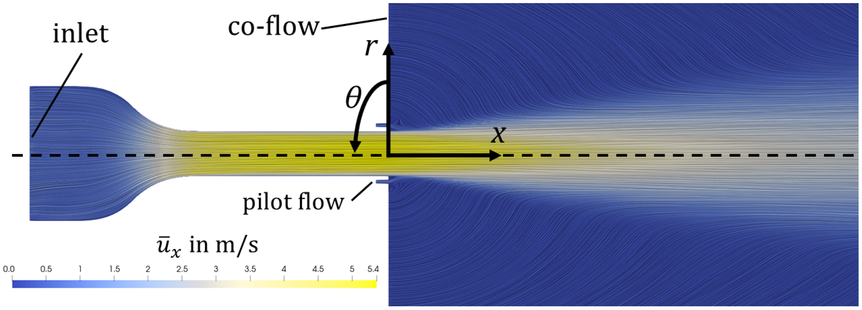
The reference data come from an LES dataset from a turbulent round jet [48,49]. The computational domain is shown in Figure 1. It consists of a converging nozzle, a straight duct, an annular inlet around the nozzle, and a large cylindrical plenum. The geometric configuration represents a jet flame combustor, where, under reacting conditions, fuel is injected at the annular inlet, which is called the pilot flow nozzle. Here, under non-reacting conditions, air is injected at the pilot flow inlet. In total, the domain has three inlets: the main inlet at the converging nozzle, the annular pilot, and the co-flow inlet. The co-flow is used to prevent undesired recirculation and improves numerical stability. Although the boundary conditions and geometry of the setup hold greater technical relevance, the underlying flow fundamentals remain comparable to those of a generic round jet.
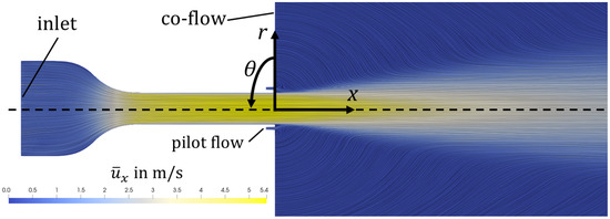
Figure 1.
Axial velocity field and streamlines (visualized using Line Integral Convolution) of a 2D slice through the LES mean field.
The Reynolds number, defined as , is calculated using the duct diameter D, the bulk velocity and the kinematic viscosity . Datasets with Reynolds numbers of 10,000 and 15,000 are considered in this study. To obtain the mean fields, the LES snapshots are time- and azimuthally averaged. For further details on the LES, we refer the reader to the original publication of the data [48,49].
2.2. RANS Equations
Time averaging the incompressible Navier–Stokes equations yields the Reynolds-averaged Navier–Stokes equations:
where denotes the density, p the pressure and the molecular kinematic viscosity. The velocity vector is expressed in cylindrical coordinates, where x is the axial coordinate, r the radial coordinate, and the azimuthal coordinate. The coordinate system is shown in Figure 1. The vector denotes the time-averaged mean velocity and denotes the remaining fluctuating part such that . The Reynolds stress tensor introduces six additional unknowns that must be modeled in order to solve the RANS equations as a boundary value problem. This modeling requirement is known as the turbulence closure problem. An approach to modeling is the Boussinesq hypothesis [1], which relates the deviatoric part of the Reynolds stresses to the strain rate tensor through a turbulent viscosity, known as the eddy viscosity :
where denotes the turbulent kinetic energy and is the identity tensor.
Using the Boussinesq model leaves one unknown, the eddy viscosity, for which, again, several models are available in the literature. Here, we focus on the Spalart–Allmaras turbulence model [3]. In this model, the eddy viscosity is modeled with one transport equation. Spalart and Allmaras [3] follow the formulation of Baldwin and Barth [50] and introduce as a transported quantity that is defined by . The function is designed so that behaves linearly in the region near the wall, which is desirable for numerical reasons [3]. The transport equation is given by:
where , , , and are model constants, is the molecular viscosity, is the density, d is the wall distance, is a production term, and is a near-wall inviscid destruction term. For more details on the Spalart–Allmaras terms and model constants, see [3,51,52].
To introduce a degree of freedom for the DRL algorithm, we add an extra source term into the transport equation. The source term is modeled as a function of the mean field that is identified by the DRL algorithm, which is introduced in the next chapter.
The choice of the Spalart–Allmaras model arises from its reputation for robust numerical stability [4]. Moreover, it has been used in a range of data-driven and machine learning closure model studies as mentioned in Section 1 [12,13,14,53]. However, it is essential to note that the model is known for its poor performance on jet flows (see Tables 4.1 and 4.4 in Ref. [4]). Thus, the Spalart–Allmaras model applied to a jet flow is a particularly suitable case for the objective of this study, namely, to investigate the extent to which DRL can extend the scope of a closure model.
2.3. RANS Simulations
The computational domain for the RANS simulations is sketched in Figure 2. Exploiting the axial symmetry of the mean field, the domain only contains the part above the centerline and lies in the x-r plane. The domain is created in a wedge shape with a single cell in azimuthal direction, as typically done for 2D computations with finite-volume methods. To simplify the computational domain, the converging nozzle and the annular pilot flow nozzle are omitted and replaced by inlet surfaces. The main inlet of the domain is placed at the beginning of the straight duct, upstream from the nozzle. The mean field Equations (1)–(3) are solved numerically using the Semi-Implicit Method for Pressure Linked Equations (SIMPLE) solver in OpenFOAM (version 4.X). The velocity boundary conditions for the main inlet and the pilot flow inlet are set to the corresponding LES values. The co-flow inlet uses a uniform fixed-value velocity inlet. The duct wall, the two walls around the pilot flow inlet, and the wall on top of the plenum are no-slip walls. At the outlet surface, the boundary condition for the velocity is set to zero gradient condition. The boundary condition for the pressure is zero gradient for all surfaces except the outlet surface. Here, a fixed value of is set. The boundary conditions for are chosen according to the recommendations in Ref. [52]. The mesh is a structured hexahedral mesh generated using the blockMesh utility [54] and simpleGrading [54]. For the training of the algorithm, it is of great importance to choose a mesh that is as coarse as possible. It is, however, crucial to have a numerically converged mesh to make sure that the DRL algorithm is optimizing SA model errors and not numerical errors that are related to an under-resolved mesh. Based on a grid refinement study, employing a mesh size of 11,990 cells was deemed optimal, as further resolution increased by a factor of four showed negligible impact on velocity profiles.
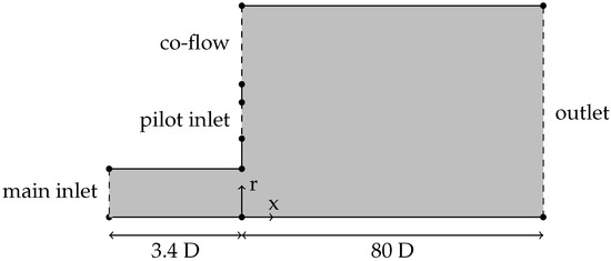
Figure 2.
RANS domain schematic (representation is not true to scale).
2.4. Optimisation Setup Using a Stencil Approach
The objective of the DRL algorithm is to find a function that maps mean flow quantities to the source term in the Spalart–Allmaras transport equation and that minimizes the difference in velocity fields between the RANS and the reference LES mean field:
where stands for an L2-norm. However, the goal of DRL is not only to find an optimal field, but rather to identify a function that maps flow variables to . Since the identified function depends only on mean flow quantities, it can be directly incorporated into the turbulence closure model without the need for further closure equations. The DRL thus performs two steps at once: the search for an optimal closure field and, simultaneously, relating it to flow variables.
The functional structure can be considered as a hyperparameter and its motivation shall be discussed in the following. The most direct way to construct a function would be a local mapping that assigns a value to a set of mean field quantities at each position. However, in order to provide the function with gradient and flow information in the immediate vicinity, the function is constructed in such a way that the flow field of the surrounding region of the target position is used as input. Therefore, the information from the upstream (and downstream) of the flow is also included in the determination of .
We label the surrounding of a target cell as a stencil. Here, we choose a rectangular area with an edge length of and the target cell in the center. However, we stress that the appropriate choice of stencil shape and size depends on the domain dimensions and the Reynolds number of the flow. The algorithm should learn from the significant flow features. The stencil size should therefore be large enough to capture large parts of the shear and boundary layers and geometric features such as steps and edges. The stencil size selected in this study allows one to cover the flow between the duct wall and the centerline, as well as the pilot flow inlet and parts of the nozzle, and, thus, covers key-geometric features within single stencils.
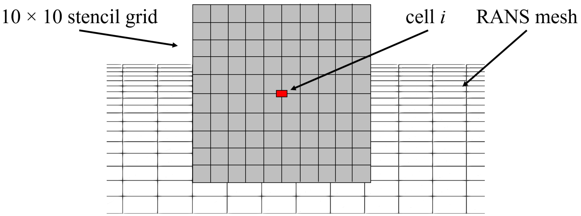
However, the use of the stencil method also presents technical challenges. Typically, numerical grids are non-uniform, so that, depending on the target cell under consideration, different numbers of grid points lie within the stencil region. To overcome this difficulty, the stencil is constructed with equidistant points, and a routine is implemented that interpolates the mean flow quantities from the non-uniform RANS to the equidistant stencil grid. This ensures that the function always receives the same number of input values with the same distance to the target cell. A symbolic representation of the stencil grid on top of the RANS grid is visualized in Figure 3.
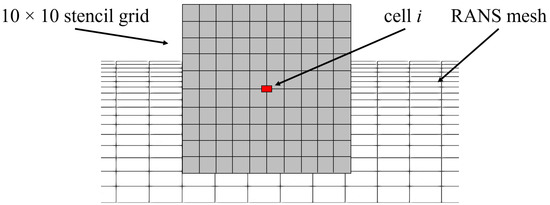
Figure 3.
Symbolic representation of the stencil grid on top of the RANS mesh.
As input for the -function on the stencil grid, we choose the mean axial and radial velocity components and the eddy viscosity as mean flow variables. The values are normalized with 1.2 of their respective maximum value. Normalization is necessary due to the internal architecture of the DRL algorithm, which requires a predefined value range for input and output. Normalization also enables generalizability of the identified -function to other flow conditions that will be discussed later (see Section 3). The factor prevents the clipping of values that exceed the maximum value (internal to the DRL algorithm). Furthermore, the normalized radial coordinate of the target cell is passed to the stencil as an input variable, since it represents a decisive variable for cylinder coordinates and it supplements the algorithm with additional spatial information. It is normalized with its maximum value. One stencil vector, denoted , thus consists of entries: three fields (with entries each) and one scalar. In this study, proved to be a good choice, resulting in 301 input values for the function to be identified by the DRL algorithm. During model training, at every iteration, the stencil vector is constructed and evaluated for each cell of the RANS simulation, resulting in the field required to evaluate the augmented Spalart–Allmaras transport equation, Equation (3).
For target cells that are close to the boundary, the stencil grid extends beyond the domain. To address this, boundary conditions are implemented. Along the centerline (lower boundary), mirrored data points extend beyond the RANS solution domain. Beyond solid walls, zero-velocity data points are appended. Close to the inlet and outlet, the values on the boundary are extended beyond the boundary. This approach ensures that, as the stencil grid surpasses the computational domain, the interpolated data aligns with the specified boundary conditions.
We conclude this section with a discussion of the advantages of the presented approach. The stencil approach divides the large dataset of the entire domain into smaller subsets (the stencil vectors), which presents three advantages. First, each stencil vector can be considered as a training point for the DRL algorithm. Thus, the costs associated with generating training points are substantially reduced in comparison to using the entire mesh as input to the function, since a single RANS simulation provides training points equivalent to the number of cells. Second, the dimension of a single data point for training the -function is significantly reduced. This reduction in dimensionality leads to a reduction in the complexity of the -functional architecture and enables shorter training times. Lastly, and most importantly, the proposed approach enables generalizability, since the algorithm learns from localized flow phenomena instead of the entire domain. Thus, a trained algorithm can be applied to different geometries or flow conditions.
2.5. Deep Reinforcement Learning Algorithm
To identify the -function that leads to a good alignment of the RANS solution with the LES mean field (Equation (4)), deep reinforcement learning is used. Reinforcement learning is based on an agent observing its environment, acting, and receiving a reward for its actions. The agent tries to choose its actions in such a way that it maximizes the reward received. Rewards can, but do not have to, be granted after every action. They can be given after a sequence of actions. According to Sutton and Barto [55], the two most characteristic features of reinforcement learning are trial-and-error search and delayed reward. One episode of training consists of multiple interactions in which the agent observes the state and performs an action. One round of chess, for example, consists of multiple moves. For each move, the agent receives the results of its last actions as a new state. This can be described as a closed-loop system, which is the classical design of RL frameworks.
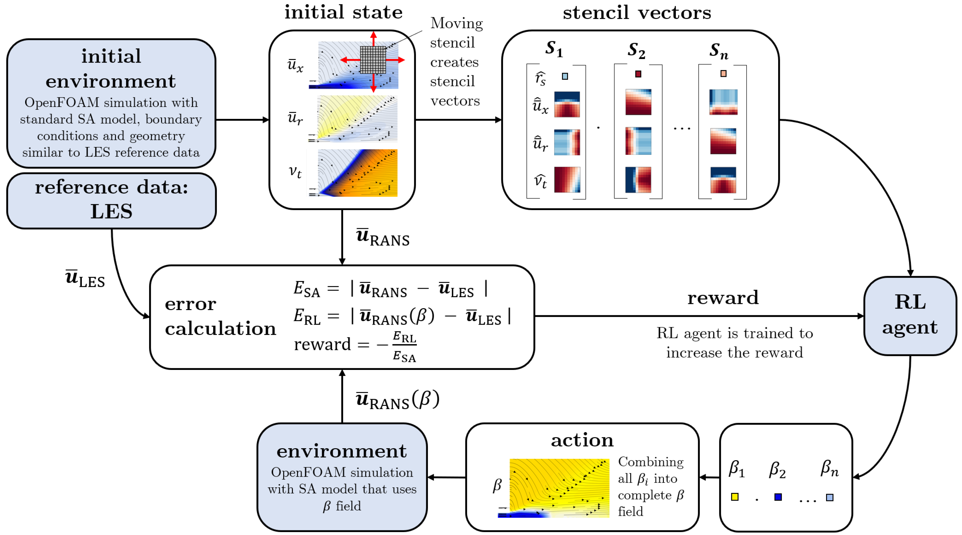
In this work, a simplified single-step open-loop implementation of reinforcement learning is used and is visualized in Figure 4.
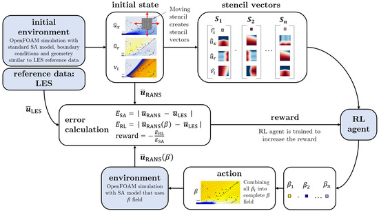
Figure 4.
Optimization methodology showing single-step open-loop reinforcement learning and stencil approach.
First, an initial run of the environment is performed: a RANS simulation with the standard Spalart–Allmaras eddy viscosity model is run until convergence. The resulting velocity and eddy viscosity field are referred to as initial states which determine the reference error
The initial run is just performed once. Subsequently, for each cell, the stencil vector is computed and the reinforcement learning agent applies the function to determine the value at every point. With the complete field, the RANS solver is run for a predefined number of iterations. The resulting mean field allows for the calculation of the distance to the reference data in a predefined range and
The distance to the reference data allows us to define a reward function to be maximized by the DRL algorithm
Dividing the distance to the reference data by the reference error serves as normalization and enhances the transferability of trained agents to new cases. Formulating the function with negative values yields optimal results. After the reward is calculated, it is passed to the agent, together with the stencil vectors and the determined values to train the agent’s algorithm. Depending on how the reward changed with respect to the preceding episode, the agent is trained in order to increase the expected reward. In the next episode, the agent receives the same stencil vectors as in the previous episode and determines new values. The chosen algorithm implements the agent as a neural network [56]. The goal of the algorithm is to maximize the reward (Equation (7)) by finding parameters of the neural network that minimize the error : .
The algorithm presented in this study is referred to as having a single-step open-loop design. Although the function is evaluated multiple times in one episode to compute a value of the source term for each cell in the domain, it is termed a single-step design because only a single RANS solution is processed per episode. The RANS solution with the augmented SA model is used only to compute the reward and is not decomposed again. The subsequent episodes start again with the initial state. Consequently, this approach simplifies the DRL algorithm into an optimization tool.
For the DRL algorithm, we used the proximal policy optimization (PPO) [57]. It was selected because it is known for its good sample efficiency, which means that it can achieve good performance with limited training data, which is a crucial requirement for this work. Additionally, it naturally handles continuous state and action spaces, it has been proven to be applicable in a single-step open-loop configuration [58,59], and it is the most common DRL algorithm used in the context of fluid dynamics [32,60]. To implement the PPO algorithm, we used the open-source package tensorforce by Kuhnle et al. [56]. For further implementation details, refer to Refs. [56,57].
To evaluate the effectiveness of the algorithm, we also computed the relative error reduction RER of the error achieved with the trained model compared to the initial state
The method introduced in this work shares similarities with other publications, which are outlined below. In the present work, we use the local surrounding of a point as input data, comparable to the methods of Xu et al. [20] and Zhou et al. [21]. We combine this approach with the concept of multi-agent reinforcement learning that was also used by Novati et al. [24] and Yousif et al. [46]. Our method is configured in an open-loop design that is comparable to those of Viquerat et al. [58] and Ghraieb et al. [59]. The approach presented in this study does not include rotational invariance. However, it can be easily implemented, similarly to other studies [21,24].
2.6. Hyperparameters
The PPO implementation of the DRL algorithm in the tensorforce library has multiple hyperparameters. Applying the algorithm with the default values did not lead to successful results, and selecting appropriate hyperparameters turned out to be crucial to achieving well-performing models. In our analysis, we identified three influential hyperparameters for which non-default values were required to achieve large error reductions: baseline optimizer (BO) learning rate, batch size, and regularization.
The DRL algorithm uses two neural networks. They are termed the policy network and the baseline network. The policy network determines the output value of and is called the function in this work. The baseline network estimates so-called state values that are required for training the policy network [56]. The first influential hyperparameter is the learning rate of the baseline optimizer (BO), which determines the learning rate of the optimizer that updates the parameters of the baseline network [56]. By default, the tensorforce library uses a BO learning rate of . The second influential hyperparameter is the batch size. It determines how many training points (stencil vectors) are used in a batch to update the agent’s parameters. For this hyperparameter, there is no default setting as it is very data specific. It has to be set manually. The third influential hyperparameter is the L2 regularization coefficient. It penalizes large network weight values. By default, the tensorforce library uses no L2 regularization.
A hyperparameter study was conducted to determine a well-functioning model. The results are shown in Table 1 and Table 2. The tables show that well-performing models are in two groups: The first group is characterized by small batch sizes of ≈1000, a disabled L2 regularization, and larger BO learning rates ≈ (Table 1). The second group is characterized by larger batch sizes of ≈3000, an L2 regularization of 0.01, and small BO learning rates of ≈ (Table 2). From this, we conclude that the algorithm performance is very sensitive to hyperparameters. Small changes can cause drastic performance losses. As using default hyperparameters does not result in a functioning model, hyperparameter studies are necessary.

Table 1.
Hyperparameter study with batch sizes , BO learning rates , and L2 regularization = 0.0, showing the relative reduction in errors .
Table 2.
Hyperparameter study with batch sizes , BO learning rates , and L2 regularization = 0.01, showing the relative errors .
3. Results
In this section, we first present the results of the RL algorithm applied to the jet at Re = 10,000. Thereafter, we present results of the trained network applied to a higher Re case to test the extrapolation capabilities.
3.1. Model Training and Validation for Re = 10,000
The objective of the RL algorithm is to minimize the error, which consists of the distance between LES and RANS velocity field (Equation (6)). We used the optimal hyperparameter determined from the hyperparameter study conducted in Section 2.6 in order to achieve the lowest error value. The results of the RL model were compared to the simulation based on the standard SA turbulence model without the source term . The deviation of the standard SA model from the LES mean fields gave an error value of . After model training, the error was reduced to , which corresponds to a relative reduction in error (Equation (8)) of .
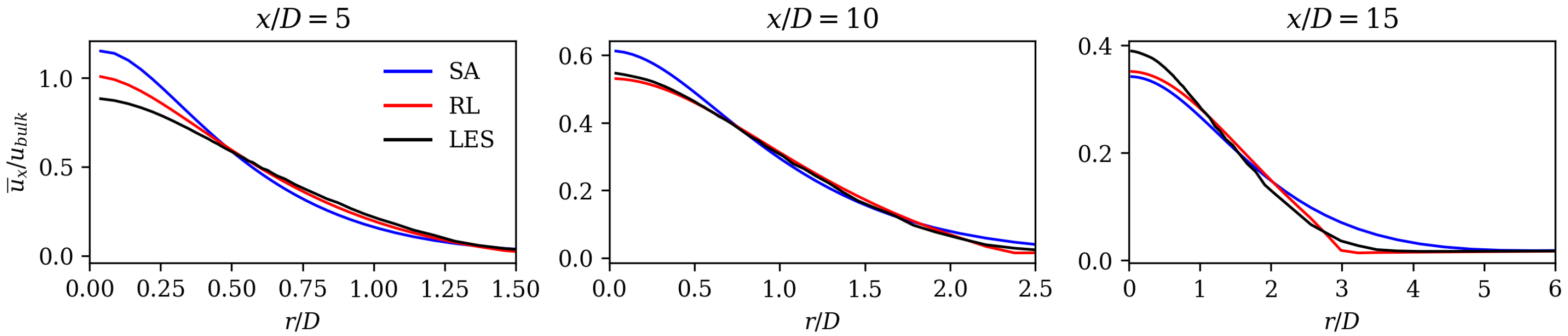
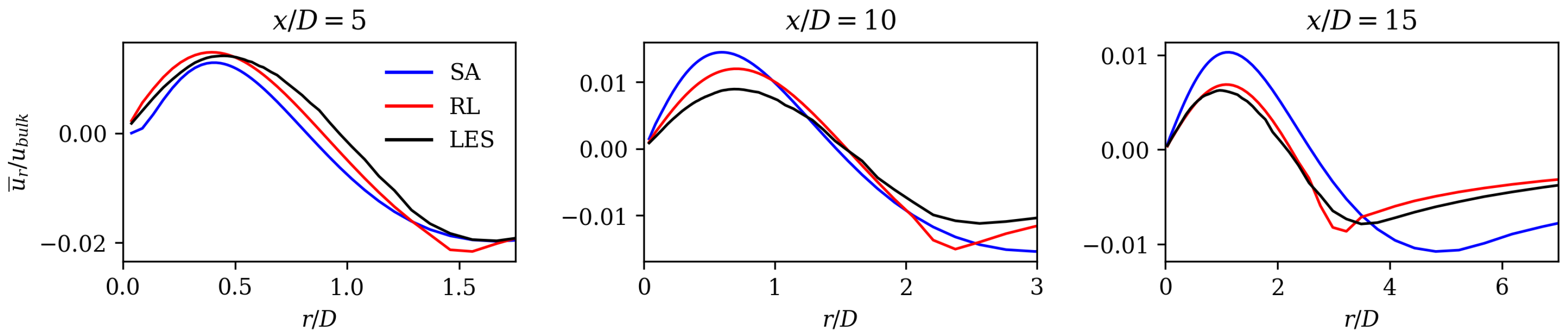
Initially, the velocities were compared because they are decisive for error calculation. Figure 5 and Figure 6 show the axial and radial mean field velocities normed with the bulk velocity at different axial positions (from left to right) of the reference LES data (black line), the SA model (blue line), and RL model results (red line). Overall, it can be observed that the velocity profiles of the RL model are closer to the LES mean fields compared to those of the SA model. The RL model gives better results close to the jet centerline for the axial velocity at and 10, as well as for the radial velocities at and 15.
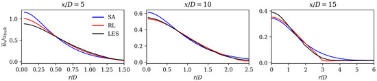
Figure 5.
Normed axial velocity at three different axial positions of SA model, RL model, and LES reference data.
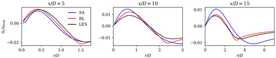
Figure 6.
Normed radial velocity at three different axial positions of SA model, RL model, and LES reference data.
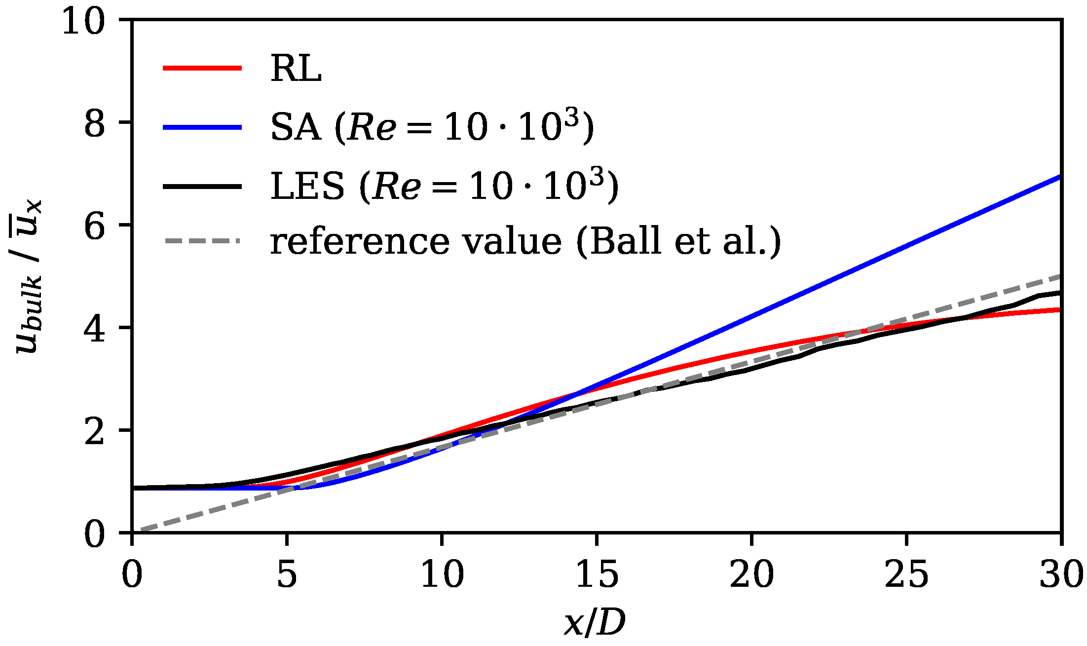
As another measure to assess the augmented Spalart–Allmaras model, the characteristic length and velocity scales of the jet are analyzed. More specifically, we considered the centerline velocity decay and the spreading rate. In previous studies, these quantities have been used to compare experiments with numerical simulations and serve as a good metric for the quality of the turbulence model [61,62,63]. The centerline velocity decay is defined as [64]
where the constant B is the decay rate that depends on the nozzle geometry, is the virtual origin, which is set to , and D is the outlet diameter. According to Ball et al. [64], a decay rate of is observed in the far field of a jet that exits from a converging round nozzle.
Figure 7 shows the axial velocity decay at the jet centerline of the standard SA model, the RL model, and the LES mean field data, and the decay corresponding to . From , all curves reveal a linear trend, as typical for the mean velocity decay. The LES and the RL model results are close to the value of the literature. The SA model shows an increasing discrepancy at . Here, the mean decay rate for the SA model is too pronounced, indicating that the production of turbulence is overpredicted by the standard SA model.
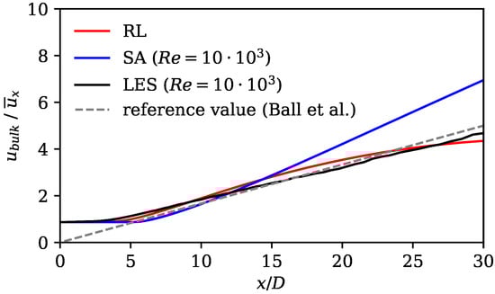
Figure 7.
Axial velocity decay (Equation (9)) showing results of standard SA model, RL model, and LES data, as well as reference value according to Ball et al. [64].
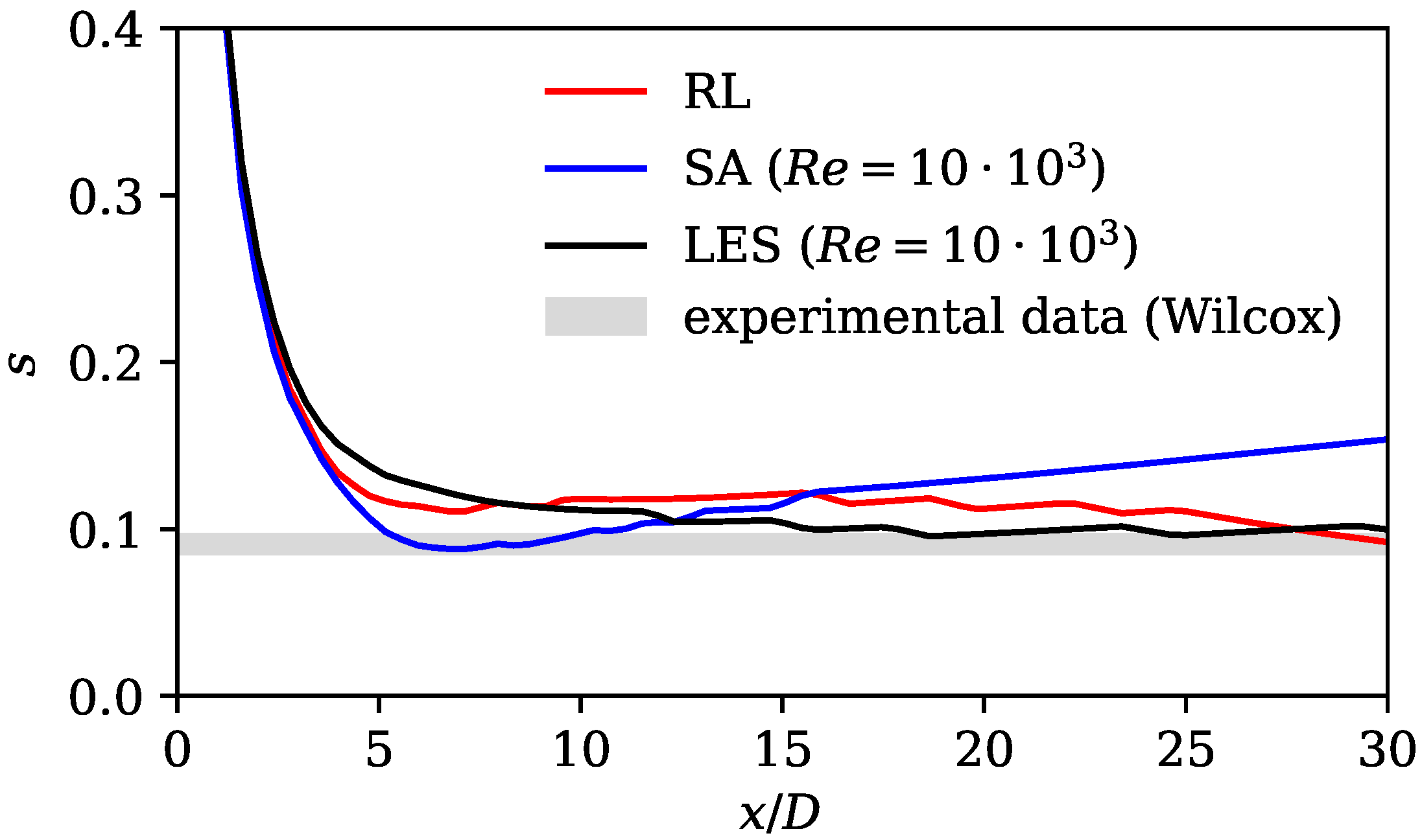
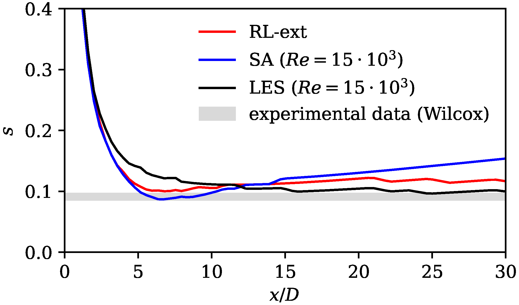
The second characteristic length and velocity scale considered is the spreading rate. It is defined as
where describes the radial position where the axial velocity equals half of the centerline velocity . According to experimental data, the spreading rate is between and in the far field [4]. Figure 8 shows the jet spreading rate for the three cases considered, together with the experimental data according to Wilcox [4]. All curves show large deviations from the literature upstream of . This is expected, as the experimental value only holds in the self-similar far field region of the jet. Apart from a small region near the nozzle between and , where the SA model shows the best prediction of the spreading rate, significant differences between the experimental results and the results based on the standard SA model can be seen. Further downstream and in the majority of the domain, the results of the LES and RL model are very close to the experimental data and show an almost constant spreading rate over a large distance in the direction of flow. In this range, the RL model shows a significant improvement compared to the standard SA model. This shows, again, that the SA model substantially overestimates the turbulent production in the downstream region.

Figure 8.
Spreading rate (Equation (10)) for standard SA model, LES reference mean field data, and RL model. Experimental data and spreading rate definition according to (Wilcox [4] Table 4.1).
To examine the mechanism behind the ability of the RL model to generate more precise spreading rates and mean velocity decay, we examined the eddy viscosity source field. Figure 9f shows the optimal field determined by the DRL algorithm. The RL model adds eddy viscosity in the duct and in the center of the jet, up to an axial coordinate of approximately . In all other regions, there are negative eddy viscosity source values. It should be noted that the inlet boundary conditions for were selected based on standard best practice recommendations [52] without taking additional domain knowledge into account. Apparently, the high source term values in the inlet region compensate for these uncertainties in the initial boundary conditions.

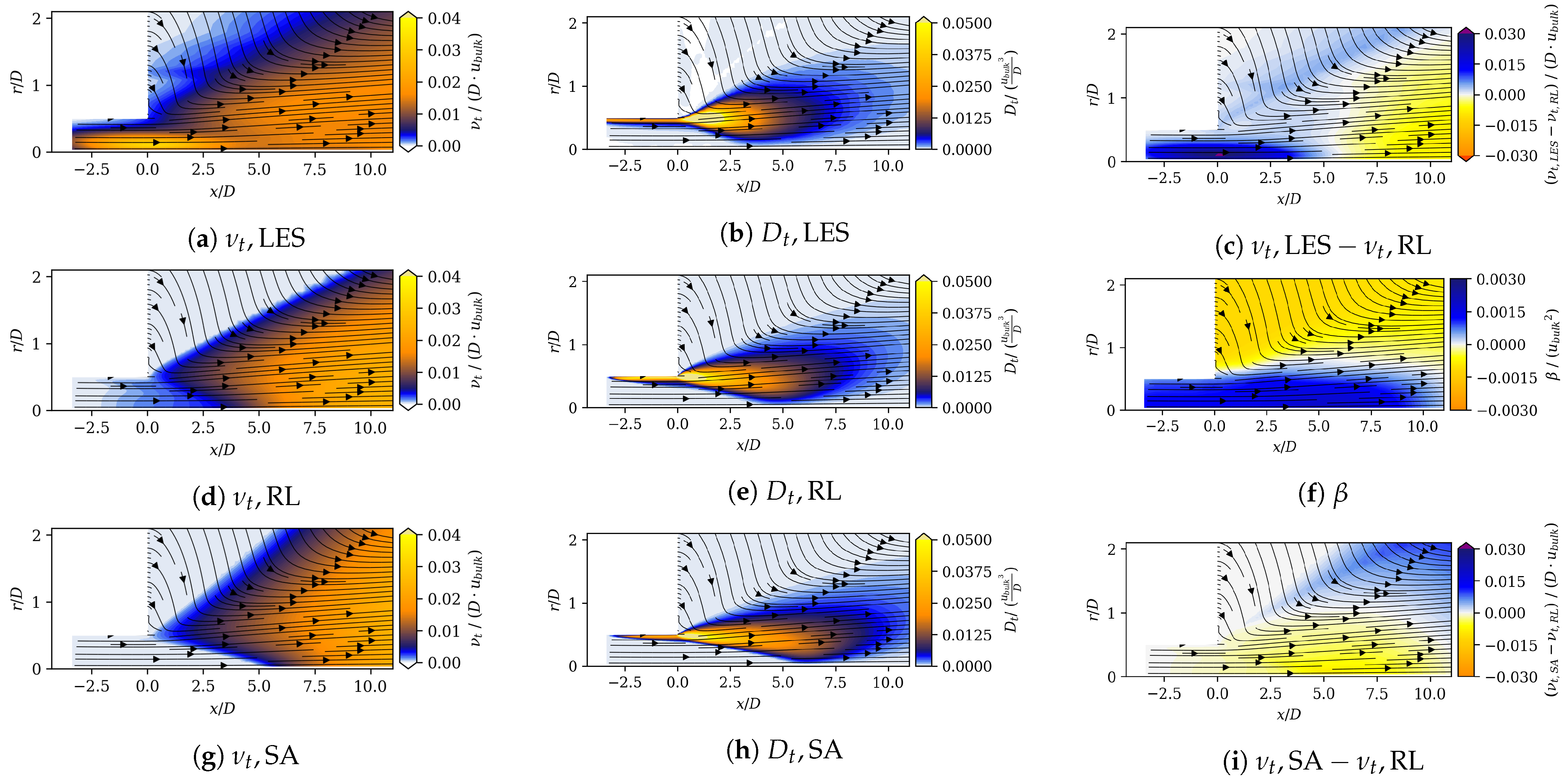
Figure 9.
The left column shows the values of the LES (a), the RL model (d), and the standard SA model (g). The values are non-dimensionalized using the duct diameter D and the bulk velocity . The second column shows the mean field dissipation of the LES (b), the RL model (e), and the standard SA model (h). The values are non-dimensionalized using . Figure (c) shows the difference of the eddy viscosity fields of the LES and the RL model (non-dimensionalized using the duct diameter D and the bulk velocity ). Figure (f) shows the field of the RL model (non-dimensionalized by ). Figure (i) shows the difference of the eddy viscosity fields of the SA model and the RL model (non-dimensionalized using the duct diameter D and the bulk velocity ).
Figure 9d shows the field we obtained from the augmented SA model using the source term . The eddy viscosity field of the unmodified SA model is depicted in Figure 9g. The shape of the fields exhibits qualitatively similar characteristics but quantitatively large discrepancies. The difference in eddy viscosity fields, , is depicted in Figure 9i. The figure illustrates that the RL model has higher values only in the vicinity of the jet centerline behind the duct outlet at 0 to . Downstream and further in the outer regions of the jet, values of the RL model are lower than those of the SA model. On average, the RL model applies smaller -values across the domain.
To validate the eddy viscosities obtained from the (augmented) SA models, we compared them with those estimated from the LES by performing a Boussinesq inversion. This is done by formulating the Boussinesq hypothesis (see Equation (4.45) in Ref. [65]) and applying the boundary layer assumption, reading
which can be solved for based on the LES data. Figure 9a show this quantity, revealing that the LES predicts mainly lower values than the SA and RL model. In the nozzle, however, the values are much higher, revealing substantial turbulent production in the nozzle that is not picked up by the SA and RL models. Overall, the comparison reveals that both the SA and RL models are capable of predicting the eddy viscosity fields reasonably well, catching the right magnitude in the jet core region while showing substantial deviations in the jet boundary.
Next, we considered the mean filed dissipation , which is equivalent to the turbulent production in the RANS framework. This term quantifies the energy transported from the mean to the turbulent field and has a key impact on the mean field solution. The mean field dissipation was determined from the mean energy equations, which was a consequence of contracting the RANS equations with the velocity vector (see Equations (5.135) and (5.143) in Ref. [65]). It reads
which was simplified by employing the boundary layer approximation. This scalar quantity can be compared to the turbulent production (which acts as a dissipation for the mean field) determined from the LES according to
where, again, the boundary layer flow approximation was applied (Equation (5.145) in Ref. [65]). By inspecting these two quantities, we could identify flow regions of high turbulent production and analyze how well this was predicted by the SA- and RL-based eddy viscosity field.
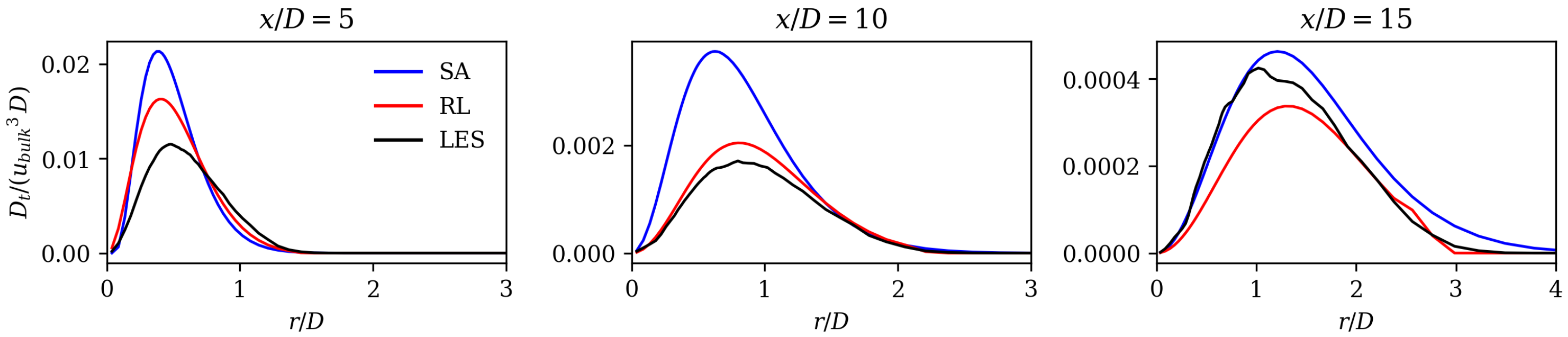
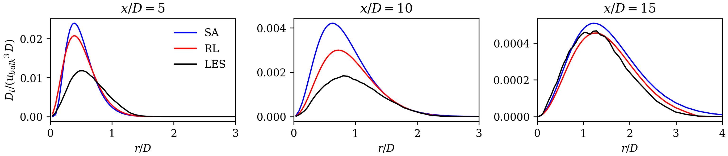
Figure 9b,e,h, display the turbulent production for the LES, and the mean field dissipation predicted by the RL and the SA models, respectively. All three fields show a very similar shape with high values close to the nozzle in a flow region of strong mean shear. To further highlight the differences between the models, Figure 10 shows radial profiles of the same quantities at four axial positions. The presented results show that the SA model overestimates the mean field dissipation (or turbulent production) at 5 and 10, while the RL model shows substantial improvement in that region. Further downstream at 15, the RL model does not show a superior performance compared to the SA model. This is in contrast with the superior prediction of the spreading rates and axial velocity decay values as seen in Figure 7 and Figure 8, which can be attributed to two possible explanations. Firstly, the magnitudes of the values downstream 15 are considerably lower compared to 5 and 10. Secondly, the convection of turbulent kinetic energy may lead to nonlocal effects. In the upstream region at 5 and 10, the RL model demonstrates improved performance compared to the SA model. As turbulence is convected downstream, the local impact of the RL model significantly influences the downstream mean field, even if the values there are not substantially superior to those of the SA model.
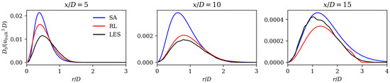
Figure 10.
Non-dimensionalized mean field dissipation at four axial locations for SA model, RL model, and LES.
Overall, Figure 10 clearly shows that the SA model overestimates mean field dissipation and associated turbulent production. This explains why the SA model shows a larger axial velocity decay and a larger spreading rate, because both quantities are affected by a larger energy transfer from the mean to the turbulent field.
3.2. Model Extrapolation to Re = 15,000
To date, we have only considered the results of the model for the case for which the model was also trained. However, one key advantage of DRL, in combination with normalization and the stencil method, is the applicability of trained models to other cases. Since we trained on a jet flow, different geometries are not yet possible. Therefore, we varied the Reynolds number. The extent to which the model is able to extrapolate to a flow with the same geometry at a 50% higher Reynolds number is investigated below.
First, the standard SA model was run at to retrieve the initial state and the reference error . The data’s initial state was decomposed from the stencil approach into several stencil vectors. As the agent’s input data were normalized and non-dimensionalized using the domain’s maximum values, the data required no further treatment. The agent determined the scalar eddy viscosity source values for each cell. The complete field was then used to run a RANS simulation. This process was equal to the framework design, illustrated in Figure 4, without passing the reward to the agent to train it. In this setup, the algorithm was solely used for execution, and its neural network parameters remained unchanged.
Running the case using the standard SA model resulted in a reference error of . With the augmented SA model that uses the -field determined by the extrapolating RL algorithm, an error of was achieved. This corresponds to a relative error reduction of (see Equation (8)).
Figure 11 and Figure 12 show that, for the case, the standard SA model shows a similar deviation from the experiments and LES as for the lower Re case. The jet spreading rate is predicted to be too low and the axial velocity decay too high. The extrapolated RL model counteracts these discrepancies and gives a much better match in both spreading rate and axial velocity decay. Analogously to the lower Reynolds number case, the better match is achieved by an improved prediction of the mean field dissipation using the RL-based model, as shown in Figure 13. When comparing Figure 10 and Figure 13, it is apparent that both the RL model and extrapolating RL model exhibit a similar qualitative improvement in mean field dissipation within the upstream region. However, quantitatively, the improvement over the SA model is less pronounced when the RL model extrapolates.
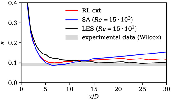
Figure 11.
Spreading rate s for standard SA model and LES reference mean field data for the case and the extrapolating RL model. The extrapolating model was trained on data. Experimental data and spreading rate definition according to (Wilcox [4] Table 4.1).
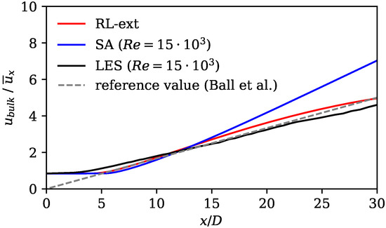
Figure 12.
Axial velocity decay showing results of standard SA model (at ), the extrapolating RL model (trained at ), LES reference data (at ), as well as expected axial mean velocity decay (see Equation (9) and Ref. [64]).
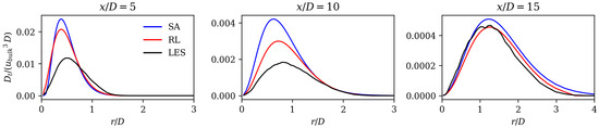
Figure 13.
Non-dimensionalized mean field dissipation at three axial locations for SA model (at ), extrapolating RL model (trained at ), and LES (at ).
To further investigate the generalization performance of the model, we examined the sensitivity to stencil vector changes. The field of the training run and the field of the extrapolating agent exhibited differences of up to . Despite the Reynolds number being 50% larger in the extrapolation case, the stencil vectors differed only by approximately due to the normalization process. This observation suggests that the sensitivity of the algorithm is reasonable. If the observed variation in stencil vector values were to result in either infinitesimally small or excessively large changes in values, it would indicate either a flawed algorithm design or bad generalization performance. However, the fact that such changes in stencil vector values did not lead to extreme deviations in values supports the notion that the algorithm has good generalization performance.
The extrapolation experiment demonstrates the trained agent’s ability to extrapolate to a flow at a higher Reynolds number; however, this is accompanied by a loss of performance. Figure 11, Figure 12 and Figure 13 provide evidence that the solution of the extrapolation exhibits a closer alignment with both the reference data and the expected outcomes described in the literature when compared to the standard SA solution. However, the relative error reduction of the extrapolation case was lower compared to the training case (, ).
4. Discussion
In the following paragraphs, we compare the augmented Spalart–Allmaras model against jet flow-specific closure models, which are tailored for improved accuracy through physics-based reasoning. Subsequently, we compare it with other data-driven methods applied to jet flows. We also highlight the similarities of our methodology with other publications, followed by a discussion of its strengths and limitations.
Ishiko et al. [66] added terms to the Spalart–Allmaras and Menter SST turbulence models to improve the accuracy of free-jet and wall-jet flows. They achieved an improvement in axial velocity decay similar to that of the RL model. Georgiadis et al. [67] compare the performance of turbulence models that were specifically designed for jet flows with standard two-equation models. They also observed delayed axial velocity decay for standard models. The RL model compensates for this disadvantage, as it shows an earlier axial velocity decay (see Figure 7). Its match in axial velocity is comparable to the turbulence models that were designed for jet flows (see Ref. [67]).
He et al. [68] present an adjoint-based data assimilation model that determines a spatially varying correction that is multiplied by the production term of the Spalart–Allmaras governing equation. The eddy viscosity field of the RL model and of the adjoint-based data assimilation model show similar shapes: close to the duct outlet, the eddy viscosity increases, and further downstream, it decreases compared to the SA model [68]. Compared with the results of this work, the approach by He et al. [68] gives a better match in velocities. One fundamental difference is that their model receives reference field data explicitly, as it is implanted in the adjoint-based data assimilation model. In this work, the RL algorithm is not aware of the reference data field directly. It receives a global error that is based on the difference of the velocity fields. The performance of the method can be further improved by increasing the degree of freedom for optimization. He et al. [69] use the adjoint-based data assimilation model to optimize an anisotropic Reynolds stress forcing and exceed the performance of He et al. [68]. In conclusion, both of the data-driven methods discussed that were applied to jet flows [68,69] demonstrate superior performance in matching the reference velocity field compared to the RL model introduced in this work. However, it should be noted that they incorporate greater knowledge of the reference field [68] and have greater degrees of freedom [69].
Despite the success of the current framework, it has two disadvantages: high sensitivity to hyperparameters and high computational costs of performing extensive hyperparameter searches: Small changes in hyperparameter values, simulation setup, or other components of the framework caused substantial performance losses. Conducting extensive hyperparameter searches can quickly become infeasible, due to the high computational costs of training. To get a usable and realistic response (velocity fields) to the agent’s action ( field), the OpenFOAM environment needs to be run for a sufficient number of iterations. For this work, about 50 different hyperparameter configurations were tested to find the best performing model.
One aspect that is known to improve both training speed as well as overall model performance is efficiently leveraging invariants, as highlighted in [23] and demonstrated in [70]. This could be taken into account in future work.
The extrapolation experiment shows that the model is able to extrapolate to a flow with a higher Reynolds number when it is trained on the same geometry. Future studies should investigate whether the model can gain additional robustness by training on two Reynolds numbers in one training run [37]. However, full extrapolation capabilities of the method can only be tested on other flow configurations.
The challenges faced in this work appear to be commonly experienced by others who apply DRL to fluid mechanical problems; Garnier et al. [32] list computational cost and robustness as one of the major challenges other researchers faced. Besides these disadvantages, the proposed method not only generates a solution, but also identifies a model that has the potential to be applied in other cases. An additional advantage of the proposed method is its inherent numerical stability, which stems from its integration of OpenFOAM. Throughout the training process, the algorithm is not rewarded for generating fields that lead to diverging simulations. This ensures that the results obtained from the method maintain numerical stability.
5. Conclusions
In the present study, deep reinforcement learning (DRL) for closure model improvement is investigated. The introduced DRL algorithm searches for an optimal closure field and simultaneously relates it to flow variables by constructing a function that maps the flow field in a surrounding region to a local eddy viscosity source term. This term is directly incorporated into the Spalart–Allmaras turbulence model. The framework is trained and applied to a jet flow configuration at Re = 10,000. Mean fields of high-fidelity LES data are used as reference data. The augmented SA model is applied to a simplified RANS simulation of the reference domain.
The results show substantially improved alignment with the LES reference data and the literature on jet flows. This is shown by analyzing velocity profiles, spreading rates, axial velocity decay rates, and mean field dissipation rates. The error calculated by subtracting the norm of the RANS velocity field and the LES mean fields is improved by the framework by 48%. Moreover, we observe that the RL model counteracts the well-known shortcomings of the SA model without applying physics-based reasoning. The performance of the RL model in the investigated flow region is comparable to that of the models that were tailored for jet flows. In the extrapolation experiment, the model is trained on the Re data and then applied to the Re = 15,000 case. Here, an error reduction of 35% is achieved, proving that the framework is capable of extrapolating to moderately changed flow regimes.
The biggest challenge of this framework is its sensitivity to hyperparameters. Small changes in the hyperparameter values caused substantial changes in model performance. Finding feasible hyperparameter search procedures and identifying critical hyperparameters will remain a big challenge for future applications of reinforcement learning closure models.
Investigating a round jet flow serves as an initial platform to explore the capabilities of the DRL framework. In future studies, more complex flow configurations, including separated flows, are required to fully assess the applicability of DRL for closure modeling.
The introduced reinforcement learning stencil framework successfully identifies a model that has predictive capabilities when applied to the same configuration at a higher Reynolds number, while ensuring numerical stability because it uses OpenFOAM as an interface. The success is encouraging to test the extrapolation capabilities of the method to other geometries and configurations in future studies.
In conclusion, despite facing challenges, this study confirms that deep reinforcement learning represents a promising and novel approach to data-driven closure modeling, which is worth investigating further in more complex configurations.
Author Contributions
Conceptualization, L.M.F., J.G.R.v.S., K.O., and T.L.K.; methodology, L.M.F., J.G.R.v.S., K.O., and T.L.K.; software, L.M.F.; validation, L.M.F., J.G.R.v.S., and K.O.; formal analysis, L.M.F.; investigation, L.M.F.; resources, K.O. and T.L.K.; data curation, T.L.K.; writing—original draft preparation, L.M.F. and J.G.R.v.S.; writing—review and editing, J.G.R.v.S. and K.O.; visualization, L.M.F.; supervision, J.G.R.v.S., K.O., and T.L.K.; project administration, K.O. All authors have read and agreed to the published version of the manuscript.
Funding
Funded by the Deutsche Forschungsgemeinschaft (DFG, German Research Foundation)—504349109, 506170981, 441269395. We acknowledge support by the Open Access Publication Fund of TU Berlin.
Data Availability Statement
The code is openly available at https://github.com/LuFoxDev/DeepRL-augmented-Spalart-Allmaras (accessed on 7 February 2024). The LES mean field data will be made available by the authors on request.
Acknowledgments
The authors would like to express their gratitude towards Feichi Zhang, Thorsten Zirwes and Henning Bockhorn for providing the LES data.
Conflicts of Interest
The authors declare no conflicts of interest.
Abbreviations
The following abbreviations are used in this manuscript:
| CFD | Computational Fluid Dynamics |
| DNS | Direct Numerical Simulation |
| DRL | Deep Reinforcement Learning |
| LES | Large Eddy Simulation |
| PIV | Particle Image Velocimetry |
| RANS | Reynolds Averaged Navier–Stokes Equations |
| RL | Reinforcement Learning |
| SA | Spalart–Allmaras |
| SIMPLE | Semi-Implicit Method for Pressure Linked Equations |
References
- Boussinesq, J. Essai sur la Théorie des Eaux Courantes; Imprimerie Nationale: Paris, France, 1877. [Google Scholar]
- Glegg, S.; Devenport, W. Chapter 8—Turbulence and stochastic processes. In Aeroacoustics of Low Mach Number Flows; Glegg, S., Devenport, W., Eds.; Academic Press: Cambridge, MA, USA, 2017; pp. 163–184. [Google Scholar] [CrossRef]
- Spalart, P.; Allmaras, S. A One-Equation Turbulence Model for Aerodynamic Flows; AIAA: Reston, VA, USA, 1992; p. 439. [Google Scholar] [CrossRef]
- Wilcox, D.C. Turbulence Modeling for CFD, 3rd ed.; DCW Industries: La Canada, CA, USA, 2006. [Google Scholar]
- Menter, F.R. Two-equation eddy-viscosity turbulence models for engineering applications. AIAA J. 1994, 32, 1598–1605. [Google Scholar] [CrossRef]
- Menter, F.R.; Kuntz, M.; Langtry, R. Ten years of industrial experience with the SST turbulence model. Turbul. Heat Mass Transf. 2003, 4, 625–632. [Google Scholar]
- Raje, P.; Sinha, K. Anisotropic SST turbulence model for shock-boundary layer interaction. Comput. Fluids 2021, 228, 105072. [Google Scholar] [CrossRef]
- Menter, F.R.; Matyushenko, A.; Lechner, R. Development of a Generalized K-ω Two-Equation Turbulence Model. In Proceedings of the New Results in Numerical and Experimental Fluid Mechanics XII; Dillmann, A., Heller, G., Krämer, E., Wagner, C., Tropea, C., Jakirlić, S., Eds.; Springer: Cham, Switzeland, 2020; pp. 101–109. [Google Scholar]
- Taghizadeh, S.; Witherden, F.D.; Girimaji, S.S. Turbulence closure modeling with data-driven techniques: Physical compatibility and consistency considerations. New J. Phys. 2020, 22, 093023. [Google Scholar] [CrossRef]
- Foures, D.P.G.; Dovetta, N.; Sipp, D.; Schmid, P.J. A data-assimilation method for Reynolds-averaged Navier–Stokes-driven mean flow reconstruction. J. Fluid Mech. 2014, 759, 404–431. [Google Scholar] [CrossRef]
- Symon, S.; Dovetta, N.; McKeon, B.J.; Sipp, D.; Schmid, P.J. Data assimilation of mean velocity from 2D PIV measurements of flow over an idealized airfoil. Exp. Fluids 2017, 58, 61. [Google Scholar] [CrossRef]
- Franceschini, L.; Sipp, D.; Marquet, O. Mean-flow data assimilation based on minimal correction of turbulence models: Application to turbulent high Reynolds number backward-facing step. Phys. Rev. Fluids 2020, 5, 94603. [Google Scholar] [CrossRef]
- Parish, E.; Duraisamy, K. Quantification of Turbulence Modeling Uncertainties Using Full Field Inversion. In Proceedings of the 22nd AIAA Computational Fluid Dynamics Conference, Dallas, TX, USA, 22–26 June 2015; AIAA: Reston, VA, USA, 2015. [Google Scholar] [CrossRef]
- Singh, A.P.; Duraisamy, K. Using field inversion to quantify functional errors in turbulence closures. Phys. Fluids 2016, 28, 45110. [Google Scholar] [CrossRef]
- von Saldern, J.G.R.; Reumschüssel, J.M.; Kaiser, T.L.; Sieber, M.; Oberleithner, K. Mean flow data assimilation based on physics-informed neural networks. Phys. Fluids 2022, 34, 115129. [Google Scholar] [CrossRef]
- Sliwinski, L.; Rigas, G. Mean flow reconstruction of unsteady flows using physics-informed neural networks. Data-Centric Eng. 2023, 4, e4. [Google Scholar] [CrossRef]
- Volpiani, P.S.; Meyer, M.; Franceschini, L.; Dandois, J.; Renac, F.; Martin, E.; Marquet, O.; Sipp, D. Machine learning-augmented turbulence modeling for RANS simulations of massively separated flows. Phys. Rev. Fluids 2021, 6, 64607. [Google Scholar] [CrossRef]
- Parish, E.J.; Duraisamy, K. A paradigm for data-driven predictive modeling using field inversion and machine learning. J. Comput. Phys. 2016, 305, 758–774. [Google Scholar] [CrossRef]
- Duraisamy, K.; Iaccarino, G.; Xiao, H. Turbulence modeling in the age of data. Annu. Rev. Fluid Mech. 2019, 51, 357–377. [Google Scholar] [CrossRef]
- Xu, R.; Zhou, X.H.; Han, J.; Dwight, R.P.; Xiao, H. A PDE-free, neural network-based eddy viscosity model coupled with RANS equations. Int. J. Heat Fluid Flow 2022, 98, 109051. [Google Scholar] [CrossRef]
- Zhou, X.H.; Han, J.; Xiao, H. Frame-independent vector-cloud neural network for nonlocal constitutive modeling on arbitrary grids. Comput. Methods Appl. Mech. Eng. 2022, 388, 114211. [Google Scholar] [CrossRef]
- Beck, A.; Kurz, M. A perspective on machine learning methods in turbulence modeling. GAMM Mitteilungen 2021, 44, e202100002. [Google Scholar] [CrossRef]
- Kurz, M.; Offenhäuser, P.; Beck, A. Deep reinforcement learning for turbulence modeling in large eddy simulations. Int. J. Heat Fluid Flow 2023, 99, 109094. [Google Scholar] [CrossRef]
- Novati, G.; de Laroussilhe, H.L.; Koumoutsakos, P. Automating turbulence modelling by multi-agent reinforcement learning. Nat. Mach. Intell. 2021, 3, 87–96. [Google Scholar] [CrossRef]
- Silver, D.; Schrittwieser, J.; Simonyan, K.; Antonoglou, I.; Huang, A.; Guez, A.; Hubert, T.; Baker, L.; Lai, M.; Bolton, A.; et al. Mastering the game of go without human knowledge. Nature 2017, 550, 354–359. [Google Scholar] [CrossRef]
- OpenAI. OpenAI Five. 2018. Available online: https://openai.com/research/openai-five (accessed on 7 February 2024).
- Mnih, V.; Kavukcuoglu, K.; Silver, D.; Graves, A.; Antonoglou, I.; Wierstra, D.; Riedmiller, M. Playing Atari with Deep Reinforcement Learning. arXiv 2013, arXiv:1312.5602. [Google Scholar]
- Kober, J.; Bagnell, J.A.; Peters, J. Reinforcement learning in robotics: A survey. Int. J. Robot. Res. 2013, 32, 1238–1274. [Google Scholar] [CrossRef]
- Kiran, B.R.; Sobh, I.; Talpaert, V.; Mannion, P.; Al Sallab, A.A.; Yogamani, S.; Pérez, P. Deep reinforcement learning for autonomous driving: A survey. IEEE Trans. Intell. Transp. Syst. 2021, 23, 4909–4926. [Google Scholar] [CrossRef]
- Uc-Cetina, V.; Navarro-Guerrero, N.; Martin-Gonzalez, A.; Weber, C.; Wermter, S. Survey on reinforcement learning for language processing. Artif. Intell. Rev. 2022, 56, 1543–1575. [Google Scholar] [CrossRef]
- Yu, C.; Liu, J.; Nemati, S.; Yin, G. Reinforcement Learning in Healthcare: A Survey. ACM Comput. Surv. 2021, 55, 1–36. [Google Scholar] [CrossRef]
- Garnier, P.; Viquerat, J.; Rabault, J.; Larcher, A.; Kuhnle, A.; Hachem, E. A review on deep reinforcement learning for fluid mechanics. Comput. Fluids 2021, 225, 104973. [Google Scholar] [CrossRef]
- Larcher, A.; Hachem, E. A review on deep reinforcement learning for fluid mechanics: An update. Phys. Fluids 2022, 34, 111301. [Google Scholar]
- Linot, A.J.; Zeng, K.; Graham, M.D. Turbulence control in plane Couette flow using low-dimensional neural ODE-based models and deep reinforcement learning. Int. J. Heat Fluid Flow 2023, 101, 109139. [Google Scholar] [CrossRef]
- Lee, T.; Kim, J.; Lee, C. Turbulence control for drag reduction through deep reinforcement learning. Phys. Rev. Fluids 2023, 8, 024604. [Google Scholar] [CrossRef]
- Novati, G.; Verma, S.; Alexeev, D.; Rossinelli, D.; Van Rees, W.M.; Koumoutsakos, P. Synchronisation through learning for two self-propelled swimmers. Bioinspir. Biomim. 2017, 12, 036001. [Google Scholar] [CrossRef]
- Tang, H.; Rabault, J.; Kuhnle, A.; Wang, Y.; Wang, T. Robust active flow control over a range of Reynolds numbers using an artificial neural network trained through deep reinforcement learning. Phys. Fluids 2020, 32, 053605. [Google Scholar] [CrossRef]
- Ren, F.; Rabault, J.; Tang, H. Applying deep reinforcement learning to active flow control in weakly turbulent conditions. Phys. Fluids 2021, 33, 037121. [Google Scholar] [CrossRef]
- Rigas, G. Control of Partially Observable Flows with Model-Free Reinforcement Learning. In Proceedings of the APS Division of Fluid Dynamics Meeting Abstracts, Phoenix, AZ, USA, 21–23 November 2021; p. H23-006. [Google Scholar]
- Xia, C.; Zhang, J.; Kerrigan, E.C.; Rigas, G. Active Flow Control for Bluff Body Drag Reduction Using Reinforcement Learning with Partial Measurements. arXiv 2023, arXiv:2307.12650. [Google Scholar] [CrossRef]
- Viquerat, J.; Hachem, E. Parallel Bootstrap-Based On-Policy Deep Reinforcement Learning for Continuous Fluid Flow Control Applications. Fluids 2023, 8, 208. [Google Scholar] [CrossRef]
- Zhu, Y.; Pang, J.H.; Tian, F.B. Stable Schooling Formations Emerge from the Combined Effect of the Active Control and Passive Self-Organization. Fluids 2022, 7, 41. [Google Scholar] [CrossRef]
- Shimomura, S.; Sekimoto, S.; Oyama, A.; Fujii, K.; Nishida, H. Closed-loop flow separation control using the deep q network over airfoil. AIAA J. 2020, 58, 4260–4270. [Google Scholar] [CrossRef]
- Fan, D.; Yang, L.; Wang, Z.; Triantafyllou, M.S.; Karniadakis, G.E. Reinforcement learning for bluff body active flow control in experiments and simulations. Proc. Natl. Acad. Sci. USA 2020, 117, 26091–26098. [Google Scholar] [CrossRef] [PubMed]
- Kim, J.; Kim, H.; Kim, J.; Lee, C. Deep reinforcement learning for large-eddy simulation modeling in wall-bounded turbulence. Phys. Fluids 2022, 34, 105132. [Google Scholar] [CrossRef]
- Yousif, M.Z.; Zhang, M.; Yang, Y.; Zhou, H.; Yu, L.; Lim, H. Physics-guided deep reinforcement learning for flow field denoising. arXiv 2023, arXiv:2302.09559. [Google Scholar]
- Cato, A.S.; Volpiani, P.S.; Mons, V.; Marquet, O.; Sipp, D. Comparison of different data-assimilation approaches to augment RANS turbulence models. Comput. Fluids 2023, 266, 106054. [Google Scholar] [CrossRef]
- Zhang, F.; Zirwes, T.; Habisreuther, P.; Bockhorn, H.; Trimis, D.; Nawroth, H.; Paschereit, C.O. Impact of Combustion Modeling on the Spectral Response of Heat Release in LES. Combust. Sci. Technol. 2019, 191, 1520–1540. [Google Scholar] [CrossRef]
- Casel, M.; Oberleithner, K.; Zhang, F.; Zirwes, T.; Bockhorn, H.; Trimis, D.; Kaiser, T.L. Resolvent-based modelling of coherent structures in a turbulent jet flame using a passive flame approach. Combust. Flame 2022, 236, 111695. [Google Scholar] [CrossRef]
- Baldwin, B.; Barth, T. A One-Equation Turbulence Transport Model for High Reynolds Number Wall-Bounded Flows; AIAA Paper 91-0610; AIAA: Reston, VA, USA, 1991. [Google Scholar]
- OpenFOAM Foundation. Spalart–Allmaras Source Code—OpenFOAM/OpenFOAM-4.x. 2016. Available online: https://github.com/OpenFOAM/OpenFOAM-4.x/blob/master/src/TurbulenceModels/turbulenceModels/RAS/SpalartAllmaras/SpalartAllmaras.H (accessed on 18 September 2023).
- Rumsey, C.; NASA—Langley Research Center—Turbulence Modeling Resource. The Spalart–Allmaras Turbulence Model. 2022. Available online: https://turbmodels.larc.nasa.gov/spalart.html (accessed on 11 September 2023).
- Tracey, B.; Duraisamy, K.; Alonso, J.J. A machine learning strategy to assist turbulence model development. In Proceedings of the 53rd AIAA Aerospace Sciences Meeting, Kissimmee, FL, USA, 5–9 January 2015; pp. 1–23. [Google Scholar] [CrossRef]
- ESI-OpenCFD. 4.3 Mesh Generation with the BlockMesh Utility. 2022. Available online: https://www.openfoam.com/documentation/user-guide/4-mesh-generation-and-conversion/4.3-mesh-generation-with-the-blockmesh-utility (accessed on 18 September 2023).
- Sutton, R.S.; Barto, A.G. Reinforcement Learning: An Introduction, 2nd ed.; The MIT Press: Cambridge, MA, USA, 2020. [Google Scholar]
- Kuhnle, A.; Schaarschmidt, M.; Fricke, K. Tensorforce: A TensorFlow Library for Applied Reinforcement Learning. 2017. Available online: https://tensorforce.readthedocs.io/en/latest/ (accessed on 2 October 2023).
- Schulman, J.; Wolski, F.; Dhariwal, P.; Radford, A.; Klimov, O. Proximal policy optimization algorithms. arXiv 2017, arXiv:1707.06347. [Google Scholar]
- Viquerat, J.; Rabault, J.; Kuhnle, A.; Ghraieb, H.; Larcher, A.; Hachem, E. Direct shape optimization through deep reinforcement learning. J. Comput. Phys. 2021, 428, 110080. [Google Scholar] [CrossRef]
- Ghraieb, H.; Viquerat, J.; Larcher, A.; Meliga, P.; Hachem, E. Single-step deep reinforcement learning for open-loop control of laminar and turbulent flows. Phys. Rev. Fluids 2021, 6, 053902. [Google Scholar] [CrossRef]
- Vinuesa, R.; Lehmkuhl, O.; Lozano-Durán, A.; Rabault, J. Flow Control in Wings and Discovery of Novel Approaches via Deep Reinforcement Learning. Fluids 2022, 7, 62. [Google Scholar] [CrossRef]
- Yoder, D.; DeBonis, J.; Georgiadis, N. Modeling of turbulent free shear flows. Comput. Fluids 2015, 117, 212–232. [Google Scholar] [CrossRef]
- Winant, C.D.; Browand, F.K. Vortex pairing: The mechanism of turbulent mixing-layer growth at moderate Reynolds number. J. Fluid Mech. 1974, 63, 237–255. [Google Scholar] [CrossRef]
- Goebel, S.G.; Dutton, J.C. Experimental study of compressible turbulent mixing layers. AIAA J. 1991, 29, 538–546. [Google Scholar] [CrossRef]
- Ball, C.G.; Fellouah, H.; Pollard, A. The flow field in turbulent round free jets. Prog. Aerosp. Sci. 2012, 50, 1–26. [Google Scholar] [CrossRef]
- Pope, S.B. Turbulent Flows; Cambridge University Press: Cambridge, UK, 2000. [Google Scholar] [CrossRef]
- Ishiko, K.; Hashimoto, A.; Matsuo, Y.; Yoshizawa, A.; Nishiyama, Y.; Mori, K.; Nakamura, Y. One-Equation Extended Nonlinear Turbulence Modeling in Predicting Three-Dimensional Wall Jets. J. Aircr. 2014, 51, 584–595. [Google Scholar] [CrossRef]
- Georgiadis, N.J.; Yoder, D.A.; Engblom, W.A. Evaluation of modified two-equation turbulence models for jet flow predictions. AIAA J. 2006, 44, 3107–3114. [Google Scholar] [CrossRef]
- He, C.; Liu, Y.; Gan, L. A data assimilation model for turbulent flows using continuous adjoint formulation. Phys. Fluids 2018, 30, 105108. [Google Scholar] [CrossRef]
- He, C.; Wang, P.; Liu, Y. Data assimilation for turbulent mean flow and scalar fields with anisotropic formulation. Exp. Fluids 2021, 62, 117. [Google Scholar] [CrossRef]
- Vignon, C.; Rabault, J.; Vasanth, J.; Alcántara-Ávila, F.; Mortensen, M.; Vinuesa, R. Effective control of two-dimensional Rayleigh-Bénard convection: Invariant multi-agent reinforcement learning is all you need. Phys. Fluids 2023, 35, 065146. [Google Scholar] [CrossRef]


Disclaimer/Publisher’s Note: The statements, opinions and data contained in all publications are solely those of the individual author(s) and contributor(s) and not of MDPI and/or the editor(s). MDPI and/or the editor(s) disclaim responsibility for any injury to people or property resulting from any ideas, methods, instructions or products referred to in the content. |
© 2024 by the authors. Licensee MDPI, Basel, Switzerland. This article is an open access article distributed under the terms and conditions of the Creative Commons Attribution (CC BY) license (https://creativecommons.org/licenses/by/4.0/).