Numerical Analysis of Convective Heat Transfer in Quenching Treatments of Boron Steel under Different Configurations of Immersed Water Jets and Its Effects on Microstructure

Abstract

In this work, the effects of jet impact angle and water flow on the heat-transfer coefficient in boron steel probes were analyzed. Angles of 90°, 75° and 60° were used with stirring flows of 33 l·min⁻¹, 25 l·min⁻¹, 13 l·min⁻¹ and 6 l·min⁻¹. The aim consisted of determining the heat-extraction rates by analyzing the correlation programmed in the Ansys Fluent 2020R2 software when different cooling conditions are used, avoiding many experiments, and establishing quenching conditions free of surface defects on the workpiece. This process is currently used in heavy machinery, requiring high hardness and wear resistance. The fluid-dynamic field was validated using a scale physical model using the particle image velocimetry technique, PIV. In contrast, the thermal field was validated with transient state experiments solving the inverse heat conduction problem, IHCP. The results show that for high flows (33 l·min⁻¹), the jets with an angle of 90° impact the entire surface of the piece, but their cooling rate is slower compared to the other angles, being 243.61 K·s⁻¹, and 271.70 K·s⁻¹, 329.56 K·s⁻¹ for 75° and 60°, respectively. However, for low flows (6 l·min⁻¹), the impact velocities are very similar for the three cases, promoting more homogeneous cooling rates of 58.47 K·s⁻¹, 73.58 K·s⁻¹ and 63.98 K s⁻¹ for angles of 90°, 75° and 60°, respectively. Likewise, through the use of CCT diagrams, it was determined that regardless of the cooling rate, the final structure will always be a mixture of martensite–bainite due to the effect of boron as determined experimentally, which implies a more significant proportion of martensite at higher cooling rates.

1. Introduction

Quenching steel parts involves cooling processes under controlled conditions to obtain microstructures and specific mechanical properties. Thus, there are many variables to evaluate the capacity of cooling media under different conditions (with and without agitation). Various investigations have been conducted to evaluate the cooling medium’s effect on fluid dynamics, heat extraction and its effect on phase transformation. Studies [1,2] have been carried out exclusively in fluid dynamics to evaluate the cooling medium’s behavior when confined in a quenching tank. In these investigations, only the continuity equations and the Navier–Stokes equations have been solved in conjunction with the turbulence model; B. Hernández Morales et al. [1] developed a study of the behavior of hydrodynamics in the quenching of flat-end cylindrical probes subjected to a Jominy-type test in order to evaluate the effect of wettability in this type of geometries. Kumar et al. [2] evaluated the uniformity of the flow around pinions for automotive applications during the quenching of this type of parts. Other investigations [3,4,5] have focused on the effects that occur when stirring the fluid through propeller arrangements; Xia-wei Yang et al. [3], with a two-propeller arrangement, determined that increasing the stirring velocity can provide a large flow of water in the cooling zone, but also increases fluctuations in the flow velocity in the zone. D. R. Garwood et al. [4] modeled the distribution of oil flow in an agitated quenching tank using four propellers, which is used for the heat treatment of superalloy forgings, validating their calculations using a physical model where velocities were measured with anemometry laser. Nailu Chen et al. [5] investigated the effect of flow directors in quenching with agitation produced by a propeller to evaluate the uniformity of the velocity and distribution of the flow in the quenching area of the piece and thus obtain a more homogeneous cooling of the pieces. On the other hand, experiments have been carried out under steady-state conditions [6,7]. Halva and Volný [8] calculated the fluid flow to examine the homogeneity of the distribution of velocities as a function of the location of the stirrers. Xia-wei Yang et al. [9] evaluated the velocity and uniformity of the fluid-dynamic field in two types of quenching tanks (with and without agitation); they determined that for the case without agitation, the flow is not regular, while with the model with agitation, the flow fields present areas of better regularity. Currently, there are new contributions where the transient-state energy equation is solved simultaneously using CFD to determine the evolution of the temperature of a solid body within the computational domain [10,11,12]. Gomes et al. [12] developed a mathematical model to predict the temperature profile in a steel pipe and studied the effect of water-flow rate and pressure in the heat treatment. It is well known that the boiling state of liquid cooling is distinguished because the vapor film appearance and the bubbles’ formation are involved, resulting in a complex process to model. Even so, research has been developed to consider the two-phase flow (vapor and liquid) formed during this stage [13,14,15,16,17,18]; however, to take this into account, empirical expressions need to be calculated to solve the rate of mass, momentum, and energy exchange between phases. These contributions have helped other authors ensure that the data obtained from mathematical simulations can be used to further predict the microstructure that can be obtained in the workpieces when subjected to cooling [19]. Wang et al. [20] carried out a finite element model of carburizing and quenching in helical gear made of 20CrMnTiH steel; in this model, the mutual coupling between the phase transformation field, stress–strain field, and temperature field were considered. This coupling effect was based on the metal–thermal–mechanics theory of continuous thermodynamics. Mehran et al. [21] developed a quenching jet impingement process simulation to study the effects of liquid jets on heat transfer, and the phase change was added to the OpenFOAM solver’s code.

This work aims to implement a practical methodology and an integral analysis through numerical and experimental simulation to elucidate the susceptibility of damage (distortion or cracking) during quenching of boron steel parts in a tank with immersed jets, varying the water-flow parameters and incident jet angle on the metal piece.

2. Computational Domain

Figure 1a shows a 3D isometric view of the numerical domain employed to analyze the impact effect of the jet on the pieces subjected to quenching through ANSYS-Fluent 2020R^®. The boundary conditions for this study’s solution of the fluid-dynamic field are also appreciated. On the other hand, Figure 1b,c show front and side views with dimensions of the computational domain, in which the location of the jets and how they impact perpendicularly to the steel probe.

Inlet flows of 33 l·min⁻¹, 25 l·min⁻¹, 13 l·min⁻¹ and 6 l·min⁻¹ were used for each of the angles and jets in the computational domain. The experimental matrix of the studied cases is shown in

Table 1. Experimental matrix of the studied cases.

Case	Angle	Flow, l·min−1
1	90°	33
2		25
3		13
4		6
5	75°	33
6		25
7		13
8		6
9	60°	33
10		25
11		13
12		6

, where case 1 was used to validate the mathematical model.

2.1. Governing Equations

The continuity and momentum equations were solved under turbulent and transient flow conditions to obtain flow patterns in the computational domain generated by the water flowing through each quenching tank jet.

$$\frac{\partial }{\partial t}\rho +\nabla \cdot \left(\rho \overrightarrow{v}\right)=0$$

(1)

$$\rho \left[\frac{\partial \overrightarrow{v}}{\partial t}+\left(\overrightarrow{v}\cdot \nabla \right)\overrightarrow{v}\right]+\nabla p-\nabla \cdot \tau =\rho \overrightarrow{g}$$

(2)

where $\rho$ is the fluid density, kg·m⁻³, $\overrightarrow{v}$ is the fluid velocity, m·s⁻¹, $p$ is the dynamic pressure, Pa, τ is the shear stress due to viscous flow, N·m⁻² and $\overrightarrow{g}$ is the acceleration due to gravity, m·s⁻². The turbulence model implemented is the Realizable k-ε model, which has superior characteristics than the standard model in terms of curvature and rotation in flows with turbulent streams, which solves two equations: one for the turbulent kinetic energy, k, Equation (3), and another for the dissipation of turbulent kinetic energy, ε, Equation (4).

$$\frac{\partial }{\partial t}\left(\rho k\right)+\frac{\partial }{\partial t}\left(\rho k{u}_j\right)=\frac{\partial }{\partial x_j}\left[\left(\mu +\frac{{\mu }_t}{{\sigma }_k}\right)\frac{\partial k}{\partial x_j}\right]+G_k+G_b-\rho \epsilon -Y_M$$

(3)

$$\frac{\partial }{\partial t}\left(\rho \epsilon \right)+\frac{\partial }{\partial x_j}\left(\rho \epsilon u_j\right)=\frac{\partial }{\partial x_j}\left[\left(\mu +\frac{{\mu }_t}{{\sigma }_{\epsilon }}\right)\frac{\partial \epsilon }{\partial x_j}\right]+\rho C_1{S}_{\epsilon }-\rho C_2\frac{{\epsilon }^2}{k+\sqrt{v\epsilon }}+C_{1\epsilon }\frac{\epsilon }{k}{G}_b$$

(4)

where, k is the turbulent kinetic energy, J·kg⁻¹, and ε is the dissipation of turbulent kinetic energy, m²·s⁻³, μ is the dynamic viscosity, kg·m⁻¹·s⁻¹, μ_t is the turbulent dynamic viscosity, m²·s⁻¹, σ_k and σ_ε are the Prandtl number as a function of k and ε with values of 1.0 and 1.2, respectively, Gk and Gb represent the energy generation turbulent kinetics due to velocity and buoyancy gradients, respectively, C₁ε and C₂ are constants with values of 1.44 and 1.9, respectively. The domain was discretized using hexahedral elements for the steel probes and tetrahedral elements for the quenching vessel; a total of 1,345,392 elements were used to carry out the numerical simulation. The coupling of the pressure and velocity fields was solved using the SIMPLEC [22] method.

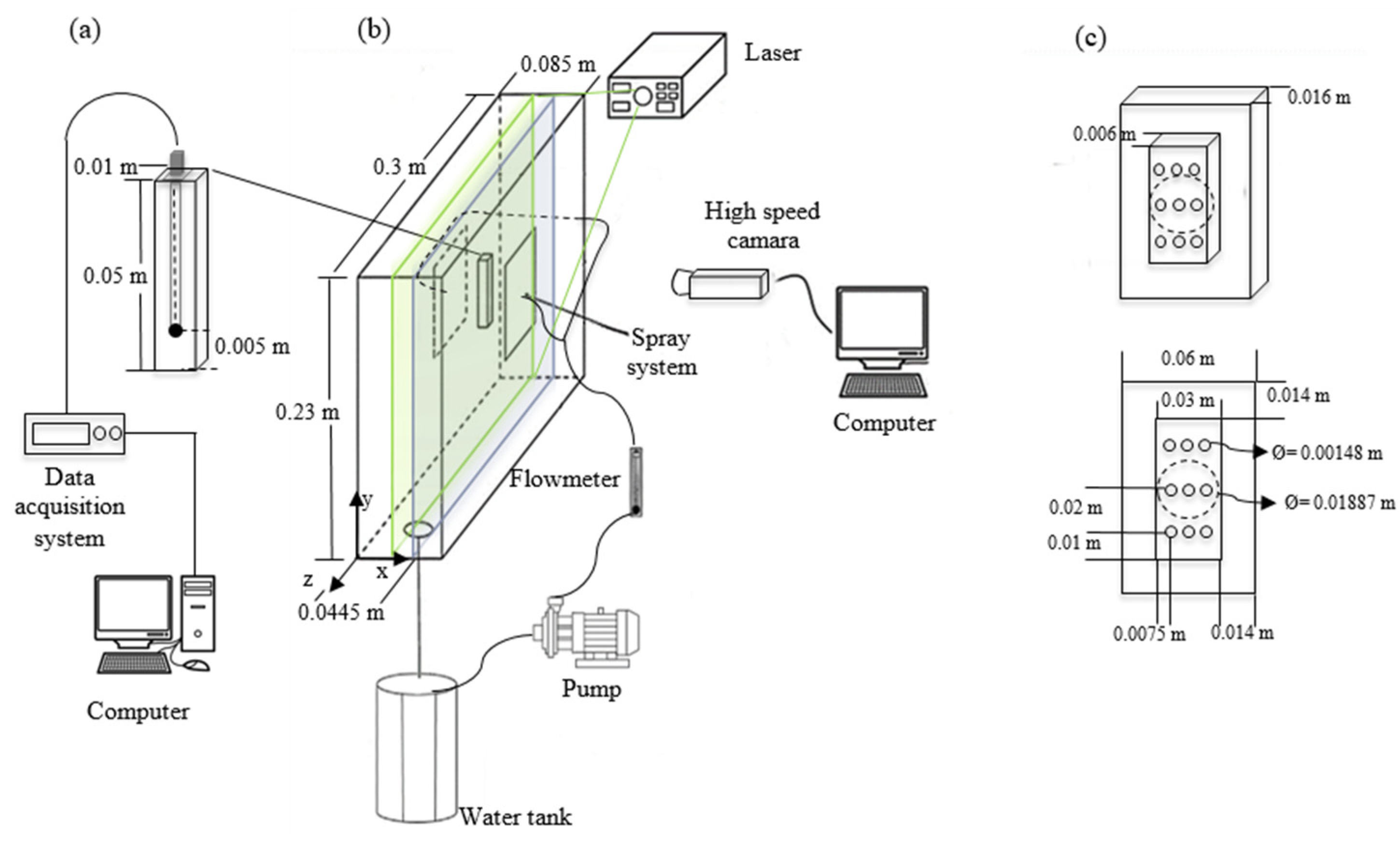
2.2. Physical Modeling Employing PIV and Thermal Histories

Figure 2 illustrates the experimental setup of a 1:6 scale model of the quenching tank with the jets at 90°, used to validate the fluid-dynamic field. This model was made of a 6 mm thick transparent Perspex sheet, and the probe steel was made of square section. For obtaining the flow patterns, PIV technique was employed; Figure 2b shows a representative scheme of the system to experiment, while Figure 2c illustrates in detail the dimensions and geometry of the flow jets system. These jets impact both sides of the vessel, consisting of a chamber with an inlet orifice of 0.01887 m, and divide the water flow into nine jets. The tests were carried out with a flow of 6 l·min⁻¹, and the selected study longitudinal plane was located perpendicular to x-axis at 0.0445 m, as shown in Figure 2b. A 4 HP pump allowed the fluid to pass until the flow meter, which was established at 6 l·min⁻¹, then this flow was divided into two to direct the water to the jet system. Once the desired water level was reached (~0.22 m) in the quenching tank, the flow outlet located at the bottom was regulated by a ¾ in. globe valve, the water level and cooling conditions have already been established proposed operation, the data were obtained to determine the average fluid-dynamic field. To validate the thermal distribution in the numerical model, a square section specimen from AISI-SAE 15B35H steel with dimensions of 0.05 m long and 0.01 m wide was machined and instrumented with a K-type thermocouple introduced at a depth of the base, as shown in Figure 2a [23,24]. The thermocouple signal was recorded by a FLUKE NetDAQ 2645A data acquisition system with a sampling frequency of 60 Hz. The procedure consisted of heating the specimens in a vertical resistance furnace up to the austenitization temperature of ~1143 K, with a holding time of 15 min. Subsequently, the probe was subjected to quenching with a cooling water temperature of 298 K. Once the thermal history was obtained with the experimental system, the heat transfer was calculated by solving the inverse heat conduction problem, IHCP, as previously described [25,26,27]. Equation (5) mathematically describes the problem where r is the radial distance of the probe, m; T is the temperature, K; t is the cooling time, s; k, ρ, and Cp are the thermal conductivity, W·m⁻¹·K⁻¹; density, kg·m⁻³; and the specific heat of the material, in J·kg⁻¹·K⁻¹, respectively.

$$\frac{1}{r}\frac{\partial }{\partial r}\left(kr\frac{\partial T}{\partial t}\right)=\frac{\partial }{\partial t}\left(\rho CpT\right)$$

(5)

For the solution of Equation (5), the following boundary conditions were used:

• There is no heat transfer in the symmetry axis of the specimen, so it is considered an isolated boundary, as shown in Equation (6).

$$\frac{\partial T}{\partial r}=0, at r=0(\mathrm{symmetry})$$

(6)

• The heat that arrives by conduction to the surface in contact with the fluid is transferred to the surroundings by forced convection, represented in Equation (7) by a global heat transfer coefficient h

$$-k\frac{\partial T}{\partial r}=h\left(Tf-T\right),at r=R\left(convection\right)$$

(7)

The surface heat flux density is estimated from the knowledge of the temperature measured inside a heat-conducting solid by minimizing the function of Equation (8).

$$F(q)={\displaystyle \sum _{i=1}^{Ms}{(T_{n+1}-Y_{n+1})}^2}$$

(8)

where M = θ·t⁻¹, for regular finite intervals, θ and t are the time steps to calculate the heat flux and temperature, respectively, T_n and Y_n are the measured temperatures close to the metal-liquid interface, K. This procedure is repeated until a convergence criterion of less than 0.005 is obtained and allows simultaneously obtaining the temperature of the surface of the sample in contact with the cooling medium and the interfacial heat flow. Finally, the heat-transfer coefficients h of the surface in contact with the quenching fluid were calculated through Newton’s cooling law according to Equation (9), where q is the heat flow on the surface at the solid–liquid interface, W·m⁻², T and T_f are the calculated surface temperature and saturation temperature of the fluid, K, respectively.

$$h=\frac{q}{\left(T-Tf\right)}$$

(9)

3. Analysis and Discussion of Results

3.1. Validation

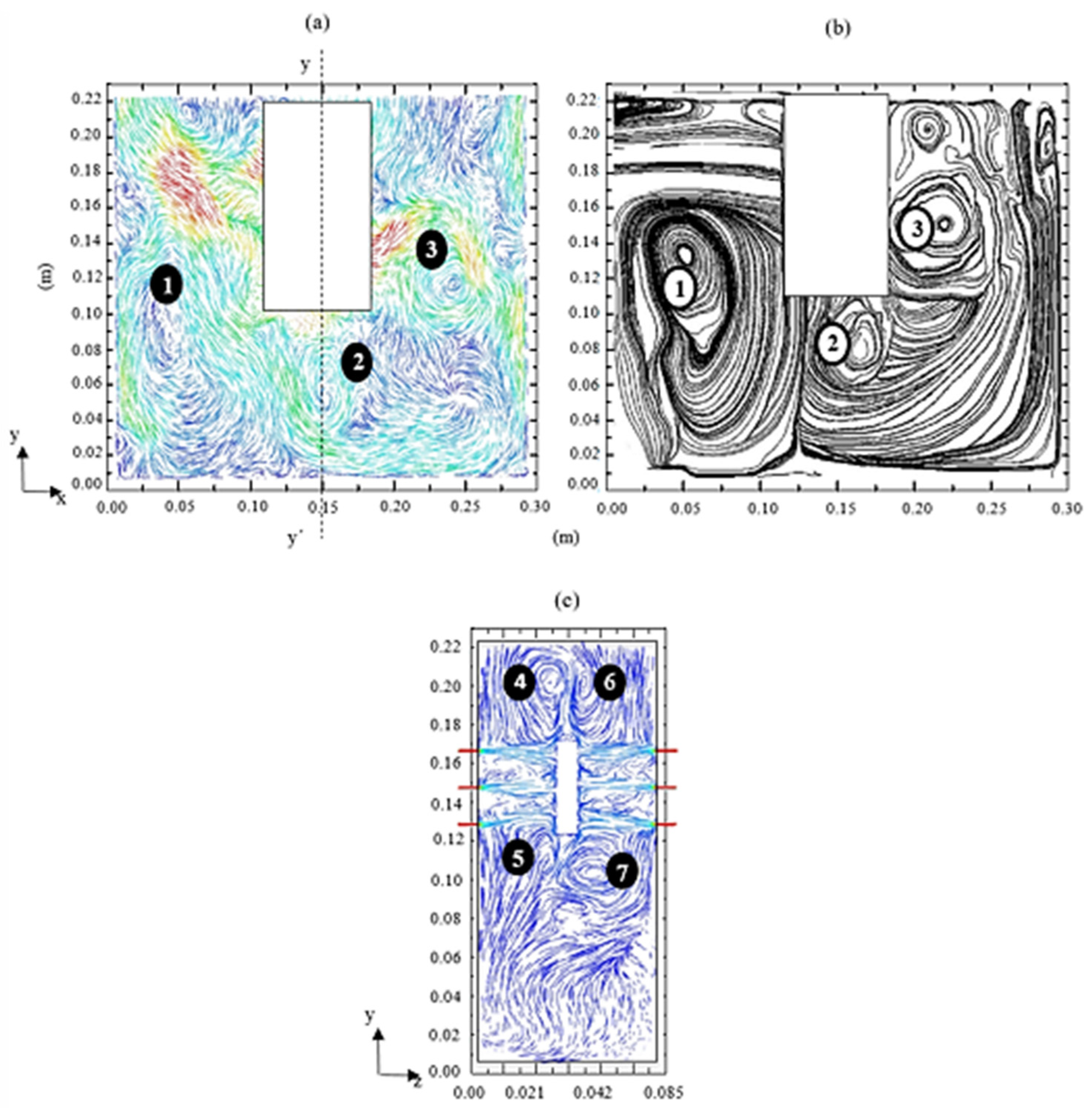
3.1.1. Dynamic Fluid Field

The fluid-dynamic structure inside the quenching tank was obtained by dispersing 20 mm diameter polyamide particles using the PIV technique, where the flow patterns were obtained in the physical model. Figure 3 shows a comparison between both techniques, the experimental model (Figure 3a) and the numerical model (Figure 3b), in which a blank box is observed corresponding to the jet system, where they are impacting perpendicularly to the -xy plane. In both techniques, the formation of three main recirculations is distinguished and agreed; the flow currents define the formation of these recirculations; the recirculation existing on the left border of the quenching tank denoted by points ① and ❶, as well as the one existing on the right side ③ and ❸ and a small recirculation existing in the lower central area ② and ❷. A transverse plane was analyzed in the y-y’ section in which the impact of the jets on the piece can be seen and where the fluid-dynamic structure that is presented is symmetrical since four recirculations are developed: two superiors, ❹ and ❻, and two lower ❺ and ❼, which are formed because the opening angle of the upper and lower jets is broad, in such a way that it generates a compression of the row of jets in the middle section and in turn they disperse in free currents in the upper and lower areas of the vessel, forming such recirculations.

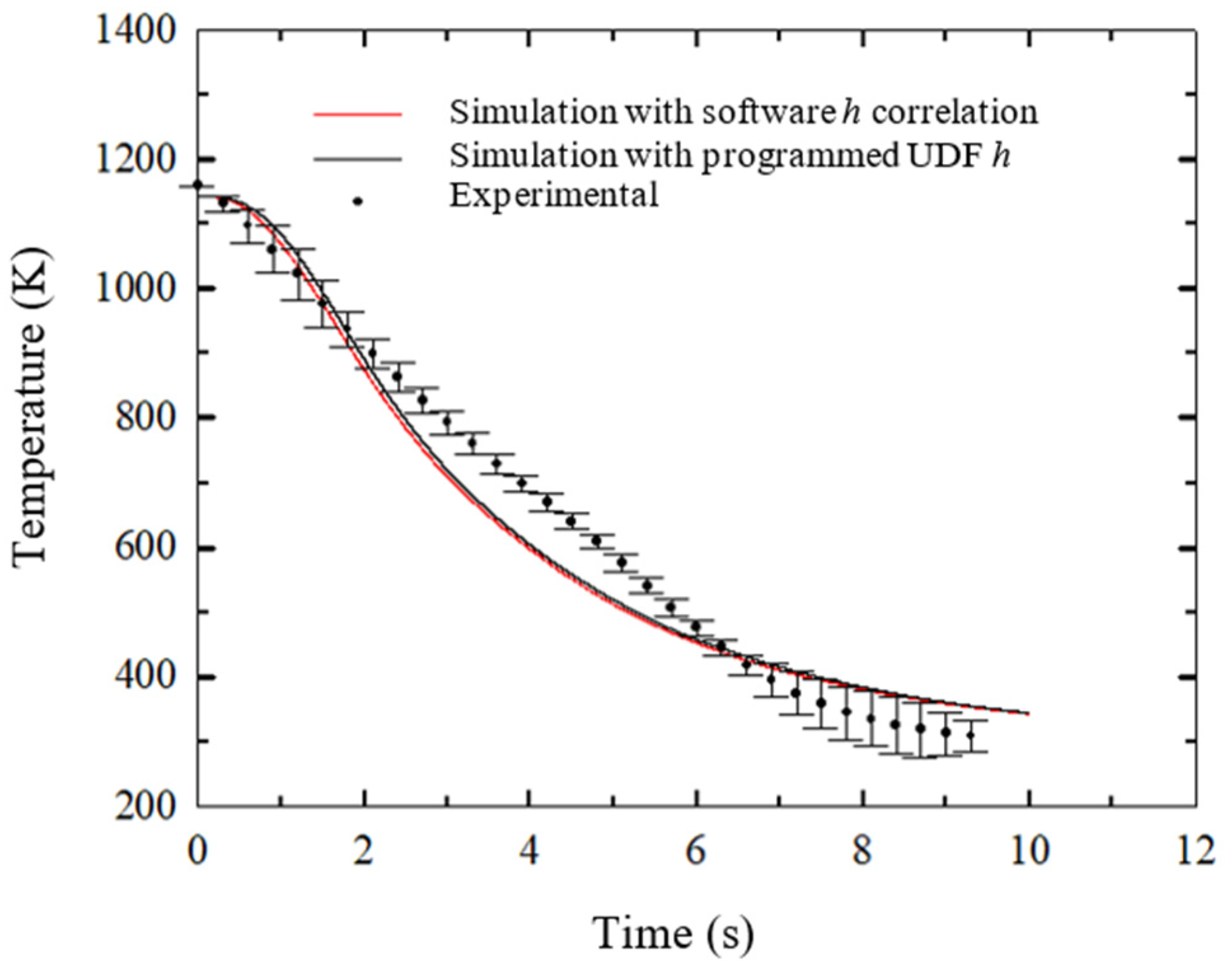
3.1.2. Thermal Field Validation

Figure 4 shows the validation of the thermal field where three cooling curves are compared: one experimental and two correlations used in the numerical simulation; the Equation (10) was obtained by an eight-order polynomial regression of plotted heat-transfer coefficient as a function of time, from the experimental data obtained:

$$\begin{array}{l}h=-0.780132x{t}^8+27.9553x{t}^7-401.918x{t}^6+2999.11x{t}^5-12505.6x{t}^4\\ +29,160.7x{t}^3-35,603.8x{t}^2+19841xt-106.216\end{array}$$

(10)

This correlation was introduced as a user-defined function, UDF, into the solution of the energy equation. The second expression employed, Equation (11), is programmed by default in the software.

$$h=\frac{\rho C_p{C_{\mu }}^{1/4}{k}^{1/2}}{T_{ref}}$$

(11)

where $\rho$ is the density, kg·m⁻³, C_p is the heat capacity, J·kg⁻¹·K⁻¹, C_µ is a constant with a value of 0.009, k is the turbulent kinetic energy, in J·kg⁻¹, and T_ref is a reference temperature, K. The experimental curve was made with three tests conducted under the same conditions to corroborate the experiment’s reproducibility. It can be seen that the other two curves have differences between 2 to 6 s concerning the plotted experimentally; this is due to the formation of the oxide scale released after cooling [28]. For the curves obtained from mathematical simulation, relative errors were calculated concerning the average experimental curve, which was ~8% with the “h” programmed as UDF and ~9.07% for the correlation of “h” by default in the software. These model adjustments produced results closer to each other, and both are within an acceptable range of error [29] since implementing a UDF requires experimental data for each individual case; for the subsequent study cases in Table 1, the correlation of Equation (11) was employed.

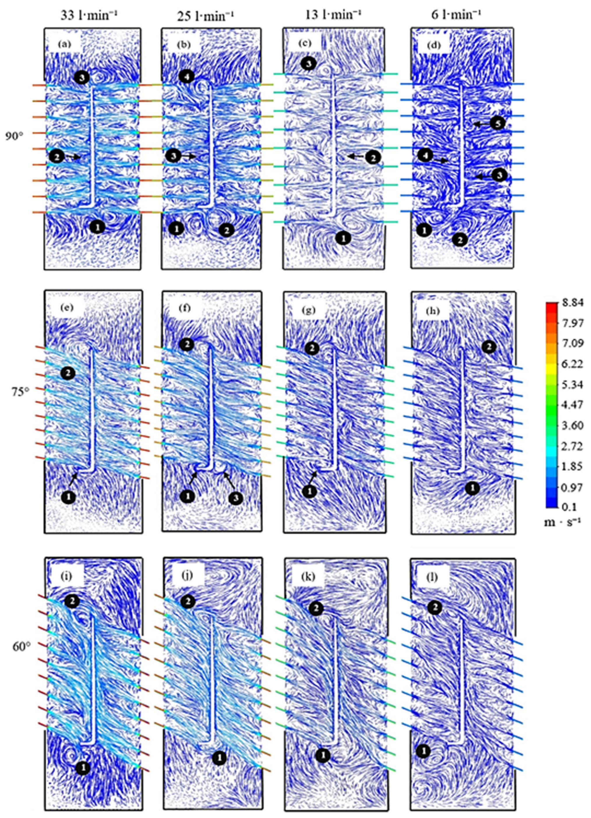
3.2. Fluid-Dynamic Fields

Angle Effect Analysis

Once the fluid-dynamic field of the mathematical model was validated, the numerical simulation was applied to study the effect on the fluid dynamics in the system by varying the arrangement of the stirring jets at 90°, 75° and 60°. The objective was to evaluate, through a stirred quenching heat treatment with recirculation of the cooling medium, the coverage of the jets in the quenching zone and the uniformity of the impact velocity to the probe. To estimate the first parameter, a longitudinal plane located 0.86 m from the bottom of the vessel, which cuts the first row of jets, was analyzed. Figure 5 shows the pathlines colored by magnitudes of velocity, varying the impact angle of 90°, 75° and 60°, as well as the water-flow rates. It can be seen that for the 90° angle in the four water flows, the coverage of the jets is uniform throughout the entire workpiece but, in some cases, it can be seen that when the jets impact, the fluid disperses to the sides after impact with the piece, that is, it collides with the flow of the adjacent jet and generates small recirculations, Figure 5a–d, which, although they do not deviate the direction of the fluid can cause areas of low velocity that can affect the thermal gradient at the time the piece is being quenched, depending on the variation in velocity in those areas.

On the other hand, when the jets are at 75°, better water-flow coverage is observed in the middle section of the piece, compared to the 90° angles for all flow rates. In addition, deviations of the jets are observed both in the upper and lower part of the piece, so the structure exhibited by the fluid is quite similar since an abrupt change derived from the variation in flow rate is not shown. Finally, at 60° can be seen better coverage of the fluid on the piece, unlike the 75° angle, which shows that the jets impact the piece axially, in Figure 5i,j,l, where it exhibits similar behaviors, showing that the jets do not cover the upper area of the piece. However, with the flow of 13 l·min⁻¹, Figure 5k, an area is evident where the piece is not covered in its lower part, ❶. To evaluate the uniformity of the impact velocity on the piece, this variable was quantified and averaged on the faces that receive the impact of the jets along the piece, that is, on the lateral faces. Figure 6 shows the graphs of the average velocity for the three jet angles and the four flows employed. It can be seen that as the flow increases, the velocity with which the piece is impacted is more significant; however, with the flow of 33 l·min⁻¹, many variations in velocity are shown along the impact area for the 90° angle, which could cause surface defects such as cracks in the piece, according to what has already been reported [30,31]. This oscillation also manifests for the angles of 75° and 60°, but the difference is that at the ends of the piece, the velocities are low due to the recirculations shown in Figure 5e,i. On the other hand, it is evident in Figure 6a–c that with this high flow, the impact velocities increase when the angle decreases; this effect is shown with the flow of 25 l·min⁻¹. The effect of the angle seems to have no effect using a flow of 13 l·min⁻¹ since the velocity is maintained at values between 0.3 and 0.5 m·s⁻¹, which would generate a more uniform heat extraction. Finally, for the lowest flow, there are slightly higher impact velocities with the 75° angle with values of around 0.2 m·s⁻¹, while at 90° and 60° very similar values are achieved between both with values around 0.1 m·s⁻¹, which indicates that the cooling rate will present similar magnitudes for the three cases, being more remarkable for the jets at 75° as will be seen in the Section 3.3.

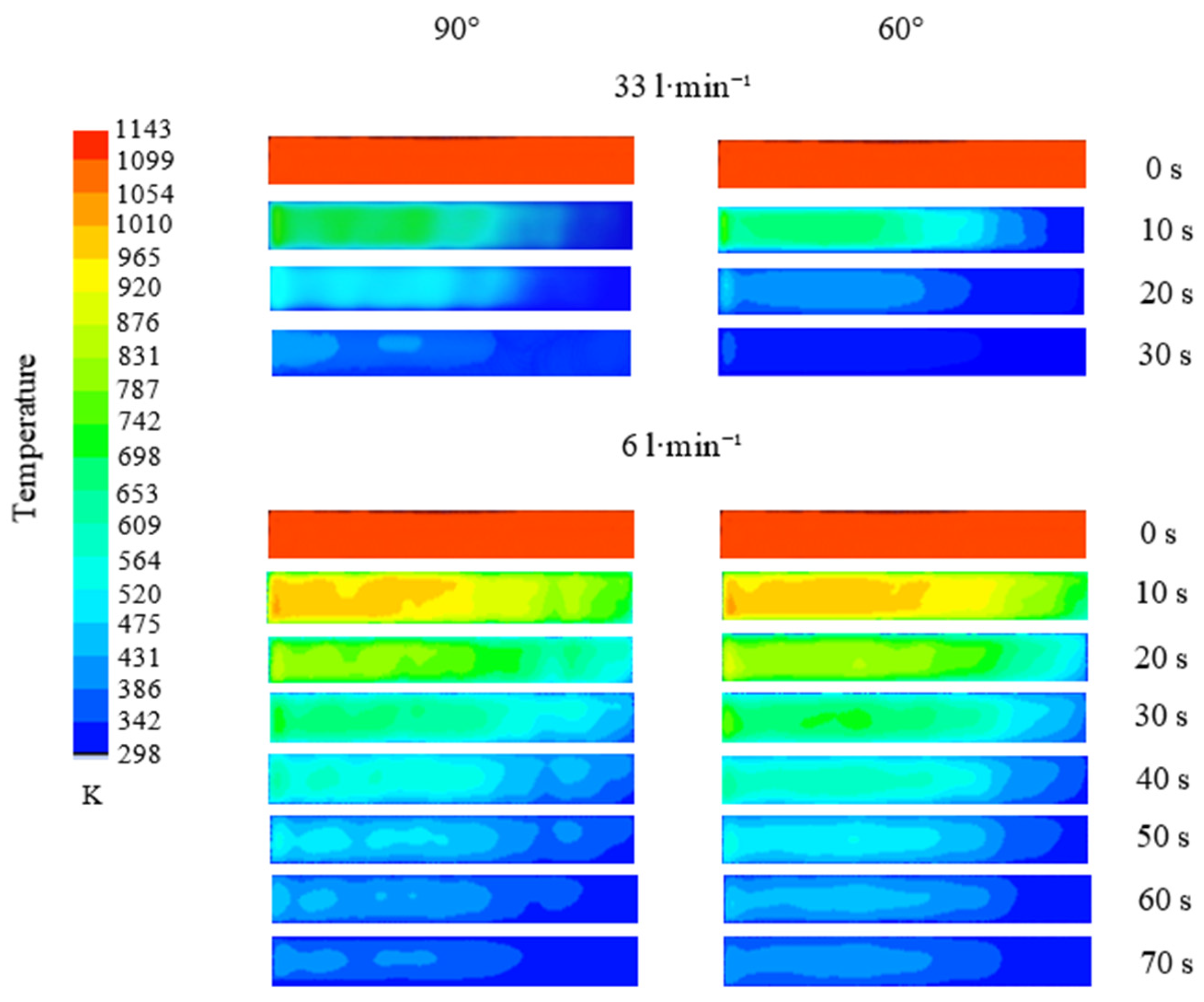
3.3. Thermal Analysis

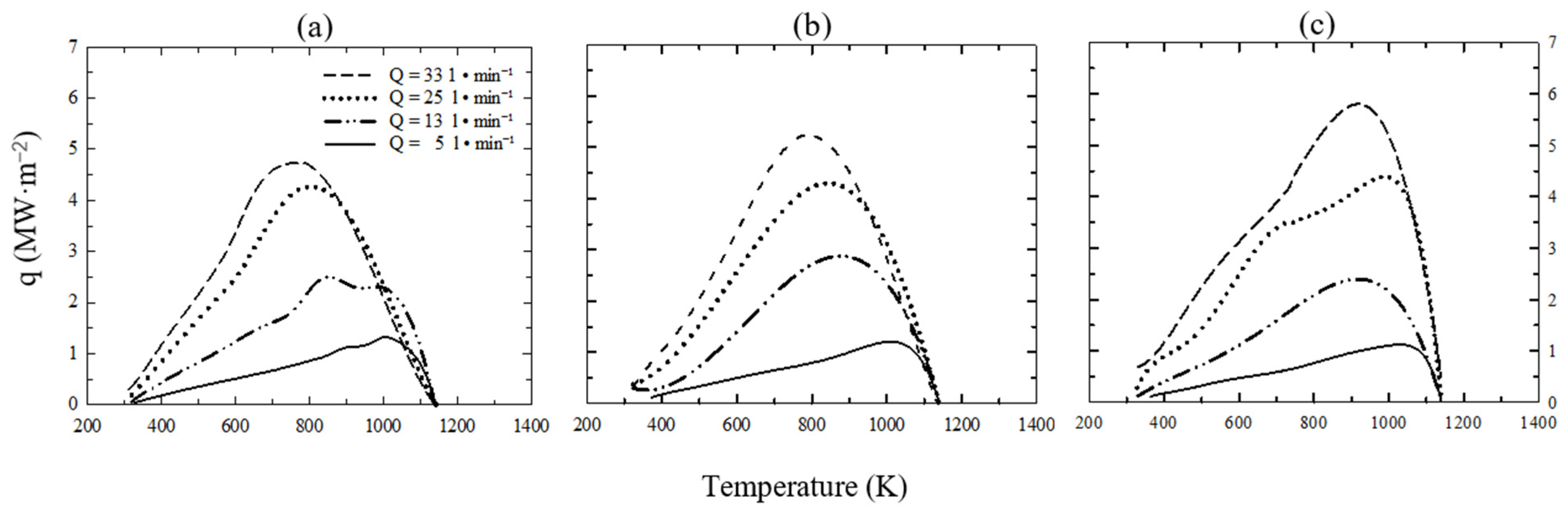
Figure 7 shows the comparison of the average cooling rates on the probe faces for the change in angle of the jets to 90°, 75° and 60° with the different flows used. In Figure 7a, which corresponds to a flow rate of 33 l·min⁻¹, it can be seen that higher heat extraction rates are achieved with the jet angle at 60° being ~323.59 K·s⁻¹, followed by the jets at 75° with a value of 271.70 K·s⁻¹, while at 90° lower cooling rates are reached, of 243.61 K·s⁻¹. As observed in Figure 6 for these cases, the greater the magnitude of the jet impact velocity, the faster the cooling occurs, as observed in [32]. Meanwhile, in Figure 7b, which corresponds to the flow of 25 l·min⁻¹, a trend similar to the case described above is observed for the three angles; that is, the cooling is faster with the angle 60° (255.82 K·s⁻¹), then the angle at 75° (238.36 K·s⁻¹) and finally 90° (215.20 K·s⁻¹). However, for this case, the difference between the values of the cooling rates is not as significant as with the previous flow, which is because the magnitude of the impact velocity remains in similar ranges for the three angles. On the other hand, Figure 7c shows some differences in the 90° angle concerning the other two angles since the value obtained is 123.57 K·s⁻¹ at a temperature of 1100 K, while the angles of 75° and 60° present a change in their trend to the other flow rates since higher heat extraction rates are achieved with the jets at 75° with a value of 156.6 K·s⁻¹ a temperature of 1075 K versus 149.06 K·s⁻¹ at 1059 K for the 60° angle. This behavior is because, as described in the Section 3.2 the configuration of the jets at 60° showed better uniformity of the impact velocity; a notable deviation of the jets was evident in the right part of the piece (see Figure 5c,k). Similarly, in Figure 7d, it can be seen that the cooling rate does not present notable changes that could influence the final properties of the piece for the three angles because the average impact velocities reached very similar values. Magnitudes of ~0.2 m·s⁻¹ for 75°, ~0.1 m·s⁻¹ for both cases 90° and 60° were obtained, so that with the angle of 75° higher cooling rates are achieved with a magnitude of ~73.52 K·s⁻¹, followed by the jets at 60° and 90° with ~63.98 K·s⁻¹ and 58.47 K·s⁻¹, respectively.

Figure 8 shows the thermal evolution of the probe through the temperature contours in a central-longitudinal plane of the steel piece for two angles of 90° and 60° with flows of 33 l·min⁻¹ and 6 l·min⁻¹ at different times. It can be seen that for more significant water flows, regardless of the angle used, the cooling of the piece is more severe. Additionally, it can be observed that the cooling is not uniform along the piece in all cases because it presents a gradual decrease in its thickness over its length, which causes faster cooling on its right side. Also, it can also be noted at different times that the cooling is seriously affected by the change in the angles of the jets, which shows that the impact of these on the hot surface and in the area where the probe has a constant section to cool with jets to 60° promotes more homogeneous heat extraction. Likewise, it is evident that at 90°, there are regions where the heat extraction is slightly more significant, which causes thermal gradients during the quenching treatment, the phenomenon being more notable with the flow at 33 l·min⁻¹ for 20 s and 30 s of cooling. In the thermal profiles with a flow of 6 l·min⁻¹, it can be noted that during cooling, the behavior is similar since the areas of the piece are in comparable temperature ranges, which indicates that the heat extraction does not present notable differences with low flows for the angles studied, which is in agreement with the data obtained from the average cooling rates, shown in Figure 7.

3.4. Boiling Curves

Figure 9a–c show the behavior of the heat fluxes to the surface temperature during the cooling of the workpiece for the jet angles at 90°, 75° and 60°, respectively. In the three impact angles, it can be seen that the higher the flows, the greater the heat extraction; however, the 60° angle offers higher heat extraction rates due to the fluid-dynamic behavior of the jets that cause higher impact velocities on the workpiece. Also, it can be seen that, at angles of 90° and 75°, the points of the critical heat flux (CHF) appear at different temperatures; that is, the higher the flow used, the lower the temperature where this CHF value is reached, as has already been reported [33]. For all cases, in the first moments of the cooling process, heat fluxes increase until reaching a maximum value. This phenomenon is due to the transition-boiling regime, where the suppression of the vapor layer occurs, giving rise to liquid–solid contact and extracting large amounts of heat since the higher the cooling rate, the greater the critical heat flow that is achieved. This behavior is because the fluid can absorb more thermal energy from the piece, which translates into more severe cooling. While for the water flow of 33 l·min⁻¹, the 60° angle reaches values of 5.8 MW·m⁻², the 75° angle reaches values of 5.23 MW·m⁻², and the 90° angle reaches values of 4.47 MW·m⁻². Subsequently, the heat fluxes begin to decrease as the surface temperature decreases, and thus, the nucleated boiling and convection regimes in a single phase are manifested in the curves. The curves with 25 l·min⁻¹ water flows follow the same trend with the angles at 90° and 75°. However, the behavior is different at 60°, since after reaching the maximum flow, it begins to decrease its value until reaching an inflection point right at the nucleated boiling stage at a value of 3.4 MW·m⁻² at a temperature of 724 K. This type of behavior in the boiling curves is manifested when the stirring jets exhibit an unstable behavior, that is, the direction of the fluid at the exit of the jets is deviated by time intervals during cooling, which implies that they do not constantly impact the piece. The same occurs with the angle at 90° and a flow rate of 13 lt·min⁻¹ except that at the beginning, it reaches a first maximum with a value of 2.3 MW·m⁻² at a temperature of 975.60 K, then shows a decrease in its value to 2.2 MW·m⁻² and increases again to 2.5 MW·m⁻² at a temperature of 844 K, to subsequently decrease gradually. With this last case, it can be inferred that at the beginning of cooling, the jets present variations in their direction, preventing them from impacting the probe in a constant mode until they stabilize, causing an increase in heat extraction. Finally, for the lower water flow of 6 l·min⁻¹, the heat flux values for the three jet angles remain very similar as expected, with values of 1.33, 1.27, and 1.22 MW·m⁻² for the angles of 75°, 60°, and 90°, respectively.

3.5. Effect of Stirring Velocity on Phase Transformation

To evaluate the effect of stirring the cooling medium on the phase transformations that occur in steel, tests were carried out with the scale model described in Figure 2. Two cases were studied: one without agitation of the cooling medium (0 l·min⁻¹) and another with a 9 l·min⁻¹ flow rate. Using the cooling (flow) conditions described, it aims to evaluate whether a notable microstructural change allows characterizing the properties obtained when 15B35H steel is quenched. Figure 10 shows the effect of stirring velocity on the microstructure of the heat-treated steel. As shown in Figure 10a, cooling the steel without stirring promotes the formation of ferrite, bainite and martensite in amounts of ~32.6%, 24.7% and 42.7%, respectively, according to what was calculated by ImageJ v.1.54d software. On the other hand, in Figure 10b, which corresponds to the sample cooled to 9 l·min⁻¹ with a jet impact angle of 90°, a considerable decrease in the amount of bainite and a significant increase of the martensite phase can be observed. Meanwhile, the ferrite level has been completely reduced. Although the quenching medium is the same for both samples, it can be observed that the agitation of the quenching medium does play a predominant role in the phase transformation. The microstructures obtained agree with what was calculated in the CCT diagram shown in Figure 11, which was obtained using JMatPro^® v.7.0 from the chemical composition and with an ASTM 9-grain size. The diagram shows two dashed lines; one in black corresponds to the cooling curve of (0 l·min⁻¹), and another red one belongs to the 9 l·min⁻¹ flow rate at 90°. According to what is shown in the diagram of Figure 11 and following the cooling curve without stirring, it can be observed that this condition crosses the transformation regions of the ferrite, bainite and martensite phases, which is in agreement with what is shown in Figure 10a.

In contrast, if impacted with water jets at 90° at 9 l·min⁻¹, the cooling rate achieved considerably decreases the formation of ferrite, allowing the phase transformation of γ→α′ as well as small amounts of bainite, since, as shown in Figure 11, the cooling curve (red dashed line) crosses the beginning of the transformation of this phase, in such a way that the microstructure is mainly made up of a mixture of α′+ B. On the other hand, according to what is shown in Figure 6, it can be seen that the higher the impact speed of the jet, the greater the cooling capacity, regardless of the angle used, which is associated with a more significant transformation to martensite, as shown in Figure 10b. However, the heat-extraction speed is a parameter that depends on the impact angle since, as shown in Figure 9, a greater heat extraction (q) is obtained when the angle used is 60° compared to the 90°, which would facilitate the γ→α′ phase transformation. However, the use of 90° jets ensures the uniformity of the fluid-dynamic field, as shown in Figure 5, thus allowing the cooling of the part uniformly, thus avoiding high thermal gradients in the quenched sample and, consequently, cracking of the material, which could ensure obtaining parts with good mechanical properties.

4. Conclusions

In this work, the effect of the flow and angle of the water jets in a quenching thermal treatment system on the heat transfer and phase transformation in boron steel pieces was successfully resolved through experimental and mathematical simulation, derived from the above, concludes the following:

• The fluid-dynamic field was satisfactorily validated using the PIV technique, as was the thermal behavior by calculating the transient coefficient h employing the inverse heat conduction method, this allowed our computational model to perform surface heat-flow calculations in the quenching process of steel parts by modifying the operating parameters such as impact angle and flow velocity.
• It was found that the correlation used in the software correctly resolves the heat transfer rate due to convective cooling since it takes into account the velocity with which the fluid impacts the piece, which avoids carrying out experiments for each condition.
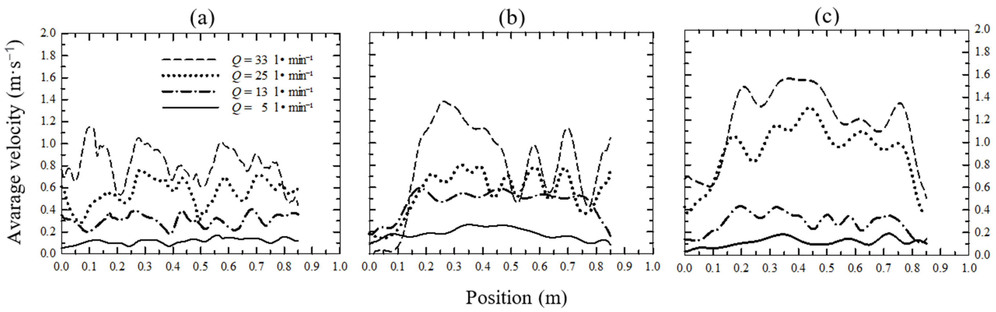
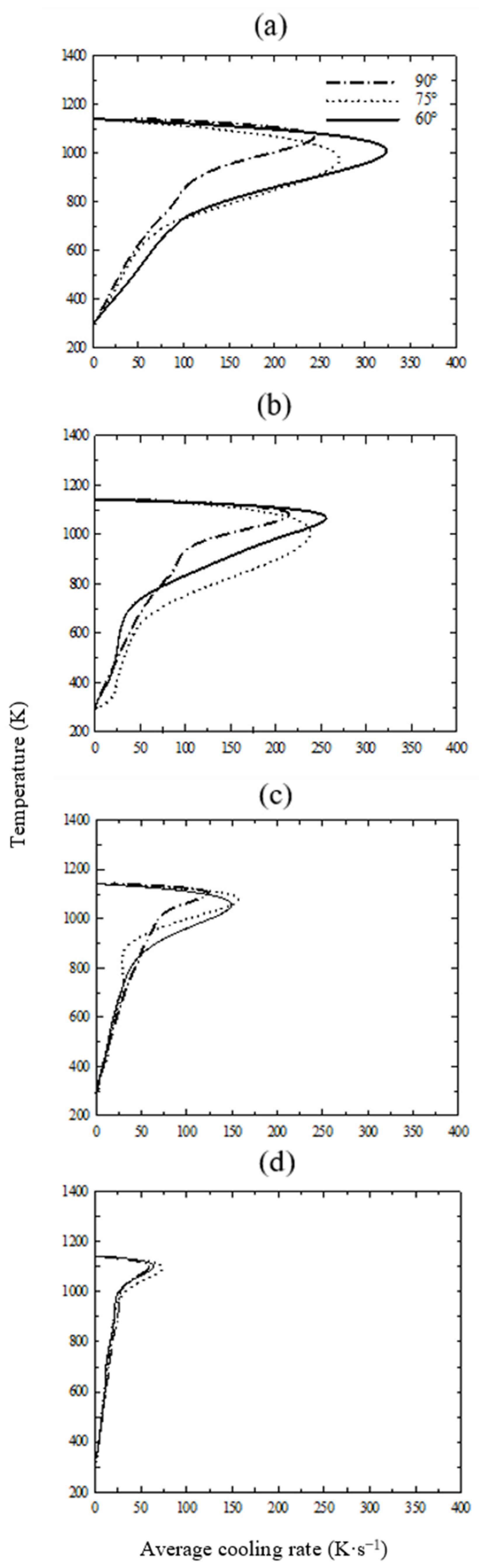
• The jet angle of 60° generates greater heat extraction at high injection flows of ~33 l·min⁻¹; this is due to the flow behavior since the orientation of the jet promotes high-impact velocities throughout the probe, capable of causing high-velocity gradients and which generate non-uniform cooling of the part, which would promote its cracking. On the other hand, at low water flows, the impact angle does not significantly affect heat transfer since, as could be observed, the heat-extraction rates remained similar.
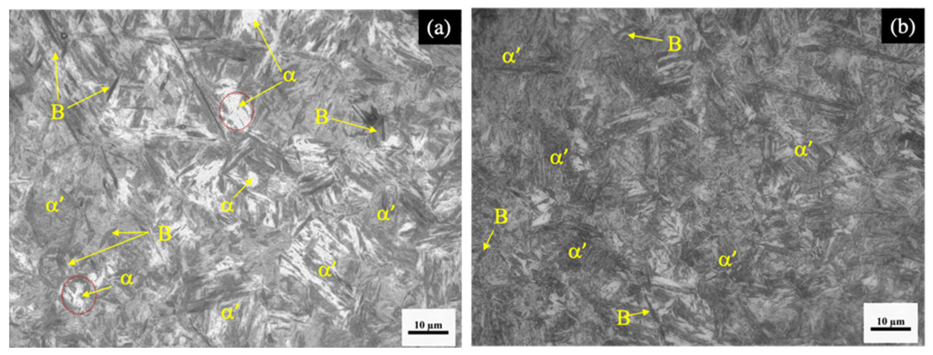
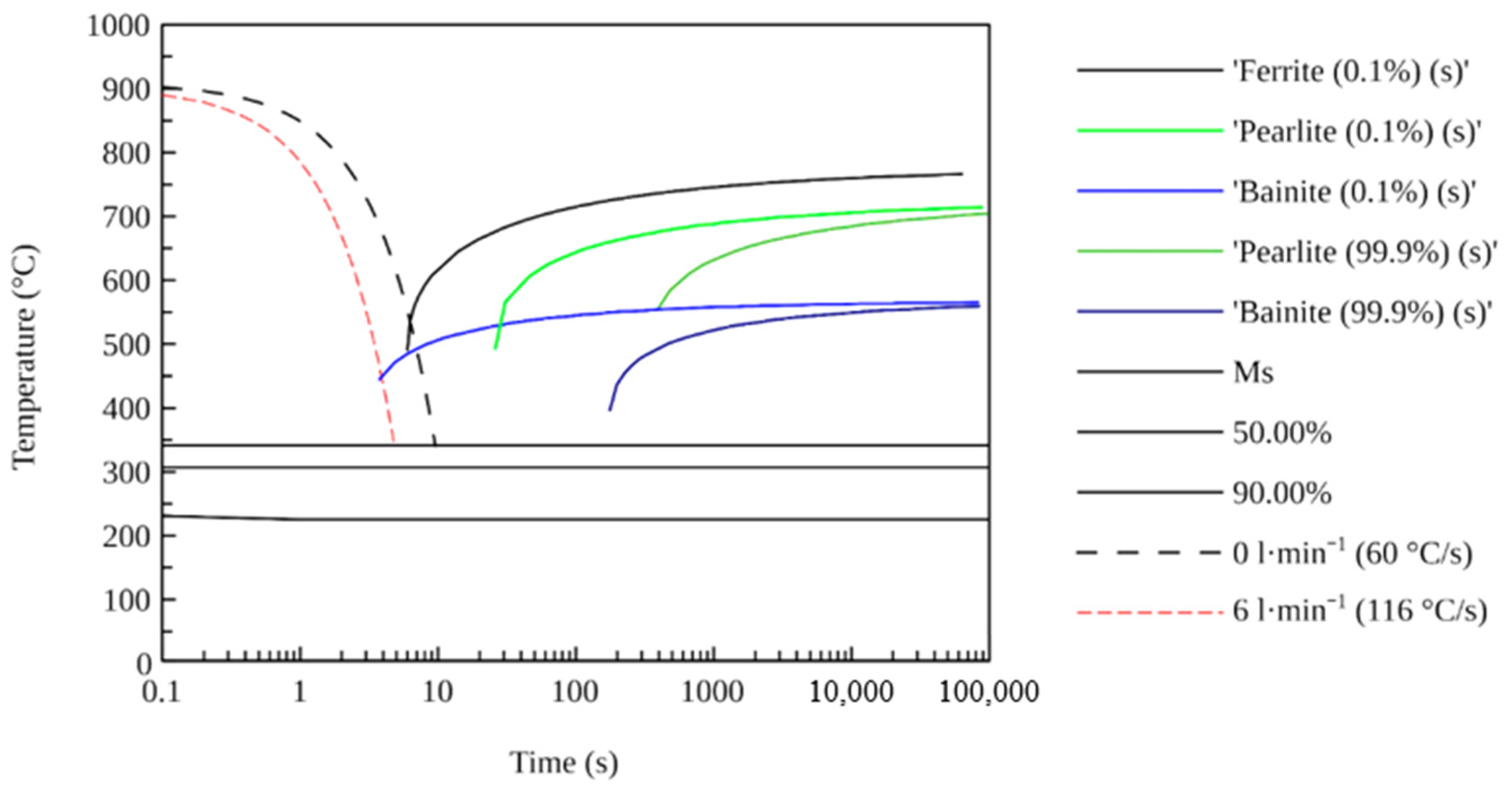
• It was found in the physical tests that the transition from an agitation of 0 l·min⁻¹ to one of 6 l·min⁻¹ produced by the jets during quenching generates significant microstructural changes due to obtaining extraction rates of higher heat levels that promote the formation of bainite and martensite, inhibiting the formation of ferrite independently of the jet angle.

References

1. Hernández-Morales, B.; Vergara-Hernández, H.J.; Solorio-Díaz, G. Fluid dynamics during forced convective quenching of flat-end cylindrical probes. In Proceedings of the 8th WSEAS International Conference on Fluid Mechanics, 8th WSEAS International Conference on Heat and Mass Transfer, Puerto Morelos, Mexico, 29–31 January 2011; pp. 135–141. [Google Scholar]
2. Kumar, A.; Metwally, H.; Paingankar, H.; MacKenzie, S. Evaluation of flow uniformity around automotive pinion gears during quenching. In Proceedings of the 5th International Conference on Quenching and Control Distortion at 2007 European Conference on Heat Treatment, Berlin, Germany, 25–27 April 2007; pp. 1–8. [Google Scholar]
3. Xia Wei, Y.; Jing Chuan, Z.; Dong, H.; Zhong Hong, L.; Zhi Sheng, N.; Yong, L. Optimum design of flow distribution in quenching tank for heat treatment of A357 aluminum alloy large complicated thin-wall workpieces by CFD simulation and ANN approach. Trans. Nonferrous Met. Soc. China 2013, 23, 1442–1451. [Google Scholar]
4. Garwood, D.R.; Lucas, J.D.; Ward, J. Modeling of the flow distribution in an oil quench tank. JMEP 1992, 1, 781–788. [Google Scholar] [CrossRef]
5. Chen, N.; Liao, B.; Pan, J.; Li, Q.; Gao, C. Improvement of the flow rate distribution in quench tank by measurement and computer simulation. Mater. Lett. 2006, 60, 1659–1664. [Google Scholar] [CrossRef]
6. Bogh, N. Quench tank agitation design using flow modeling. In Proceeding of the International Heat Treating Conference: Equipment and Processes, Schaumburg, IL, USA, 18–20 April 1994; Totten, G.E., Wallis, R.A., Eds.; ASM International: Materials Park, OH, USA, 1994; pp. 51–54. [Google Scholar]
7. Kernazhitskiy, S.L.; Recktenwald, G. Numerical modeling of a flow in a large quench tank. In Proceeding of the ASME 2004 Heat Transfer/Fluids Engineering Summer Conference, Charlotte, NC, USA, 11–15 July 2004; pp. 129–137. [Google Scholar]
8. Halva, J.; Volley, J. Modeling the flow in a quench bath. Hut. Listy 1993, 48, 30–34. [Google Scholar]
9. Xia Wei, Y.; Jing Chuan, Z.; Wen Ya, L. CFD-supported optimization of flow distribution in quench tank for heat treatment of A357 alloy large complicated components. Trans. Nonferrous Met. Soc. China 2015, 25, 3399–3409. [Google Scholar]
10. Madireddi, S.; Nambudiripad-Krishnan, K.N.; Satyanarayana-Reddy, A.S. Numerical Analysis of Heat Transfer during Quenching Process. J. Int. Eng. India Ser. 2016, 99, 217–222. [Google Scholar] [CrossRef]
11. Li, J.; Zhao, X.; Zhang, H.; Li, D. Numerical simulation of single–jet impact cooling and double-jet impact cooling of hot-rolled L-shaped steel based on multiphase flow model. Sci. Rep. 2024, 14, 4965. [Google Scholar] [CrossRef] [PubMed]
12. Fátima-Gomes, D.; Parreiras-Tavares, R.; Martins-Braga, B. Mathematical model for the temperature profiles of steel pipes by water cooling rings. J. Mater. Res. Technol. 2019, 8, 1197–1202. [Google Scholar] [CrossRef]
13. Kobayashi, K.; Haraguchi, Y.; Nakamura, O. Water Quenching CFD (Computational Fluid Dynamics) Simulation with Cylindrical Impinging Jets. Nippon. Steel Sumitomo Met. Tech. Rep. 2016, 401, 105–110. [Google Scholar]
14. Liu, Z.; Jie, Y.; Li, S.; Nie, W.; Li, L.; Guan, W. Study on inhomogeneous cooling behavior of extruded profile with unequal and large thicknesses during quenching using thermo-mechanical coupling model. Trans. Nonferrous Met. Soc. China. 2020, 30, 1211–1226. [Google Scholar] [CrossRef]
15. Rok, K.; Leopold, Š.; Matjaž, H.; Dongsheng, Z.; Bernhard, S.; David, G. Numerical simulation of inmersion quenching process for cast aluminium part at different pool temperatures. Appl. Therm. Eng. 2014, 65, 74–84. [Google Scholar]
16. Bouaichaoui, Y.; Končar, B. Numerical and experimental investigation of convective flow boiling in vertical annulus using CFD code: Effect of mass flow rate and wall heat fluxes. Ann. Nucl. Energy 2023, 181, 109514. [Google Scholar] [CrossRef]
17. Husain, S.; Altamush, M.; Ahmad, S. Effect of geometrical parameters on natural convection of water in a narrow annulus. Prog. Nucl. Energy 2019, 112, 146–161. [Google Scholar] [CrossRef]
18. Coras, C.; Martín, E.B. Modeling and numerical simulation of the quenching heat treatment application to the industrial quenching of automotive spindles. In Advances on Links between Mathematics and Industry; Springer: Cham, Switzerland, 2021; Volume 15. [Google Scholar]
19. Rauch, L.; Zalecki, W.; Kuziak, R.; Garbarz, B.; Raga, K.; Bzowski, K.; Pietrzyk, M. Numerical simulations of aircraft engine ring gear quenching by using mean field model of phase transformations in Pyroware steel 53. J. Aerosp. Eng. 2023, 36, 04023079. [Google Scholar] [CrossRef]
20. Wang, J.; Yang, S.; Li, J.; Ju, D.; Li, X.; He, F.; Li, H.; Chen, Y. Mathematical simulation and experimental verification of carburizing quenching process based on multi-field coupling. Coatings 2021, 11, 1132. [Google Scholar] [CrossRef]
21. Mehran, G.; Ali, A.R.; Abas, R. Heat transfer and uniformity enhancement in quenching process of multiple impinging jets with Newtonian and non-Newtonian quenchants. Int. J. Therm. Sci. 2019, 142, 220–232. [Google Scholar]
22. Jiyuan, T.; Guan-Heng, Y.; Chaoqun, L. Computational Fluid Dynamics a Practical Approach, 3rd ed.; Butterworth-Heinemann: Oxford, UK, 2018; pp. 192–203. [Google Scholar]
23. Muhammad, J.; Aqib, M.K.; Munish, K.G.; Mozammel, M.; Ning, H.; Liang, L.; Vinothkumar, S. Influence of CO2-snow and subzero MQL on thermal aspects in the machining of Ti-6Al-4V. Appl. Therm. Eng. 2020, 177, 115480. [Google Scholar]
24. Muhammad, J.; Ning, H.; Wei, Z.; Liang, L.; Munish, K.G.; Murat, S.; Aqib, M.K.; Rupinder, S. Heat transfer efficiency of cryogenic-LN2 and CO2-snow and their application in the turning of Ti-6Al-4V. Int. J. Heat Mass Transf. 2021, 166, 120716. [Google Scholar]
25. Beck, J.V. User’s Manual for CONTA: Program for Calculating Surface Heat Fluxes from Transient Temperature Inside Solids; Technical Report; United States Michigan State University: East Lansing, MI, USA, 1983. [Google Scholar]
26. Beck, J.V.; Blackwell, B.; Haji-Sheikh, A. Comparison of some inverse heat conduction methods using experimental data. Int. J. Heat Mass Transf. 1996, 39, 3649–3657. [Google Scholar] [CrossRef]
27. Hernandez-Morales, B.; Brimacombe, J.; Hawbolt, E. Application of inverse technique to determine heat transfer coefficients in heat-treating operations. J. Mater Eng. Perform 1992, 1, 763–771. [Google Scholar] [CrossRef]
28. Farrera-Buenrostro, B.; Hernández-Bocanegra, C.A.; RamosBanderas, J.A.; Molina-Valdovinos, L.E.; López-Granados, N.M.; Vapalahti, S. Experimental study of the effect of the concentration of water/polyalkylene glycol solutions on heat transfer in steels subjected to quenching. Mater. Res. Express 2024, 11, 016515. [Google Scholar] [CrossRef]
29. Zuckerman, N.; Lior, N. Impingement heat transfer: Correlations and numerical modeling. J. Heat Transf. 2005, 127, 544–552. [Google Scholar] [CrossRef]
30. Canale, C.F.; Totten, G.E. Overview of distortion and residual stress due to quench processing part 1: Factors affecting quench distortion. Int. J. Mater. Prod. Technol. 2005, 33, 797–807. [Google Scholar] [CrossRef]
31. Karwa, N. Experimental Study of Water Jet Impingement Cooling of Hot Steel plates. Doctoral Thesis, Darmstadt: Technische Universitat Darmstadt, Frankfurt, Germany, 2012. [Google Scholar]
32. Li, X.; Xia, W.; Yang, K.; Dai, L.; Wang, F.; Xie, Q.; Cai, J. Quench cooling of steel plates by reciprocating moving water jet impingement. Exp. Therm. Fluid Sci. 2024, 153, 111127. [Google Scholar] [CrossRef]
33. Babu, K.; Kumar, P. Mathematical modeling of surface heat flux during quenching. Metall. Mater. Trans. B. 2010, 41, 214–224. [Google Scholar] [CrossRef]
Figure 1. (a) Isometric view of the computational domain of the quenching system with the variation of the jets angle. Workpiece dimensions of the computational domain (b) front view, (c) lateral view.
Fluids 09 00089 g001
Figure 2. Experimental Setup; (a) data acquisition system for thermal field (b) PIV system (c) Jets arrangement design.
Fluids 09 00089 g002
Figure 3. Fluid-dynamics validation, (a) numerical simulation, (b) PIV and (c) cross-sectional plane y-y’ of the quenching bath from mathematical modeling.
Fluids 09 00089 g003
Figure 4. Comparison of the estimated cooling curves with the mathematical and experimental model.
Fluids 09 00089 g004
Figure 5. Pathlines colored by velocity magnitude along the plane-zx at 0.86 m for the different water flows and jet angles. For 90° (ad), for 75° (eh), and for 60° (il).
Fluids 09 00089 g005
Figure 6. Averaged impingement velocity distribution along the lateral walls of the workpiece. (a) 90°, (b) 75° and (c) 60°.
Fluids 09 00089 g006
Figure 7. Cooling-rate behavior for the different jet angles and water flows studied; (a) 33 l·min−1, (b) 25 l·min−1, (c) 13 l·min−1, (d) 6 l·min−1.
Fluids 09 00089 g007
Figure 8. Profiles of thermal evolution obtained during cooling at 90° and 60° jets angles and flows of 33 l·min−1 and 6 l·min−1.
Fluids 09 00089 g008
Figure 9. Boiling curves from the numerical simulations for the jets angles of: (a) 90°, (b) 75° and (c) 60° at the different water flows studied.
Fluids 09 00089 g009
Figure 10. Effect of jets water flow on the phase transformation of 15B35H steel. (a) 50X nital 3%; 0 l·min−1, (b) 50X nital 3%; 6 l·min−1. α = ferrite, α′ = martensite, B = bainite.
Fluids 09 00089 g010
Figure 11. CCT diagram for 15B35H steel.
Fluids 09 00089 g011