Article

A Compressible Formulation of the One-Fluid Model for Two-Phase Flows

Laboratoire MSME, CNRS UMR 8208, Université Gustave Eiffel, 5 Boulevard Descartes, 77454 Marne-la-Vallée, France
*
Author to whom correspondence should be addressed.
Fluids 2024, 9(4), 90; https://doi.org/10.3390/fluids9040090
Submission received: 1 February 2024 / Revised: 13 March 2024 / Accepted: 10 April 2024 / Published: 12 April 2024
(This article belongs to the Section Mathematical and Computational Fluid Mechanics)

Abstract

:
In this paper, we introduce a compressible formulation for dealing with 2D/3D compressible interfacial flows. It integrates a monolithic solver to achieve robust velocity–pressure coupling, ensuring precision and stability across diverse fluid flow conditions, including incompressible and compressible single-phase and two-phase flows. Validation of the model is conducted through various test scenarios, including Sod’s shock tube problem, isothermal viscous two-phase flows without capillary effects, and the impact of drops on viscous liquid films. The results highlight the ability of the scheme to handle compressible flow situations with capillary effects, which are important in computational fluid dynamics (CFD).

1. Introduction

The modelling and simulation of two-phase compressible flows is a highly dynamic field of study due to their crucial involvement in energy systems, such as aerospace engineering, the oil and gas industry, nuclear and biomedical engineering, geophysical studies, and chemical processes.
The use of numerical simulation proves necessary for analysing and understanding compressible two-phase flows involving separated phases. Firstly, these flows are intrinsically complex and involve challenging interactions that occur between different phases of fluids or gases, particularly in the vicinity of interfaces. Additionally, safety considerations also drive the use of the numerical simulation. In applications like nuclear reactors or chemical processes, conducting experiments may not be safe or feasible. Further, the numerical simulation facilitates parametric studies, enabling engineers to efficiently explore a large range of operating conditions and design parameters. The reasons mentioned above have prompted the CFD community to develop a two-phase compressible flow model throughout the last few decades. Our efforts have been directed towards encompassing a wide array of Mach formulations documented in prior research. Noteworthy references include the work of [1,2,3,4,5,6] and other relevant sources.
In this paper, a compressible formulation is developed to simulate such flow situations. In this formulation, we solve the conservation of mass (in two forms), momentum, and total energy in each of the two phases, as well as an equation for the volume fraction. To close the system of equations, an equation of state is used to take into account the variations in density as a function of pressure and possibly temperature. The original formulation was introduced by [7] and recently extended to all-Mach flows by [8] to account for heat diffusion between two different compressible phases. In the present work, we extend this formulation by maintaining a strong coupling between velocity and pressure variables through the use of a monolithic solver [9,10,11] and by preserving the consistency between mass transport and momentum via a momentum-conserving scheme [12]. Our approach is different from what is traditionally performed in the two-phase compressible flow simulation community, for example Abgrall [13], Saurel [14], Massot [15], who use conservative variables such as density or momentum to solve the problem. The interest of our approach is to manage continuous quantities as long as no shock waves occur on velocity or pressure.
The remainder of this manuscript is structured as follows: Section 2 introduces the governing equations, including the conservation of mass, momentum, and total energy in each of the two phases. Section 3 describes the employed numerical schemes as well as the monolithic solver used for the solution of the saddle point system on the velocity–pressure coupling. In Section 4, we introduce different cases to check how accurate the incorporation of our compressible formulation is. These test cases are divided into two parts: one to deal with an adiabatic case for an inviscid flow, such as Sod’s shock tube problem, whereas a second part will be devoted to isothermal cases for viscous flows, like liquid injection in a closed cavity, the compression of an air bubble by water, and the drop impact on viscous liquid film. Ultimately, we will sum up our work and offer a perspective on future research.

2. Governing Equations

The derivation of the compressible formulation follows the work of [7]. The governing equations, suitable for modelling compressible two-phase flows using a one-fluid model, are presented. In their conservative forms, the mass and momentum equations read as follows:
ρ t + · ρ v = 0
and
ρ v t + · ρ v v = p + · τ ¯ ¯ + ρ g + F s
where v is the fluid velocity, p is the pressure field, t is the time, and ρ and μ are the properties of the fluid. In addition, τ ¯ ¯ = μ ( v + ( v ) T ) 2 3 μ · v is the viscous stress tensor and g is the gravity acceleration, whereas F s is the capillary term acting on the interface, modelled in this study by the continuum surface tension force (CSF) [16]. The tracking of the spatio-temporal evolution of the interface requires solving an advection equation for the phase indicator color function C:
C t + v · C = 0
By definition, C = 1 in one phase and 0 in the other phase. In the framework of a finite volume approximation of the solution, the color function in the control volumes cut by the interface is, for example, 0 < C < 1 . As the velocity and the pressure fields are coupled, a relation between v and p is needed to obtain the evolution equation for the pressure. Thereby, the conservation of mass equation is not used in its original form (Equation (1)) but is transformed into a pressure equation that is combined with the velocity variable. Within the framework of a compressible flow between two successive instants t and t + d t , the differential in the density with respect to the pressure p and the temperature T leads to
d ρ d t = ρ p T d p d t + ρ T p d T d t
Introducing the coefficients of isothermal compressibility and isobaric thermal expansivity (sometimes called the expansion or dilatation coefficient), χ T = ρ 1 ρ / p T and β = ρ 1 ρ / T p , respectively, the mass conservation (Equation (1)), combined with Equation (4), can be rewritten as
χ T d p d t + β d T d t + · v = 0
For incompressible ( χ T = 0 ) and isothermal ( β = 0 ) flows, Equation (5) gives · v = 0 .
When considering compressible flow, the energy equation is also addressed. Within the scope of this paper, we focus on scenarios where thermal diffusion and mass transfer at the interface do not play a significant role and are then neglected. Consequently, under these specific circumstances, the total energy equation is formulated as follows:
ρ e t + · ρ e v = · v p + · τ ¯ ¯ · v + ρ g · v + F s · v
where e = u + e k denotes the total energy, which is the sum of the internal energy u and kinetic energy per unit mass e k = v 2 / 2 .
To complete the set of equations, an equation of state (EoS) that establishes a relationship among the thermodynamic variables, pressure, p; density, ρ ; and temperature, T, is required. For any phase, gas or liquid, the Noble–Abel Stiffened-Gas (NASG) equation [17] can give the general formulation of an EoS. In this work, the liquid phase is always assumed to be incompressible, while the ideal gas model is adopted for the gas phase. The variation in the density as a function of pressure and temperature is classically expressed by ρ = p / ( r T ) , wherein r is the specific gas constant. On the other hand, from the NASG EoS of an ideal gas, it is seen that ρ = p / ( u γ 1 ) , with γ = c p / c v as the isotropic gas coefficient. The combination of the two previous expressions provides a relation for the temperature as a function of the internal energy, T = r u ( γ 1 ) , needed to close the system of Equations (2), (5) and (6), where the interface dynamics are provided by Equation (3).

3. Numerical Scheme

In this section, the global algorithm used to solve the coupled mass, momentum, and energy equations detailed in the previous section is presented.
The algorithm was designed with the underlying idea of a fully implicit formulation of system equations. For example, in momentum conservation Equation (2), all variables ( ρ , v , …) and terms would like to be resolved simultaneously. Due to non-linearity, some quantities, such as physical properties, the inertial term, or the geometrical properties of the interface, are estimated with values expected to closely approximate those obtained through implicit solving. To that purpose, a consistent reformulation and discretization of the inertial term, based on a momentum preserving approach [12], is used. The spacial discretization relies on a classical conservative finite volume approach and is not detailed in this paper. In practice, solving the full system introduces a sequential resolution of equations that themselves combine explicit variables (inertial contribution) with implicit variables resolved by the inversion of linear systems.
After time discretization, all variables at time t n = t 0 + n Δ t , where n is the iteration number and Δ t the constant (non restrictive) time step, are supposed to be known from a previous solution, directly ( v n , p n , C n , and e n ) or from a reconstruction ( ρ n , μ n , …). At this step, density and, more generally, all the physical properties are synchronised with the phase indicator function C n . The density is, for example, deduced from a mixing rule, ρ n = ( 1 C n ) ρ 1 + C n ρ 2 , where ρ i is the density of phase i. According to the phase state, an EoS is used to specify the behaviour of ρ i .
  • The initial step involves the inertial term computation of Equations (2) and (6). As the l.h.s. of the mentioned equations has the same mathematical structure ϕ / t + · ( ϕ v ) , with ϕ = ρ v , ρ e , a general approach is used to compute temporary variables (denoted ϕ ) in the operator splitting framework [12]. As the density is also a required variable, Equation (1) is also used in the numerical scheme in order to provide an approximation of the density.
    In practice, ϕ n = ρ n , ρ n v n , ρ n e n is first initialised before the time integration using a third-order accurate strong stability preserving Runge–Kutta (SSP-RK3) time integrator [18]:
    ϕ ( 1 ) = ϕ n Δ t · ϕ n v n
    ϕ ( 2 ) = 3 4 ϕ n + 1 4 ϕ ( 1 ) 1 4 Δ t · ϕ ( 1 ) v a d v ( 1 )
    ϕ = 1 3 ϕ n + 2 3 ϕ ( 2 ) 2 3 Δ t · ϕ ( 2 ) v a d v ( 2 )
    where v a d v ( 1 ) = 2 v n v n 1 and v a d v ( 2 ) = ( 3 v n v n 1 ) / 2 are the velocities correctly extrapolated to maintain scheme accuracy [19]. To ensure that ϕ remains bounded during advection, high-order schemes such as CUI, WENO, or even CUBISTA are used (see [19] and the references herein for more details).
    At the end of this step, discrete consistency between the temporary density, ρ ; momentum, ( ρ v ) ; and energy, ( ρ e ) variables is ensured. Furthermore, as Equation (1) is a pure advection equation, ρ directly provides a predicted density: ρ n + 1 = ρ .
  • The next step consists of the color function C advection. A conservative VOF approach, proposed by [20], is used where Equation (3), with time discretization, is formulated as
    C n + 1 C n Δ t + · C n v a d v ( 2 ) = C n · v a d v ( 2 )
  • With the knowledge of C n + 1 , the termophysical properties of the one-fluid model are updated. For ξ = μ , χ T , β , γ , and r, by using an arithmetic mixing law,
    ξ n + 1 = 1 C n + 1 ξ 1 + C n + 1 ξ 2
    where ξ i denotes the property corresponding to phase i. Note that the density is not updated as its value is already known from step 1.
  • The geometrical properties, normal properties n , and curvature κ , of the interface are evaluated. Here, a smoothed color function C ˜ n + 1 is computed from a diffusion step applied on C n + 1 and the definition
    n n + 1 = C ˜ n + 1 C ˜ n + 1 a n d κ n + 1 = · n n + 1
    can be used in the CSF expression of F s = σ κ n δ I where σ is the surface tension and δ I is the interface localisation.
  • From the EoS of an ideal gas, the temperature T can be expressed as a function of the solved variables v and e,
    T = γ 1 r e v 2 2
    and can be injected into the mass conservation (Equation (5)) that couples solved quantities v , p, and e. However, the velocity norm prevents an implicit coupling due to the non-linearity. The total derivative d T / d t will then be made explicit in the following for non isothermal flows.
  • Using the new density ρ n + 1 and the temporary momentum ( ρ v ) from step 1, the physical and interface properties from steps 3 and 4, and the temperature definition from step 5, the mass conservation, augmented by the compressibility and dilatation effects, and the momentum equations read, with a first-order time discretization,
    χ T n + 1 p n + 1 p n Δ t + v n + 1 · p n + β n + 1 T n T n 1 Δ t + v n + 1 · T n + · v n + 1 = 0
    ρ n + 1 v n + 1 ( ρ v ) Δ t = p n + 1 + · τ ¯ ¯ n + 1 + ρ n + 1 g + σ κ n + 1 n n + 1 δ I
    where only the velocity v n + 1 and pressure p n + 1 fields are implicity coupled and constitute the unknown vector of the underlying linear system. This latter is solved with a BiCGStab(2) solver [21], where an efficient block triangular preconditioner, improving the convergence of the iterative solver as explained in [10,11], is used.
    A last discussion concerns the linearization of the term v n + 1 p n + 1 into v n + 1 p n . This choice relies essentially on the available stencils from the incompressible version of the used solver [11]. Another approach, where v n + 1 ϕ n + 1 , with ϕ being the pressure or the temperature field, is one again approximated with the application of step 1 to a conservative evolution equation for ϕ , is also considered.
  • Finally, we update the total energy ( ρ e ) n + 1 using the intermediate total energy ( ρ e ) computed in step 1 and all other variables now known at time t n + 1 :
    ( ρ e ) n + 1 ( ρ e ) Δ t = · v n + 1 p n + 1 + · τ ¯ ¯ n + 1 · v n + 1 + ρ n + 1 g · v n + 1 + σ κ n + 1 n n + 1 · v n + 1 δ I
    The total energy at the end of the time iteration is deduced from e n + 1 = ( ρ e ) n + 1 / ρ n + 1 .

4. Results

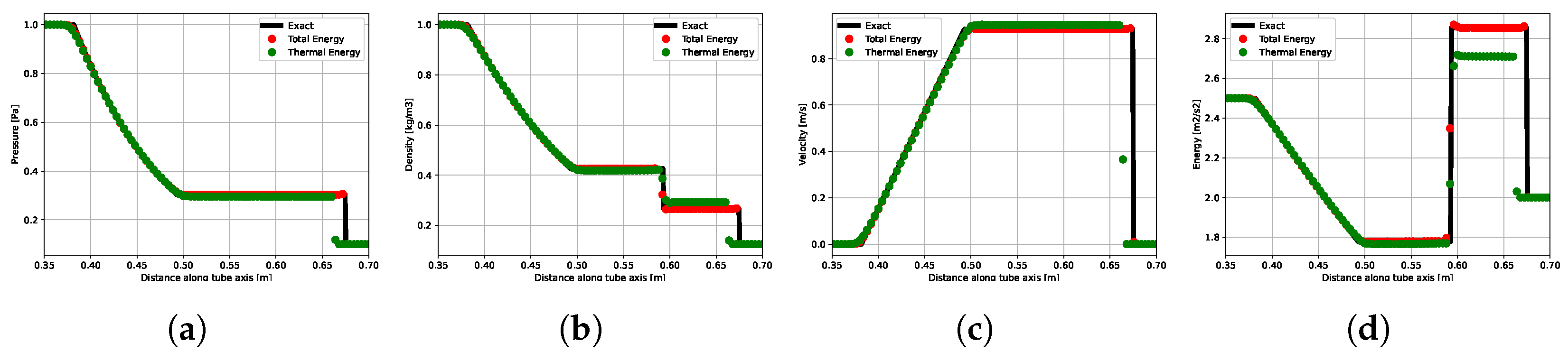
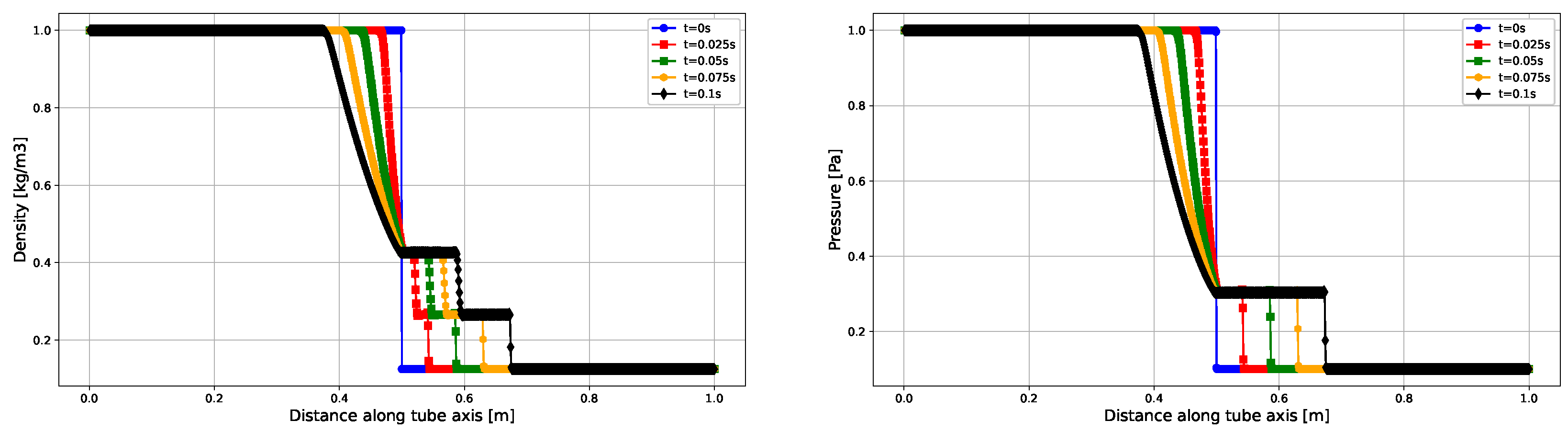
4.1. Sod’s Shock Tube Problem

This configuration was first introduced by [22]. This is a famous test case used to check the ability of the compressible schemes to avoid numerical instability at the shock level and improve the capture of a complex system of shock waves inside the tube. The governing equations are the Euler equations (Equations (12a) and (12b) with μ = 0 ) supplemented by the equation for the conservation of total energy (Equation (6)), with air characterized by an ideal gas model.
Here, a tube of length L = 1 m is considered. A membrane splits the tube into two regions: a high-pressure gas ( p l e f t , ρ l e f t ) on the left side and a low-pressure gas ( p r i g h t , ρ r i g h t ) on the other. The membrane is removed at time t = 0 . A complex system of shock waves develops inside the tube, i.e., an expansion wave, a contact discontinuity, and a normal shock wave.
The initial condition is given on the 1D computational domain, 0 x 1 m, as follows:
ρ , v , p = ρ l e f t , v l e f t , p l e f t = 1 , 0 , 1 if x 0.5 ρ r i g h t , v r i g h t , p r i g h t = 0.125 , 0 , 0.1 if x > 0.5
Preliminary studies were conducted to determine the appropriate mesh sizes for effectively capturing the phenomena of the shock tube. The simulations were carried out on a 250, 500, and 1000 Cartesian grid with time step conditions such that the CFL is defined by max | u | Δ t / Δ x = 0.3 . The matrices resulting from the discretization will be solved with the BiCGSTAB(2) solver with a residual of ε = 10 9 .
Figure 1 demonstrates well-resolved shocks with correct shock locations and fewer smeared contact discontinuities. The corresponding solutions show the evolution of pressure and density at different times ( 0 s , 0.025 s , 0.05 s , 0.075 s , and 0.1 s ) as a function of the curvilinear abscissa of the shock tube. From this figure, it is clear that an expansion wave propagates to the left, a shock wave propagates to the right, and there is discontinuity between these two waves.
Since the analytical solution was available, the theoretical curves are overlayed on the numerical ones in Figure 2. This illustrates a clear convergence of the numerical simulations to the exact solution when using a total energy equation, whether for velocity, pressure, internal energy, or density.
Finally, the choice of the solved energy equation is discussed here. As mentioned in Section 3, as the total energy conservation is used, the temperature is deduced from the fluid EoS properties. Other choices are possible, such as enthalpy conservation or, in a more traditional way, the energy equation formulated with the temperature variable (heat or thermal energy equation). The two first choices involve dealing with conserved quantities, i.e., the total energy e or the entalpy h, while the temperature variable in the heat equation is not a conserved quantity. In the latter case, at the discrete level, the energy conservation is then excepted and no longer ensured by the formulation. The consequences are significant, particularly for shocks. Figure 3 again presents the pressure, density, velocity, and internal energy fields by resolving the total energy (Equation (6)) or the heat equation (see [7]). On the one hand, and as shown before with the convergence study (Figure 3), the conservation of total energy ensures that all quantities are predicted accurately, even for coarse grids. On the other hand, on the finest grid level, using the thermal energy equation implies that all quantities across the shocks are badly predicted.

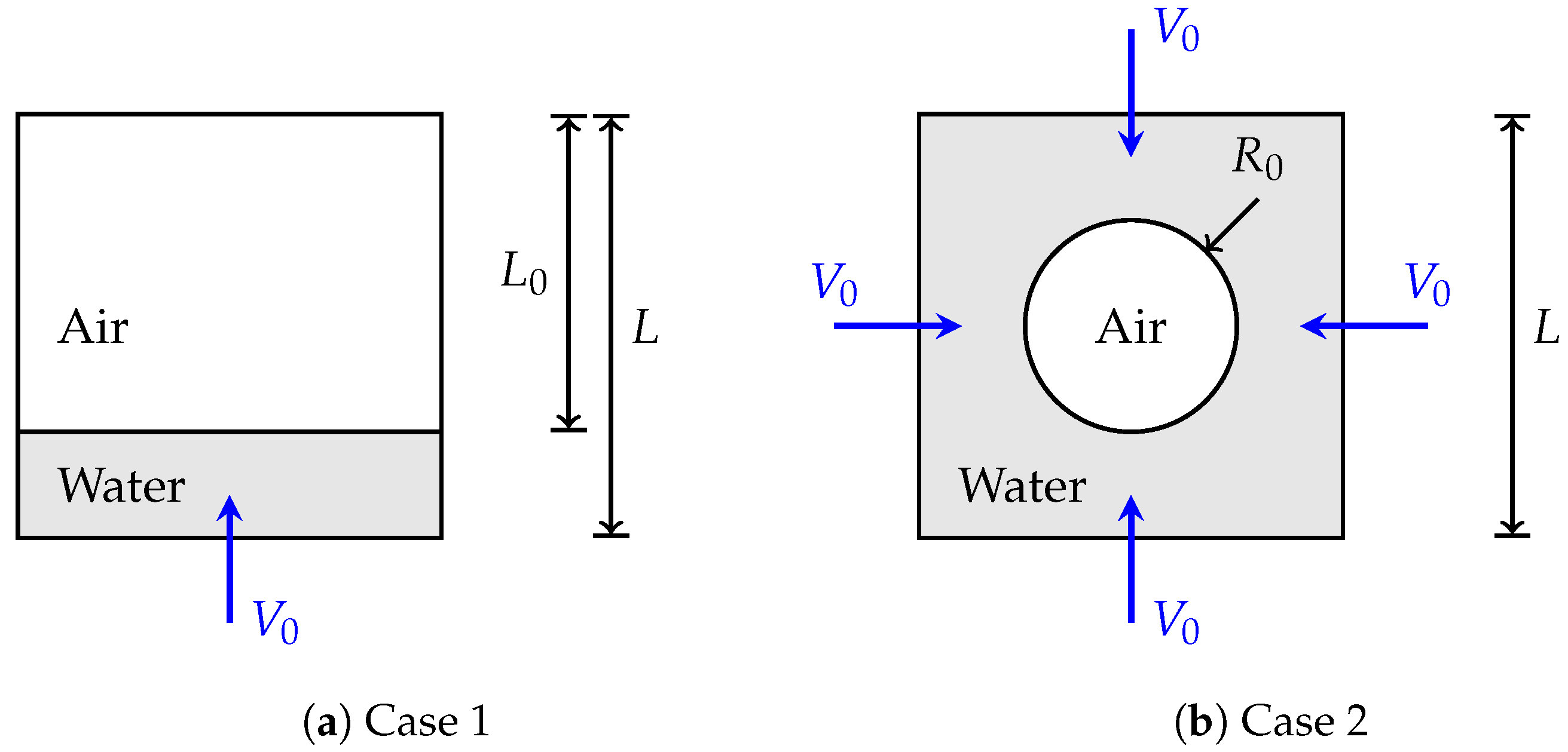
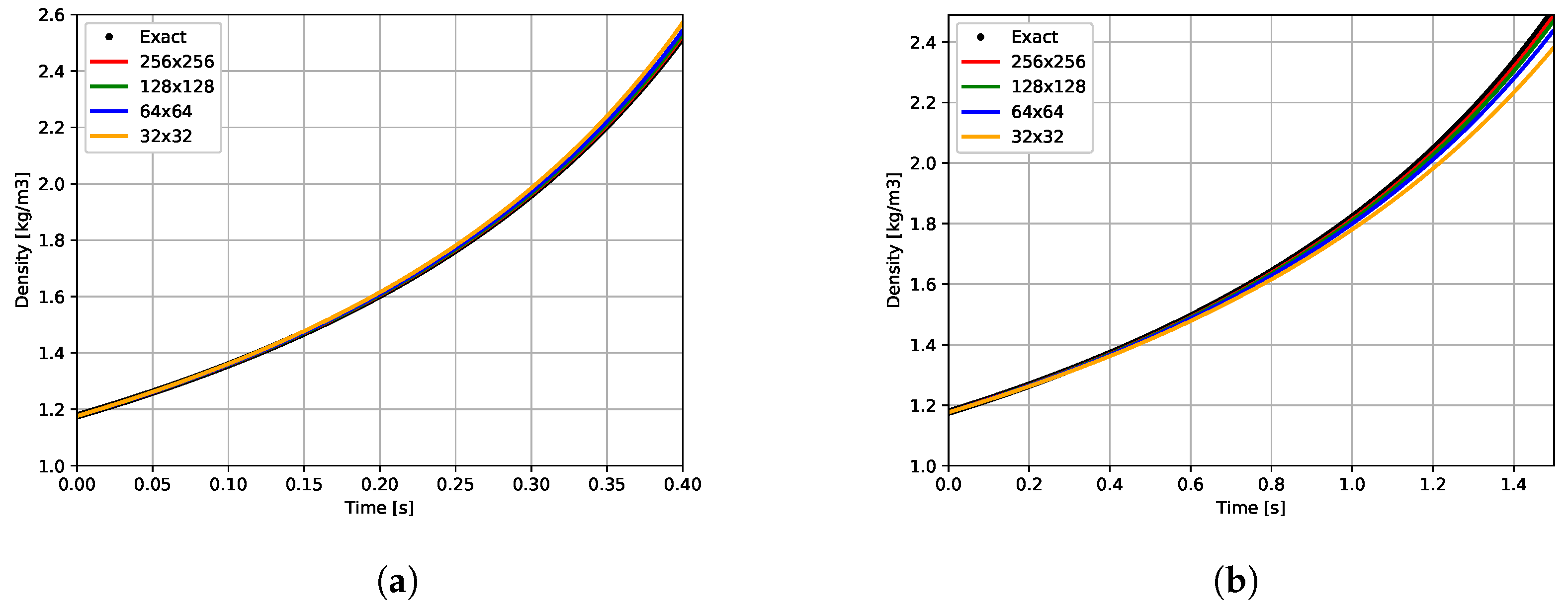
4.2. Isothermal Case for a Viscous Flow without Capillary Effects

In order to validate the compressible two-phase model presented in the previous section, two academic test cases are studied [3] in the context of isothermal and viscous flows. The purpose is to check the accuracy of the compressible model in a simple isothermal two-phase case by comparing the numerical density and pressure fields with the analytical solutions. The relative error is then estimated for various meshes and the convergence order can be extracted. In both cases, the thermophysical characteristics of the two fluids are given in Table 1. The two configurations are quite similar and are presented in Figure 4. In a square cavity of side length L = 0.1 m, air is compressed by a water injection at a constant mass flow rate. The initial air density is ρ 0 . As the analytical solutions to these problems are based on a quasi static evolution hypothesis, the velocity V 0 is chosen to be very low. In configuration (Figure 4a), air initially spans a length L 0 and the water injection velocity is V 0 = 0.1 m/s. The mass of air is constant and its volume will vary over time with the volume of water injected according to the following law:
ρ ( t ) = ρ 0 1 V 0 t L 0 1
In the second case (Figure 4b), an air bubble of initial radius R 0 = 30 mm is compressed by injecting water from all the sides of the square cavity, with V 0 = 2.5 × 10 3 m/s. The theoretical equation for density evolution over time is
ρ ( t ) = ρ 0 1 4 V 0 L t π R 0 2 1
The analytical pressure field p is obtained from the analytical density using the ideal gas model, p ( t ) = ρ ( t ) r T 0 , with T 0 = 300 K as the reference temperature.
In the following, the cases are simulated on four Cartesian grid meshes composed of 32 2 , 64 2 , 128 2 , and 256 2 control volumes, with a constant time step Δ t = 10 4 s and a residual of ε = 10 9 for the iterative solver. The averaged values of the solved density and pressure are used for the gas phase and compared to the analytical solutions in (15) and (16).
Figure 5 presents the density evolution over time. The final time is chosen such that the final density value (or the gas volume) is about twice (half) the initial one. Before discussions about the convergence study of the simulations, it should be noted that all quantities of interest (density and pressure in the air) converge well, for all times, using the referenced solution. The convergence with the number of control volumes is by upper values in case 1 and by lower values in case 2.
Errors in the density and pressure fields, estimated with an L1 relative norm, are presented in Table 2 for both cases. Regarding the relative errors, a Richardson extrapolation is also used on the three finest meshes to find the asymptotic solutions at the final times. A first-order 1 convergence towards the asymptotic values is obtained again.
Note that the convergence orders of pressure and density differ slightly since the errors use quantities at the end of the time step. Density is obtained through step 1 in the global algorithm presented in Section 3, while the pressure field comes from the resolution of the momentum and mass conservation equations (Equations (12a) and (12b)). In case the fields are synchronised before the error computation, the order is strictly the same.

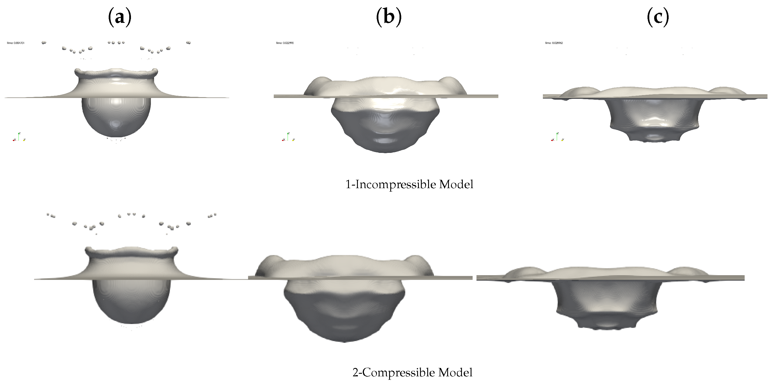
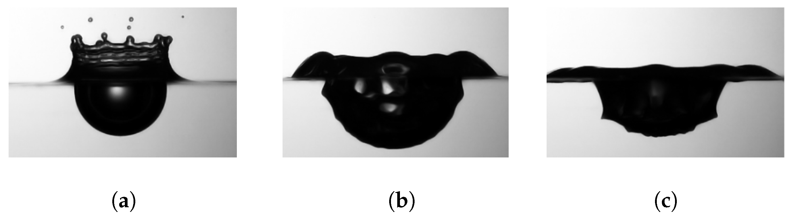
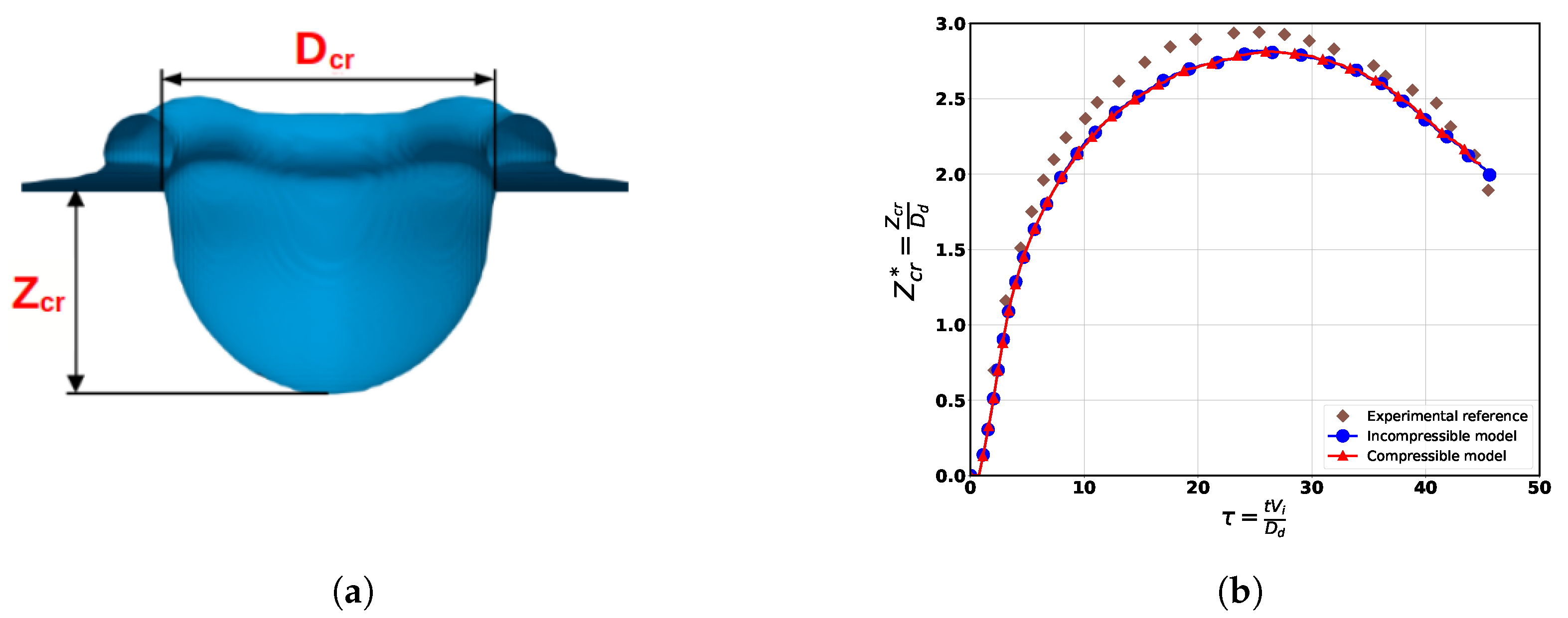
4.3. Isothermal Case for a Viscous Flow with Capillary Effects: Drop Impact on Viscous Liquid Film

As a continuation of the test cases already presented, the drop impact on the viscous liquid film case is set up here. The main aim is to check the ability of our compressible formulation to simulate two-phase flows with large density and viscosity ratios and strong interface deformation. Here, the Mach number is around 0.007 and the flow configuration is almost incompressible. Following the simulations in [23], we consider a drop of water of diameter D = 2.8 × 10 3 m , perfectly circular, with coordinates ( 0 , 0 , 5.15 D ) , placed into a rectangular domain of dimensions L x = 10 D , L y = 10 D , and L z = 20 D . The water surface is initialised at y = 4.5D. The boundary conditions of the domain are non-slip on all faces and homogeneous Neumann on the top. The time step is adaptive, and the CFL is 0.3 . The simulations were carried out with the residual ϵ = 10 5 of BiCGSTAB(2) solver, both with the compressible formulation and with the incompressible scheme.
The results obtained from the compressible and incompressible models are compared with the experimental results shown in Figure 6. Figure 7 shows time snapshots captured at 5, 25, 45, and 65 milliseconds after droplet impact. Initially, as inertia dominates the capillary forces, the drop penetrates the water film and induces the formation of a crater (see Figure 8a) and a rising corona, which later induces a secondary ejection of droplets. After reaching the maximum depth, the crater begins to retract over time due to capillary forces. Finally, compressible and incompressible solvers give identical results that are in agreement with the experiment results (see Figure 6). In addition, in Figure 8b, we can see an equivalence between the compressible model and the incompressible model on the evolution of the crater, in which a good agreement is observed between the numerical results and the experimental measurements. We are dealing with the case where the compressible model degenerates into an incompressible model. We then conclude that our compressible scheme is capable of handling two-phase flows with large interface deformations in incompressible limit of the flow motion.

5. Conclusions

In this work, we introduce a compressible formulation integrated with an original monolithic solver to address two- and three-dimensional compressible interfacial flows, showcasing a concrete progression in computational fluid dynamics. Our developed scheme stands as a notable advancement, providing a dependable and flexible toolkit for accurately and stably simulating diverse fluid flow scenarios, spanning from incompressible to compressible and encompassing both single-phase and two-phase situations with or without capillary effects. Future works will be devoted to the extension of this solver to the validation of the presented model in the case of a droplet splashing into a pool or air bubbles [24,25] or a spray of drops and the interaction between shock/rarefaction waves and fluid/fluid interfaces.

Author Contributions

Conceptualization, S.E.O., S.V. and B.T.; Methodology, S.E.O.; Software, S.V. and B.T.; Validation, S.E.O., S.F. and B.T.; Formal analysis, S.E.O. and S.F.; Investigation, S.E.O., S.V., V.L.C. and A.C.; Writing—original draft, S.E.O.; Writing—review & editing, S.E.O., S.V., V.L.C., B.T. and A.C.; Visualization, S.E.O. and S.F.; Supervision, S.V. All authors have read and agreed to the published version of the manuscript.

Funding

This research received no external funding.

Data Availability Statement

Data are contained within the article.

Acknowledgments

We are grateful for access to the computational facilities of the French CINES (National computing center for higher education) and TGCC granted by GENCI, France, under project number A0112b06115. We thank the technical and administrative teams of these supercomputer centers and agencies for their kind and efficient help. All authors have read and approved the final version of manuscript to be published.

Conflicts of Interest

The authors declare no conflicts of interest.

References

  1. Yoon, S.Y.; Yabe, T. The unified simulation for incompressible and compressible flow by the predictor-corrector scheme based on the CIP method. Comput. Phys. Commun. 1999, 119, 149–158. [Google Scholar] [CrossRef]
  2. Kwatra, N.; Su, J.; Grétarsson, J.T.; Fedkiw, R. A method for avoiding the acoustic time step restriction in compressible flow. J. Comput. Phys. 2009, 228, 4146–4161. [Google Scholar] [CrossRef]
  3. Caltagirone, J.P.; Vincent, S.; Caruyer, C. A multiphase compressible model for the simulation of multiphase flows. Comput. Fluids 2011, 50, 24–34. [Google Scholar] [CrossRef]
  4. Shyue, K.M.; Xiao, F. An Eulerian interface sharpening algorithm for compressible two-phase flow: The algebraic THINC approach. J. Comput. Phys. 2014, 268, 326–354. [Google Scholar] [CrossRef]
  5. Nourgaliev, R.; Luo, H.; Weston, B.; Anderson, A.; Schofield, S.; Dunn, T.; Delplanque, J.P. Fully-implicit orthogonal reconstructed Discontinuous Galerkin method for fluid dynamics with phase change. J. Comput. Phys. 2016, 305, 964–996. [Google Scholar] [CrossRef]
  6. Urbano, A.; Bibal, M.; Tanguy, S. A semi implicit compressible solver for two-phase flows of real fluids. J. Comput. Phys. 2022, 456, 111034. [Google Scholar] [CrossRef]
  7. Fuster, D.; Popinet, S. An all-Mach method for the simulation of bubble dynamics problems in the presence of surface tension. J. Comput. Phys. 2018, 374, 752–768. [Google Scholar] [CrossRef]
  8. Saade, Y.; Lohse, D.; Fuster, D. A multigrid solver for the coupled pressure-temperature equations in an all-Mach solver with VoF. J. Comput. Phys. 2023, 476, 111865. [Google Scholar] [CrossRef]
  9. El Ouafa, M.; Vincent, S.; Le Chenadec, V. Navier-stokes solvers for incompressible single- and two-phase flows. Commun. Comput. Phys. 2021, 29, 1213–1245. [Google Scholar] [CrossRef]
  10. El Ouafa, M.; Vincent, S.; Le Chenadec, V. Monolithic solvers for incompressible two-phase flows at large density and viscosity ratios. Fluids 2021, 6, 23. [Google Scholar] [CrossRef]
  11. El Ouafa, S.; Vincent, S.; Le Chenadec, V.; Trouette, B. Fully-coupled parallel solver for the simulation of two-phase incompressible flows. Comput. Fluids 2023, 265, 105995. [Google Scholar] [CrossRef]
  12. El Ouafa, M. Développement d’un Solveur Tout-Couplé Parallèle 3D Pour la Simulation des Écoulements Diphasiques Incompressibles à Forts Rapports de Viscosités et de Masses Volumiques. Ph.D. Thesis, Université Gustave Eiffel, Champs-sur-Marne, France, 2022. [Google Scholar]
  13. Abgrall, R.; Saurel, R. Discrete equations for physical and numerical compressible multiphase mixtures. J. Comput. Phys. 2003, 186, 361–396. [Google Scholar] [CrossRef]
  14. Saurel, R.; Abgrall, R. A Multiphase Godunov Method for Compressible Multifluid and Multiphase Flows. J. Comput. Phys. 1999, 150, 425–467. [Google Scholar] [CrossRef]
  15. Drui, F.; Larat, A.; Le Chenadec, V.; Kokh, S.; Massot, M. A hierarchy of two-fluid models with specific numerical methods for the simulation of bubbly flows/acoustic interactions. In Proceedings of the APS Division of Fluid Dynamics Meeting Abstracts, APS Meeting Abstracts, San Francisco, CA, USA, 23–25 November 2014; p. R33.003. [Google Scholar]
  16. Brackbill, J.U.; Kothe, D.B.; Zemach, C. A continuum method for modeling surface tension. J. Comput. Phys. 1992, 100, 335–354. [Google Scholar] [CrossRef]
  17. Le Métayer, O.; Saurel, R. The Noble-Abel stiffened-gas equation of state. Phys. Fluids 2016, 28, 046102. [Google Scholar] [CrossRef]
  18. Gottlieb, S.; Shu, C.W.; Tadmor, E. Strong Stability-Preserving High-Order Time Discretization Methods. SIAM Rev. 2001, 43, 89–112. [Google Scholar] [CrossRef]
  19. Nangia, N.; Griffith, B.E.; Patankar, N.A.; Bhalla, A.P.S. A robust incompressible Navier-Stokes solver for high density ratio multiphase flows. J. Comput. Phys. 2019, 390, 548–594. [Google Scholar] [CrossRef]
  20. Weymouth, G.D.; Yue, D.K.P. Conservative volume-of-fluid method for free-surface simulations on cartesian-grids. J. Comput. Phys. 2010, 229, 2853–2865. [Google Scholar] [CrossRef]
  21. Dongarra, J.J.; Duff, I.S.; Sorensen, D.C.; Van der Vorst, H.A. Numerical Linear Algebra for High Performance Computers; Society for Industrial and Applied Mathematics: Philadelphia, PA, USA, 1998. [Google Scholar]
  22. Sod, G.A. A survey of several finite difference methods for systems of nonlinear hyperbolic conservation laws. J. Comput. Phys. 1978, 27, 1–31. [Google Scholar] [CrossRef]
  23. Bisighini, A.; Cossali, G.E.; Tropea, C.; Roisman, I.V. Crater evolution after the impact of a drop onto a semi-infinite liquid target. Phys. Rev. E 2010, 82, 036319. [Google Scholar] [CrossRef]
  24. Zheng, W.; Zhu, B.; Kim, B.; Fedkiw, R. A new incompressibility discretization for a hybrid particle MAC grid representation with surface tension. J. Comput. Phys. 2015, 280, 96–142. [Google Scholar] [CrossRef]
  25. Lentine, M.; Cong, M.; Patkar, S.; Fedkiw, R. Simulating Free Surface Flow with Very Large Time Steps. In Proceedings of the Eurographics/ACM SIGGRAPH Symposium on Computer Animation, Lausanne, Switzerland, 29–31 July 2012; Lee, J., Kry, P., Eds.; The Eurographics Association: Eindhoven, The Netherlands, 2012. [Google Scholar] [CrossRef]
Figure 1. Sod’s shock tube problem: The different colored lines represent the solutions on a 1000-point grid at different times, as indicated by the legend. From the left to the right plot, we display density and pressure along the horizontal axis.
Fluids 09 00090 g001
Figure 2. Sod’s shock tube problem: Comparison of the numerical solution on different grids (using total energy) against the exact solution. The solutions are compared at a physical time of 0.1 s and in a line along the horizontal axis. (a) p. (b) ρ . (c) v . (d) u.
Fluids 09 00090 g002
Figure 3. Sod’s shock tube problem: Comparison of the numerical solution on a 1000-point grid (using total and thermal energy) against the exact solution. The solutions are compared at a physical time of 0.1 s and in a line along the horizontal axis. (a) p. (b) ρ . (c) v . (d) u.
Fluids 09 00090 g003
Figure 4. (a) Water injection in a closed cavity initially full of air. (b) Compression of an air bubble by water injection.
Fluids 09 00090 g004
Figure 5. Density over time for both cases and different grids. Final time is chosen such as that final density is twice initial one. (a) Case 1. (b) Case 2.
Fluids 09 00090 g005
Figure 6. Experimental images [23] of the crater formation inside a deep pool and the rising crown above the liquid surface. (a) is 4.3 ms. (b) is 22.6 ms. (c) is 28.7 ms.
Fluids 09 00090 g006
Figure 7. Simulation of drop impact into a deep pool using different schemes with a resolution of 32 cells per drop diameter. Presentation of the VOF interface ( C = 0.5 isosurface) at three different times: 4.3 ms, 22.6 ms, and 28.7 ms. The simulation with a resolution of 32 cells per drop diameter was carried out on 512 processors of the TGCC IRENE Rome HPC cluster. (a) is 4.3 ms. (b) is 22.6 ms. (c) is 28.7 ms.
Fluids 09 00090 g007
Figure 8. Evolution of the dimensionless crater depth Z c r * as a function of dimensionless time τ for the studied schemes. The numerical results are compared to the experimental measurement in [23]. (a) Definition of the maximum crater depth. (b) Compressible vs. incompressible model using 32 cells per drop diameter.
Fluids 09 00090 g008
Table 1. The physical properties of air (initial) and water used in the computations. Here, water is considered to have a constant density, whereas air is treated as a compressible fluid with an ideal gas law that couples pressure and density. The surface tension between to two phases is neglected.
AirWater
Density ρ (kg · m 3 ) 1.1768292 1000
Viscosity μ (Pa · s) 1.85 × 10 5 1 × 10 3
Compressibility χ T ( Pa 1 ) 9.8692322 × 10 6 0.44 × 10 9
Specific gas constant r (J · K/kg)287
Table 2. Convergence study for both case. Relative error in L 1 norm is computed from analytical relations Equations (15) and (16).
Case 1
Mesh ρ Error L 1 orderpError L 1 order
32 × 32 2.5712.172 × 10−2 2.217 × 1052.114 × 10−2
64 × 64 2.5441.093 × 10−20.982.194 × 1051.034 × 10−21.03
128 × 128 2.5315.580 × 10−30.972.182 × 1054.980 × 10−31.05
256 × 256 2.5242.840 × 10−30.972.176 × 1052.240 × 10−31.15
Extrapolation2.5173.730 × 10−40.972.170 × 1051.200 × 10−30.97
Case 2
Mesh ρ Error L 1 orderpError L 1 order
32 × 32 2.3834.784 × 10−2 2.123 × 1051.652 × 10−2
64 × 64 2.4412.482 × 10−20.942.149 × 1054.310 × 10−30.93
128 × 128 2.4741.137 × 10−21.122.182 × 1054.980 × 10−31.00
256 × 256 2.4905.210 × 10−31.122.188 × 1052.030 × 10−31.08
Extrapolation2.5031.630 × 10−51.122.189 × 1051.640 × 10−31.04
Disclaimer/Publisher’s Note: The statements, opinions and data contained in all publications are solely those of the individual author(s) and contributor(s) and not of MDPI and/or the editor(s). MDPI and/or the editor(s) disclaim responsibility for any injury to people or property resulting from any ideas, methods, instructions or products referred to in the content.

