Unsteady Subsonic/Supersonic Flow Simulations in 3D Unstructured Grids over an Acoustic Cavity

Abstract

In this study, the unsteady Reynolds-averaged Navier–Stokes (URANS) equations are employed in conjunction with the Menter Shear Stress Transport (SST)-Scale-Adaptive Simulation (SAS) turbulence model in compressible flow, with an unstructured mesh and complex geometry. While other scale-resolving approaches in space and time, such as direct numerical simulation (DNS) and large-eddy simulation (LES), supply more comprehensive information about the turbulent energy spectrum of the fluctuating component of the flow, they imply computationally intensive situations, usually performed over structured meshes and relatively simple geometries. In contrast, the SAS approach is designed according to “physically” prescribed length scales of the flow. More precisely, it operates by locally comparing the length scale of the modeled turbulence to the von Karman length scale (which depends on the local first- and second fluid velocity derivatives). This length-scale ratio allows the flow to dynamically adjust the local eddy viscosity in order to better capture the large-scale motions (LSMs) in unsteady regions of URANS simulations. While SAS may be constrained to model only low flow frequencies or wavenumbers (i.e., LSM), its versatility and low computational cost make it attractive for obtaining a quick first insight of the flow physics, particularly in those situations dominated by strong flow unsteadiness. The selected numerical application is the well-known M219 three-dimensional rectangular acoustic cavity from the literature at two different free-stream Mach numbers, $M_{\infty }$ (0.85 and 1.35) and a length-to-depth ratio of 5:1. Thus, we consider the “deep configuration” in experiments by Henshaw. The SST-SAS model demonstrates a satisfactory compromise between simplicity, accuracy, and flow physics description.

1. Introduction

Computational fluid dynamics (CFD) has experienced a notable growth in the last few decades. Nowadays, most engineering designs and technical projects rely on computational predictions before making critical design decisions. Additionally, CFD may also be employed in order to gain important insight into the flow physics before performing an expensive experiment, particularly in the aerospace industry, as recently reviewed by [1]. The workhorse in industrial flow simulations over complex geometries has been the Reynolds-averaged Navier–Stokes (NS) equations (RANS), obtained by time-averaging the full Navier–Stokes equations [2]. These equations demand a closure to compute the Reynolds stresses arising from the convective terms of the NS equations after applying the time-averaging process. Unfortunately, the RANS approach exhibits a deficient performance in massively separated flows or flows with inherently unsteady behavior [3] and in highly accelerated flows [4]. Recently, significant attention has been paid to relatively low-cost, scale-resolving, time-dependent computations of complex flows for industrial applications, e.g., geometries with moving parts, wing flutter, noise prediction, etc. In comparison with the high computational resources demanded by direct numerical or large eddy simulations (DNS/LES) [5], low-cost scale-resolving approaches can provide the best tradeoff between unsteady simulations and unstructured meshes. Particularly, the unsteady Reynolds-averaged Navier–Stokes (URANS) methodology has become quite popular, due to its success in predicting the most energetic modes or coherent structures. However, URANS has frequently been accused of inaccurately representing the correct spectrum of turbulent scales, even if the numerical grid and the time step are of sufficient resolution. In this study, the URANS equations for compressible flows are solved in conjunction with the Menter SST turbulence model and the scale-resolving SAS model (Scale-Adaptive Simulation) by Menter and Egorov [6,7,8]. The adaptive simulation concept allows more details of the flow to be captured, or more turbulent structures. Furthermore, the most significant advantage of the SAS approach over existing DES/LES methods is that the model is developed independent of the grid spacing. The SAS approach introduced by Menter and Egorov [6,7,8] is based on the use of the second derivative of the velocity, which is highly active on short scales. As a consequence, this corresponds to an improvement over the original DES (detached-eddy simulation) model by Spalart et al. [9], which strongly depends on the grid spacing. More recently, a simple modification to the original DES approach (i.e., the delayed DES or DDES) was introduced by Spalart et al. [10] to remedy the grid-induced separation problem of the original DES version based on the shear stress transport formulation (SST) by Menter and Kuntz [11].

Since the testbed for evaluating the Menter SST-SAS model in unstructured meshes is a turbulent cavity in the present study, the most relevant investigation on this topic is discussed hereafter. Comprehensive literature review studies on the physics, numerical modeling, and controlling oscillations in the flow past a cavity have been performed by [12,13] for low- and high-speed incoming flows. In [14], the acoustic influence of front and aft wall modifications for the M219 cavity [15] was analyzed at a free-stream Mach number of 0.85. They used the commercial SIMULIA PowerFlow flow solver, which is based on the lattice Boltzmann method. Seker et al. [14] concluded that aft wall alterations were more efficient in reducing noise. Li et al. [16] performed numerical simulations over a supersonic cavity (Mach 1.5) via a nonlinear acoustic solver (NLAS) to evaluate the near-field cavity noise. They also considered a slanted wall as a passive control technique, achieving a noise reduction of approximately 5 dB with respect to the baseline case.

To our knowledge, most of the numerical fluid dynamics applications of the SAS turbulence model as scale-resolving simulations (SRSs) have been performed in incompressible flows and over structured meshes in relatively simple geometries [17,18,19,20]; whereas, only a few studies have focused on unstructured meshes [21,22,23]. With the purpose of filling that research gap, the Menter SST-SAS model is tested in complex geometries via unstructured grids for the subsonic–supersonic flow regime, then validated with experimental data for the M219 acoustic cavity [15]. The FLITE3D flow solver [24] is applied in the present study, which is based on a finite volume approach with stabilization and discontinuity-capturing features.

2. Governing Equations

The three-dimensional unsteady compressible Navier–Stokes equations are expressed over a volumetric domain $\Omega \subset {\Re }^3$ confined by a surface $\Gamma$ and in integral form as follows:

$${\int }_{\Omega }\frac{\partial U}{\partial t}d\Omega +{\int }_{\Gamma }{F}_j{n}_{j}d\Gamma ={\int }_{\Gamma }{G}_j{n}_{j}d\Gamma ,$$

(1)

where $\overrightarrow{n}=(n_1,n_2,n_3)$ is the unit normal vector to $\Gamma$. Furthermore, the unknown vector of conservative variables is defined as

$$U=\left[\begin{array}{c}\rho \\ \rho u_1\\ \rho u_2\\ \rho u_3\\ \rho ϵ\end{array}\right],$$

(2)

where $\rho$ is the fluid density, $u_i$ denotes the ith component of the velocity vector ($u_1,u_2,u_3$), and $ϵ$ is the specific total energy. The inviscid and viscous flux vectors are expressed as

$$F_j=\left[\begin{array}{c}\rho u_j\\ \rho u_1{u}_j+p{\delta }_{1j}\\ \rho u_2{u}_j+p{\delta }_{2j}\\ \rho u_3{u}_j+p{\delta }_{3j}\\ u_j(\rho ϵ+p)\end{array}\right]G_j=\left[\begin{array}{c}0\\ {\tau }_{1j}\\ {\tau }_{2j}\\ {\tau }_{3j}\\ u_k{\tau }_{kj}-q_j\end{array}\right],$$

(3)

respectively. The quantity

$${\tau }_{ij}=-\frac{2}{3}\mu \frac{\partial u_k}{\partial x_k}{\delta }_{ij}+\mu \left(\frac{\partial u_i}{\partial x_j}+\frac{\partial u_j}{\partial x_i}\right)$$

(4)

is the deviatoric stress tensor, where $\mu$ is the dynamic viscosity. The quantity $q_j=-k\partial T/\partial x_j$ is the heat flux, where k is the thermal conductivity and T is the absolute temperature. The viscosity varies with temperature according to Sutherland’s law and the molecular Prandtl number is assumed to be constant and equal to 0.72. In addition, the medium is assumed to be calorically perfect.

3. Solution Procedure

In this section, numerical strategies for unstructured mesh generation and spatial/time discretization are explained and discussed.

3.1. Hybrid Unstructured Mesh Generation

The computational domain is represented by an unstructured hybrid mesh for viscous problems [2]. The process of mesh generation begins with the discretization of the domain boundary into a set of triangular or quadrilateral meshes that satisfy a mesh control function specified by the user [25]. Additionally, the distribution of the mesh parameters [26], such as spacing, stretching, and direction of stretching, are described by a background mesh as well as point, line, and planar sources. For viscous flows, the boundary layers are generated using the advancing layer method [27] and the rest of the computational domain is filled with tetrahedral elements using a Delaunay incremental Bowyer–Watson point insertion [28]. Hybrid unstructured meshes are constructed by merging certain elements of this tetrahedral mesh in the boundary layers.

3.2. Spatial Discretization

The discretization of the governing equations can be performed in a number of different ways. A computationally efficient approach is implemented, consisting of a cell vertex finite volume method. This involves the identification of a dual mesh, with the medial dual being constructed as an assembly of triangular facets, ${\Gamma }_I^K$, where each facet is formed by connecting edge midpoints, element centroids, and face centroids in the basic mesh in such a way that only one node is contained within each dual mesh cell. Hence, the dual mesh cells form the control volumes for the finite volume process. When hybrid meshes are employed, the method for constructing the median dual has to be modified in order to ensure that no node lies outside its corresponding control volume. To perform the numerical integration of the fluxes, a set of coefficients is calculated for each edge using the dual mesh segment associated with the edge. The values of the internal edge coefficients, $C_j^{IJ}$, and the boundary edge coefficients, $D_j^{IJ}$, are defined as follows:

$$C_j^{IJ}=\sum _{K\in {\Gamma }_{IJ}}{A}_{{\Gamma }_I^K}{n}_j^{{\Gamma }_I^K},D_j^{IJ}=\sum _{K\in {\Gamma }_{IJ}^B}{A}_{{\Gamma }_I^K}{n}_j^{{\Gamma }_I^K},$$

(5)

where $A_{{\Gamma }_I^K}$ is the area of facet ${\Gamma }_I^K$, $n_j^{{\Gamma }_I^K}$ is the outward unit normal vector of the facet, ${\Gamma }_{IJ}^B$ is the set of dual mesh faces on the computational boundary touching the edge between nodes I and J, and $n_j^{{\Gamma }_I^K}$ denotes the facet normal to the outward direction of the computational domain. The numerical integration of the fluxes over the dual mesh segment associated with an edge is carried out by assuming that the flux is constant and equal to its approximated value at the midpoint of the edge, i.e., a form of midpoint quadrature. The calculation of a surface integral for the inviscid flux over the control volume surface for node I is defined as follows:

$${\int }_{\partial {\Omega }_I}{F}_j{n}_{j}d\mathbf{x}\approx \sum _{J\in {\Lambda }_I}\frac{C_j^{IJ}}{2}\left(F_j^I+F_j^J\right)+\sum _{J\in {\Lambda }_I^B}{D}_j^{IJ}{F}_j^I,$$

(6)

where ${\Lambda }_I$ denotes the set of nodes connected to node I by an edge and ${\Lambda }_I^B$ denotes the set of nodes connected to node I by an edge on the computational boundary. Thus, the last term is non-zero only in a boundary node. A similar formula can be implemented for the viscous fluxes. Such an edge-based data structure has become widely used due to its efficiency in terms of memory and CPU requirements compared to the traditional element-based data structure, in particular in three dimensions.

The resulting discretizations are basically central difference in character. Therefore, the addition of a stabilizing dissipation is required for practical flow simulations. This is achieved by replacing the physical flux function by a consistent numerical flux function, such as the JST flux function [29] or the HLLC solver [30]. Discontinuity capture may be accomplished by the use of an additional harmonic term in regions of high pressure gradients, identified using a pressure switch.

3.3. Time Discretization

The FLITE3D flow solver can simulate both unsteady and steady problems. However, in this investigation an unsteady flow analysis is performed. A three-level, second-order accurate backward difference scheme is utilized in the present investigation:

$$\frac{\partial U_i}{\partial t}{|}_{t=t_n}=\frac{1}{▵t}\left(\frac{3}{2}{U}_i^n-2U_i^{n-1}+\frac{1}{2}{U}_i^{n-2}\right)+\mathcal{O}(▵t^2),$$

(7)

Additionally, the relaxation scheme employed at each physical time step consists of a three-stage Runge–Kutta approach with local time-stepping. The viscous and artificial dissipation terms are only computed once at every time step in order to reduce the computational requirements of the scheme. More details can be found in [31].

4. Turbulence Modeling in RANS

To obtain the compressible RANS equations, the unsteady Equation (1) is time-averaged to smooth the instantaneous turbulent fluctuations in the flow field, while still allowing the capture of the time-dependency on the time scales of interest. In many engineering problems this assumption is valid, but this averaging procedure breaks down if the timescale of the physical phenomena of relevance is similar to that of the turbulence itself. For compressible flows, the density-weighted Favre averaging procedure is mostly employed [31]. The Favre averaging procedure applied to Equation (1) generates the extra convective term

$${\tau }_{ij}^R=-\overline{\rho u_i^{″}{u}_j^{″}},$$

(8)

which is the Favre-averaged Reynolds stress tensor. The most straightforward approach is to associate the unknown Reynolds stresses with the computed mean flow quantities by means of a turbulence model. If the Boussinesq hypothesis is applied, this results in a linear relationship to the mean flow strain tensor through the eddy viscosity ${\mu }_t$ [32]:

$${\tau }_{ij}^R={\mu }_t\left(\frac{\partial u_i}{\partial x_j}+\frac{\partial u_j}{\partial x_i}-\frac{2}{3}\frac{\partial u_k}{\partial x_k}{\delta }_{ij}\right)-\frac{2}{3}\rho k{\delta }_{ij},$$

(9)

where k is the turbulent kinetic energy. The eddy viscosity depends on the velocity and the length scales of the turbulent eddies, i.e., ${\mu }_t\sim k^{1/2}$ℓ, where ℓ is the turbulence length scale. In this paper, a two-transport-equation model is considered in which additional partial differential equations are solved to describe the transport of the eddy viscosity. As a consequence, nonlocal and history effects on ${\mu }_t$ are taken into account. Two-equation turbulence models are complete, because transport equations are solved for both turbulent scales, i.e., the velocity and the length scales. In particular, the $k-\omega$ turbulence model is popular due to its good performance in boundary layer flows subjected to adverse pressure gradients, with eventual separation. The original $k-\omega$ model [32] exhibits a free-stream dependency of $\omega$, which is generally not present in the $k-ϵ$ model. Menter [33] combined the advantages of both models by means of blending functions, that permit the switching from $k-\omega$, close to a wall, to $k-ϵ$, when approaching the edge of a boundary layer. A further improvement [33] was a modification to the eddy viscosity based on the idea of the Johnson–King model, which establishes that the transport of the main turbulent shear stresses is crucial in the simulations of strong adverse-pressure-gradient flows. This new approach was called the Menter Shear Stress Transport model (SST), which was already implemented in FLITE3D for steady-state solutions via the RANS approach [2].

4.1. Scale-Adaptive Simulations (SASs) in Unsteady Flows

In this section, a brief description of the SAS equations is shown. The differential equations are presented in the normalized form. A convenient scaling guarantees a unit order of all variables, which decreases round-off errors of calculations. The reader is referred to Appendix B of Sørensen’s thesis [31] for the scaling and the normalized versions of the momentum and energy equations employed in the present study; however, the normalization symbol * is dropped for simplicity. The corresponding normalized transport equations in the Menter SST model [33] for the turbulent kinetic energy, k, and the specific dissipation rate, $\omega$, in compressible flows read as follows:

$$\underset{\mathrm{transient} \mathrm{term}}{\underbrace{\frac{1}{S{t}_{\infty }}\frac{\partial \left(\rho k\right)}{\partial t}}}+\underset{\mathrm{convection} \mathrm{term}}{\underbrace{\frac{\partial \left(\rho u_{j}k\right)}{\partial x_j}}}=\underset{\mathrm{production} \mathrm{term}}{\underbrace{{\tau }_{ij}\frac{\partial u_j}{\partial x_j}}}-\underset{\mathrm{dissipation} \mathrm{term}}{\underbrace{{\beta }_k\rho \omega k}}+\underset{\mathrm{diffusion} \mathrm{term}}{\underbrace{\frac{1}{R{e}_{\infty }}\frac{\partial }{\partial x_j}\left[\left(\mu +\frac{{\mu }_t}{{\sigma }_k}\right)\frac{\partial k}{\partial x_j}\right]}}$$

(10)

$$\begin{array}{c}\underset{\mathrm{transient} \mathrm{term}}{\underbrace{\frac{1}{S{t}_{\infty }}\frac{\partial \left(\rho \omega \right)}{\partial t}}}+\underset{\mathrm{convection} \mathrm{term}}{\underbrace{\frac{\partial \left(\rho u_j\omega \right)}{\partial x_j}}}=\underset{\mathrm{production} \mathrm{term}}{\underbrace{\alpha \frac{\omega }{k}{\tau }_{ij}\frac{\partial u_j}{\partial x_j}}}-\underset{\mathrm{dissipation} \mathrm{term}}{\underbrace{{\beta }_{\omega }\rho {\omega }^2}}+\underset{\mathrm{diffusion} \mathrm{term}}{\underbrace{\frac{1}{R{e}_{\infty }}\frac{\partial }{\partial x_j}\left[\left(\mu +\frac{{\mu }_t}{{\sigma }_{\omega }}\right)\frac{\partial \omega }{\partial x_j}\right]}}\hfill \\ +\underset{\mathrm{cross-diffusion} \mathrm{term}}{\underbrace{2(1-F_1)\frac{\rho {\sigma }_{\omega 2}}{\omega }\frac{\partial k}{\partial x_j}\frac{\partial \omega }{\partial x_j}}}+Q_{SAS},\hfill \end{array}$$

(11)

where $S{t}_{\infty }=U_{\infty }t/L$ and $R{e}_{\infty }=\rho U_{\infty }L/{\mu }_{\infty }$ are the Strouhal and Reynolds numbers, respectively, $u_j$ represents the Favre-averaged velocity, and ${\mu }_{\infty }$ is the free-stream dynamic viscosity. Furthermore, ${\beta }_k$ = 0.09, ${\beta }_{\omega }$ = 3/40, ${\sigma }_k$ = 2, ${\sigma }_{\omega }$ = 2, $\alpha$ = 5/9, and ${\sigma }_{\omega 2}=0.856$. $F_1$ is a blending function defined as

$$F_1=tanh\left\{\left[min\left(max\left(\frac{\sqrt{k}}{{\beta }_k\omega y},\frac{500\nu }{y^2\omega R{e}_{\infty }}\right),\frac{4\rho {\sigma }_{\omega 2}k}{C{D}_{k\omega }{y}^2}\right)\right]\right\},$$

(12)

and

$$C{D}_{k\omega }=max\left(\frac{2\rho {\sigma }_{\omega 2}}{\omega }\frac{\partial k}{\partial x_j}\frac{\partial \omega }{\partial x_j},{10}^{-10}\right).$$

(13)

Thus, the blending function $F_1$ generates values close to one far from the wall ($k-ϵ$ model) and almost-zero values inside the boundary layer ($k-\omega$ model). More details can be found in [33]. The main features of the Menter SST model can be summarized as follows: (i) the consideration of a cross-diffusion term in the $\omega$ equation; (ii) the implementation of a stress limiter for the maximum value of $\omega$, as well as a production limiter to impede the build-up of turbulence in stagnation zones; and (iii) the application of a blending function to compute the corresponding constants of the $k-ϵ$ and $k-\omega$ models, respectively.

The stress limiter in the Menter SST turbulence model is defined as

$${\mu }_t=\frac{R{e}_{\infty }\rho a_{1}k}{max(a_1\omega ,S{F}_2)},$$

(14)

where $a_1$ = 0.31, $S=\sqrt{2S_{ij}{S}_{ij}}$ is the strain rate, and the normalized function $F_2$ is expressed as

$$F_2=tanh\left\{{\left[max\left(\frac{2\sqrt{k}}{{\beta }_k\omega y},\frac{500\nu }{y^2\omega R{e}_{\infty }}\right)\right]}^2\right\}.$$

(15)

The production limiter consists in taking the minimum of $\left({\tau }_{ij}\frac{\partial u_j}{\partial x_j},10{\beta }_k\rho k\omega \right)$ when solving Equation (10).

The term $Q_{SAS}$ in Equation (11) is the only modification to the SST model to consider the von Karman length scale in the turbulence equation. Hence, the information provided by the von Karman length scale, $L_{\nu K}$, permits the SAS model to dynamically adjust to resolve the large structures in a URANS simulation. This results in LES-like behavior in unsteady regions of the flow field. In addition, the model yields standard RANS capabilities in stable flow regions. The term $Q_{SAS}$ is defined as follows:

$$Q_{SAS}=\rho F_{SAS}max\left\{{\zeta }_2\kappa S^2{\left(\frac{L}{L_{\nu K}}\right)}^2-\frac{2k}{{\sigma }_{\varphi }}max\left[\frac{{|\nabla \omega |}^2}{{\omega }^2},\frac{{|\nabla k|}^2}{k^2}\right],0\right\},$$

(16)

where $F_{SAS}=1.25$, ${\zeta }_2=1.755$, $\kappa =0.41$ (von Karman constant), and ${\sigma }_{\varphi }=2/3$. Furthermore, the corresponding length scales in Equation (16) are

$$L=\frac{\sqrt{k}}{C_{\mu }^{1/4}\omega },$$

(17)

$$L_{\nu K}=max\left\{\frac{\kappa S}{|{\nabla }^{2}u|},C_S\Delta \sqrt{\frac{\kappa {\zeta }_2}{{\beta }_{\omega }/C_{\mu }-\alpha }}\right\},$$

(18)

where $C_S=0.11$ (Smagorinsky constant), $C_{\mu }=0.09$, and $\Delta$ is the cubic root of the control volume size. Note that the term $Q_{SAS}$ in Equation (16) is always positive, and basically depends on the ratio between the length scale of the modeled turbulence, L, to the von Karman length scale, $L_{\nu K}$. Thus, where this ratio (i.e., $L/L_{\nu K}$) is large enough in the computational domain, the term $Q_{SAS}$ becomes larger, making the turbulence viscosity, ${\mu }_t$, smaller. Consequently, the large unsteady structures break up into a turbulent spectrum.

4.2. Discretization of the Turbulent Transport Equations

The turbulence model equations involve the solution of partial differential equations, which are discretized in a similar manner as the governing equations. Nevertheless, to avoid instabilities from the convective terms, a first-order upwind discretization of this term is used, plus an added term to introduce adequate dissipation for stabilization:

$$\begin{array}{cc}\hfill & {\int }_{\partial {\Omega }_I}{u}_{j}tu{n}_{j}d\mathbf{x}\approx \sum _{J\in {\Lambda }_I}\frac{C_j^{IJ}}{2}\left(u_j^{I}t{u}_I+u_j^{J}t{u}_J\right)-\left(C_j^{IJ}\frac{u_j^{J}t{u}^J-u_j^{I}t{u}^I}{t{u}_J-t{u}_I}\right)(t{u}_J-t{u}_I)+\hfill \\ \hfill & \sum _{J\in {\Lambda }_I^B}{D}_j^{IJ}{\mathbf{F}}_j^I,\hfill \end{array}$$

(19)

where tu stands for turbulence unknowns ($\tilde{\nu }$, k, and $\omega$). Furthermore, the volume integrals are calculated using the midpoint rule and the gradients appearing in the model are calculated as follows:

$${\int }_{{\Omega }_I}\frac{\partial u_i}{\partial x_j}d\mathbf{x}={\int }_{\partial {\Omega }_I}{u}_i{n}_{j}d\mathbf{x},$$

(20)

Equation (20) in discrete form reads

$$\frac{\partial u_i}{\partial x_j}{|}^I\approx {\partial }_j^h{u}_i^I\equiv \frac{1}{V_I}\left[\sum _{J\in {\Lambda }_I}\frac{C_j^{IJ}}{2}\left(u_i^I+u_j^J\right)+\sum _{J\in {\Lambda }_I^B}{D}_j^{IJ}{u}_i^I\right],$$

(21)

where $V_I$ is the volume of the control volume, ${\Lambda }_I$ denotes the set of nodes connected to node I by an edge, and ${\Lambda }_I^B$ stands for the set of nodes connected to node I by an edge on the computational boundary. Coefficients $C_j^{IJ}$ and $D_j^{IJ}$ represent the contribution to integrals from internal and boundary edges. Equations (20) and (21) are expressed for the velocity but can be applied to any flow parameter. The second-order diffusion term is calculated using the compact stencil of equation according to eq. (3.38) in [31], where the gradients along the edges are evaluated by means of the compact finite difference scheme.

5. Initial and Boundary Conditions

In all cases, the unsteady solution was started from the steady one. Furthermore, the initial conditions for the first stage (steady solution) were free-stream conditions. The boundary conditions for the flow parameters (i.e., velocity, density, and total energy) were already discussed in [24]. In this section, focus is given to the corresponding boundary conditions of the turbulence variables. Furthermore, the boundary conditions employed in this investigation are classified as solid wall, inflow, outflow, and symmetry.

5.1. Solid Wall Boundary

In the Menter SST model, the turbulent kinetic energy, k, is assigned a zero value at the wall. The specific dissipation rate, $\omega$, does not possess a natural boundary condition at the wall. However, based on the asymptotic solution given by Wilcox [32], the following value for $\omega$ is prescribed according to the implemented normalization:

$${\omega }_o=\frac{6{\nu }_w}{\beta y_w^{2}R{e}_{\infty }},$$

(22)

where ${\nu }_w$ is the laminar kinematic viscosity at the wall, $\beta$ is a constant (=3/40), $y_w$ is the local first off-wall point, and $R{e}_{\infty }$ is the Reynolds number.

5.2. Inflow and Outflow Boundaries

Based on recommendations by [34], the following values for $k_{\infty }$ and ${\omega }_{\infty }$ are adopted in the two-equation turbulence models at these boundaries: $1\times {10}^{-6}$ and 5, respectively.

5.3. Symmetry Boundary

A symmetry condition is defined as a boundary where the velocity component normal to the surface is set to zero and the gradient of any flow parameter in the surface normal direction is set to zero as well. Furthermore, a symmetry condition can also be compared to an inviscid wall (streamline). Hence, the turbulent eddy viscosity is set to zero at this location in the turbulence models. If the configuration of the problem possesses a symmetry plane, this represents a very convenient way to significantly reduce the computational resources required.

6. Results and Discussion

The Menter SST-SAS turbulence model was implemented in the FLITE3D flow solver [24]. The results of the classical M219 acoustic cavity are presented in this section, together with a discussion concerning the application of the models.

M219 Acoustic Cavity

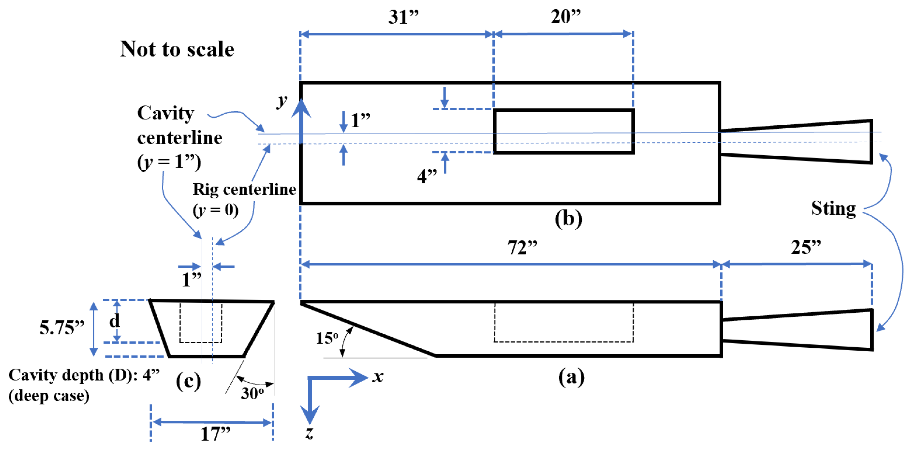
Numerical simulations of flow over a fully 3D subsonic/supersonic rectangular cavity are presented and discussed in this section. The vortex system and flow patterns inside a rectangular three-dimensional acoustic cavity consist of intricate fluid dynamics structures, highly dictated by the incoming flow regime and geometry dimensions. For the purpose of testing the Menter SST-SAS turbulence model, the cavity configuration is selected as the M219 experimental test case of Henshaw [15] for a deep cavity (4 inches) at two different free-stream Mach numbers ($M_{\infty }$ = 0.85 and 1.35). An adapted schematic of the experimental model used in [15] is shown in Figure 1. In [15], ceiling static pressure was measured at the rig centerline ($y=0$) for the deep cavity and off-centerline (i.e., at the cavity centerline, $y=1^{″}$) for the shallow cavity via Kulite transducers. Note that the cavity centerline is displaced by $1^{″}$ with respect to the rig centerline. In the present study, only the measured root mean square (RMS) value of the ceiling static pressure at the rig centerline (y = 0) was employed for numerical validation of the deep cavity (K20 to K29 transducers). 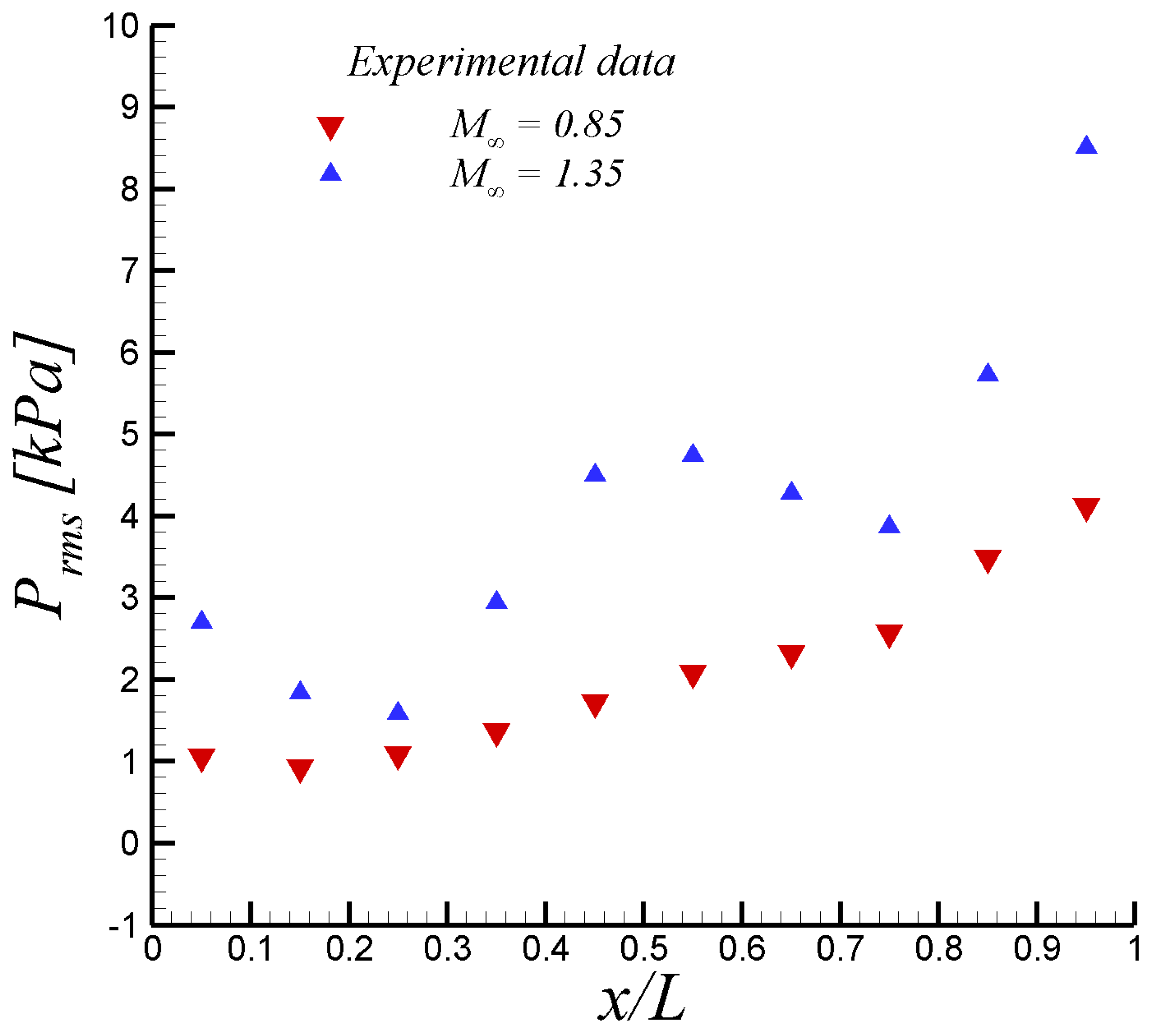Figure 2 depicts the RMS static pressure distribution over the ceiling of the deep empty cavity. It is observed that incoming high-subsonic-Mach-number flow induces a slightly increasing RMS distribution, with a growing factor of approximately four between the last (K29) and first (K20) Kulite transducers. However, the RMS distribution at Mach 1.35 exhibits a wavy trend, with local minima at $x/L\approx$ 0.25 and 0.75, respectively.

The geometry dimensions of the M219 cavity in terms of the depth are $L\times W\times D=5\times 1\times 1$ (length, width, and depth), with a depth, D, of 4 inches. Since the width and depth of the cavity are the same, this configuration create a fully three-dimensional flow pattern. The Reynolds number spans 9.5 × ${10}^6$ to 21 × ${10}^6$, based on the cavity depth. The incoming flat-plate boundary layer is turbulent, with the ratio of the upstream boundary layer thickness to the cavity depth, i.e., $\delta /D$, approximately ranging from 0.1 to 0.25 for Mach numbers of 0.85 and 1.35, respectively. The unstructured hybrid mesh (hereafter fine mesh) is composed of approximately 3.37 million tetrahedral elements, 4472 prisms, and 459 pyramids. This element distribution was determined to be deemed appropriate for the goals of this study and cavity representation based on the initial grid-independent study performed. An initial coarse hybrid mesh was designed and created according to our past experience with steady RANS [2], having approximately 30 to 40% fewer elements than the fine mesh. It is important to mention that when dealing with unsteady simulations or LES-like approaches (scale-resolving simulations) such as the SST-SAS model, it is clear that the outcomes are determined by the numerical approach and grid point distribution utilized. However, performing successive “grid refinements” to achieve absolute grid-independent results would lead to DNS outcomes, which is not consistent with the purpose of assessing turbulence model resilience.

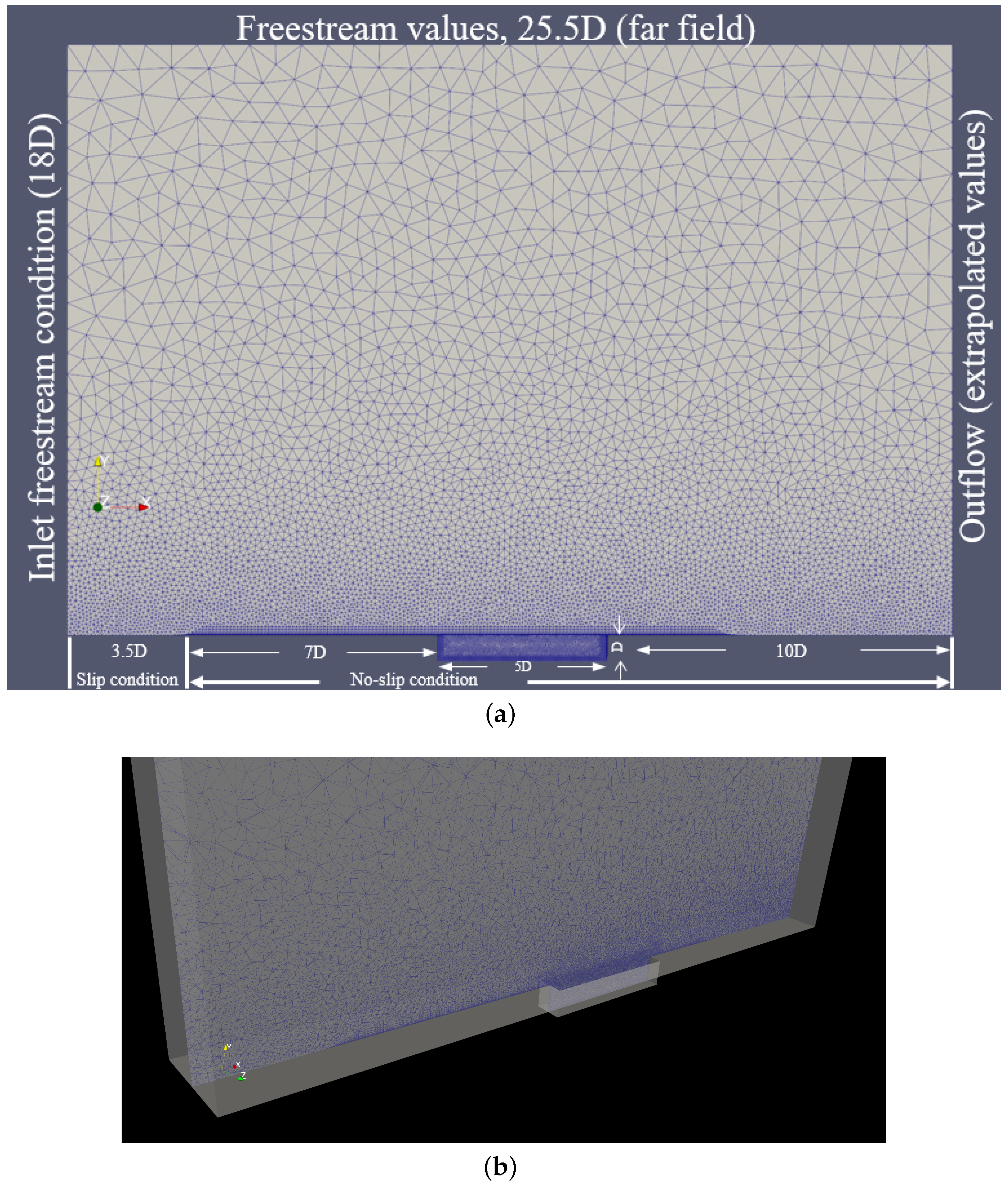
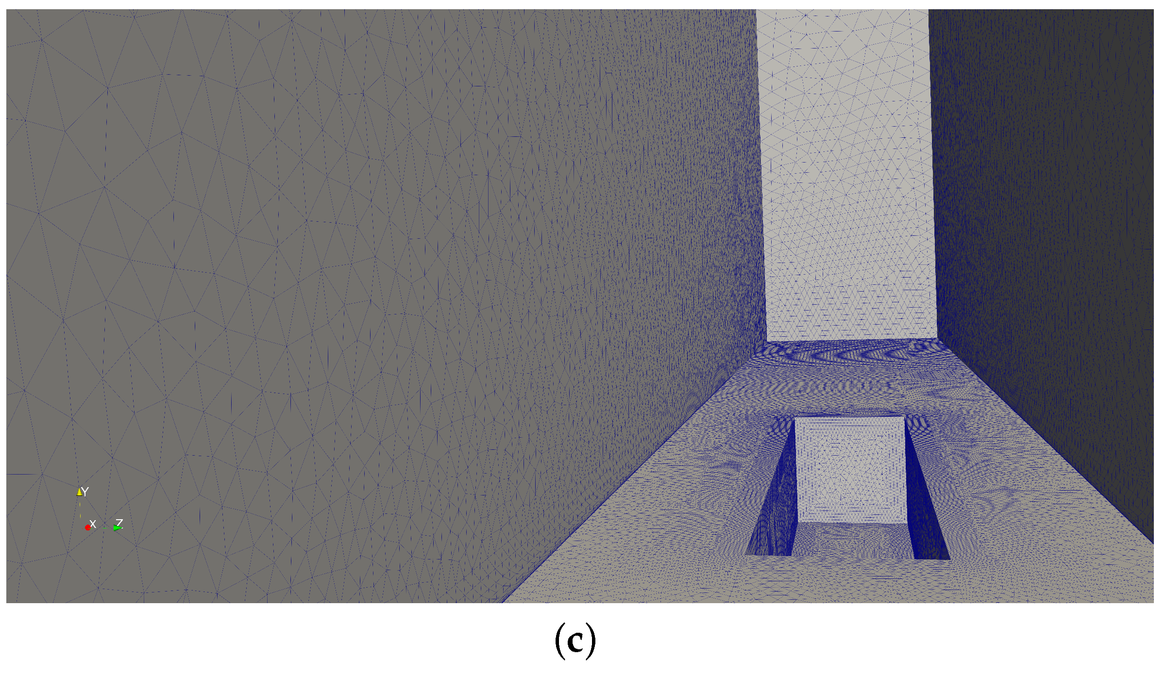
Some views of the computational domain, boundary conditions, and grid system are displayed in Figure 3. A right-side view (flow from left to right) is shown in Figure 3a with the corresponding dimensions in terms of the cavity depth and boundary conditions, which are further described later in the paper. Note that the coordinates y and z represent the vertical and spanwise directions, respectively, in the present study, whereas the opposite was assumed in [15]. Also, note that the origin coordinate system is prescribed at the cavity centerline ($z=0$) in this manuscript. An isometric view of the full computational domain and mesh schematic at the half-plane of the cavity is shown in Figure 3b. Also, an interior cavity view is depicted in Figure 3c. The mesh has 20 viscous layers for efficient boundary layer capturing, with the first off-wall point located at $y/D=2.5\times {10}^{-6}$. The layers, based on prisms to capture the viscous shear layer, are stretched in the wall-normal direction but with the same heights in the streamwise direction of the no-slip surfaces around and inside the cavity. This ensures that the first off-wall point locations are within 0.2 to 0.4 wall or plus units inside the viscous linear layer. Furthermore, the viscous layers (structured mesh) are prescribed in no-slip condition surfaces. It was decided to cluster tetrahedral elements (unstructured mesh) inside the cavity (away from solid surfaces) and above it, based on a high-quality and high-resolution tetrahedral mesh. The total dimensions of the computational domain are as follows: $25.5D\times 18D\times 3D$ along the streamwise, vertical, and spanwise directions, respectively, and in terms of the cavity depth, D. Therefore, the computational domain is tall enough and wide enough to eliminate any influence from the boundary faces on the flow statistics over the cavity. Moreover, the spanwise side walls are treated as symmetry (periodic) planes, the top boundary is a far-field boundary, and all bottom solid surfaces (including the cavity) are considered as adiabatic non-slip walls. Upstream of the cavity edge, a flat-plate with no-slip condition is prescribed (about 7D in length). While a zone with slip condition (and inlet free-stream flow parameters) is set-up upstream of the flat plate (∼3.5D in length). A zero flux condition is prescribed at the outflow plane, where flow parameters are extrapolated from within the domain (see Figure 3a).

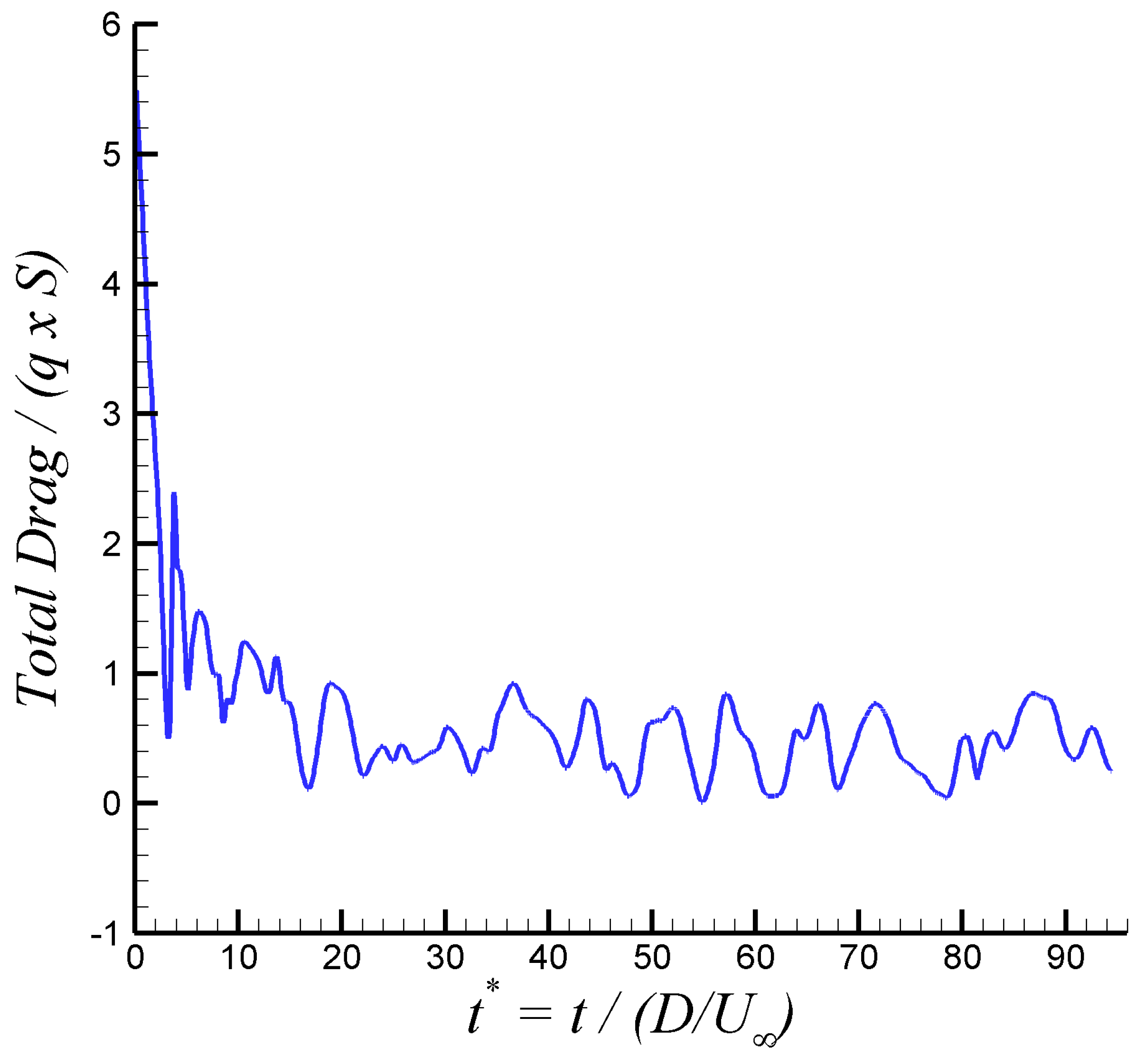
The selected normalized time step is $\Delta t^{*}=\Delta t/(D/U_{\infty })=0.05$, approximately $1.74\times {10}^{-5}$ s at $M_{\infty }$ = 0.85 or $1.3\times {10}^{-5}$ s at $M_{\infty }$ = 1.35. According to Rajkumar et al. [23], the SAS model enables a larger time step size than DES approaches due to its RANS nature. Their physical time steps were about 1.8 to 2.5 smaller than in the present study for a similar cavity configuration via SAS predictions. The time variation of the total drag over the cavity at $M_{\infty }$ = 0.85, normalized by the reference surface and free-stream dynamic pressure, can be observed in Figure 4. Furthermore, the transient stage took approximately 15 non-dimensional time units from the steady solution, as seen in Figure 4. This transient part was discharged for flow statistics computation. The results were sampled, and statistics were computed after the transient stage. All flow parameters and the RMS of pressure were computed via assembled time-averaging, except in the flow visualization analysis where instantaneous flow fields were considered. The numerical data were collected during the last 81 non-dimensional time units, about 1000 flow fields were saved for post-processing analysis. According to [15], the experimental pressure data were sampled at 6000 Hz with a block size of 1024 units. Therefore, the sampling collection for statistical analysis is deemed adequate for the objectives of this study.

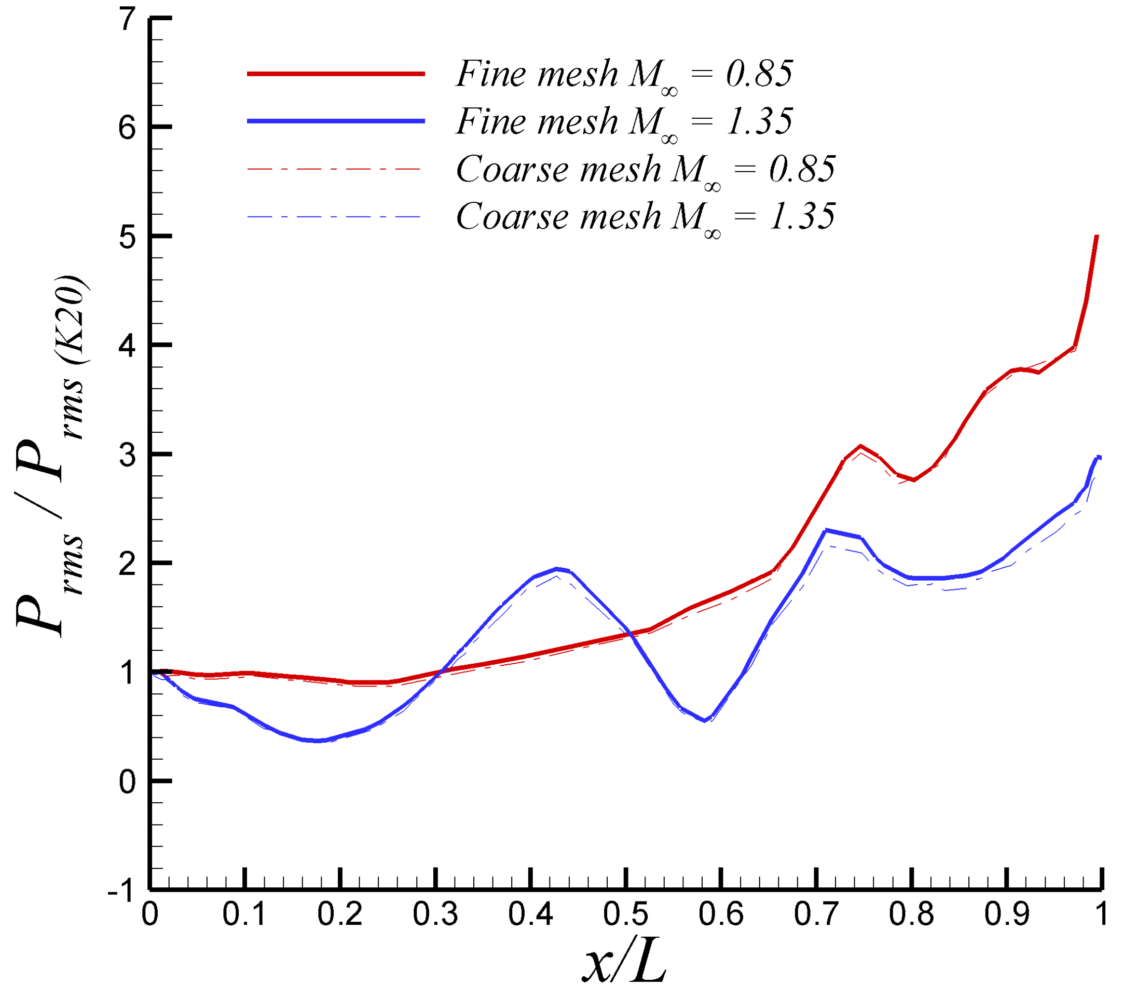
Figure 5 shows the numerical results via the SST-SAS model for the fine and coarse mesh. Overall, predictions from both meshes are very similar, with some discrepancies, particularly for the supersonic case ($M_{\infty }$ = 1.35). However, those differences in numerical values between both meshes were computed as 2% at most, which demonstrates grid-independent outcomes for the fine mesh. Henceforth, numerical results from the SST-SAS model are from the fine mesh. 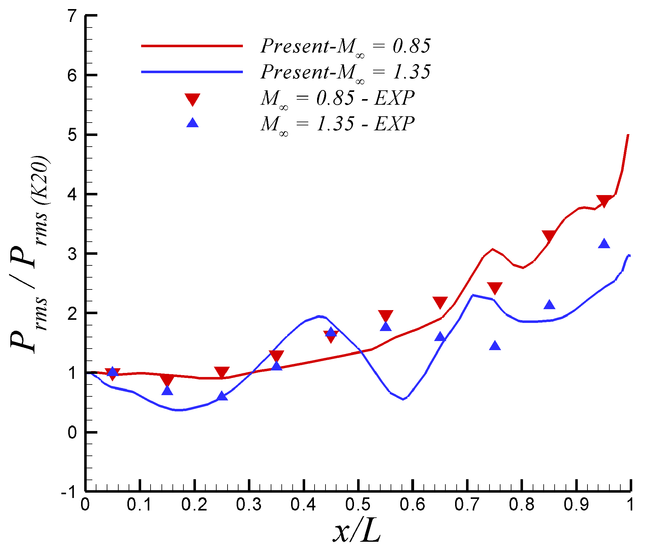Figure 6 depicts the root mean square (RMS) of pressure fluctuations on the cavity ceiling at $z/D$ = −0.25 (rig centerline) and both free-stream Mach numbers. Note that in Figure 6 the values of $P_{rms}$ were normalized by the value at the first transducer (i.e., K20), located 1 inch downstream of the front of the cavity, in experiments by Henshaw [15]. The comparison of the present SST-SAS results at $M_{\infty }$ = 0.85 with the experimental data from [15] is fairly good. The SAS model is able to capture the increasing slope of $P_{rms}$ by the cavity end. On the other hand, the performance of the SAS model in the supersonic regime ($M_{\infty }$ = 1.35) is not as good as in the subsonic case. While the first inflexion point (around $x/L$ = 0.35) is well captured, the second inflexion point in experimental $P_{rms}$ is improperly outlined by the SST-SAS model. This may be attributed to the presence of some important compressibility effect on the cavity flow, which is not taken into account in the SAS approach. The corresponding average discrepancies between the SST-SAS results and the experiments were computed to be approximately $0.13(P_{rms}/P_{rmsK20})$ and $0.26(P_{rms}/P_{rmsK20})$ units at Mach numbers of 0.85 and 1.35, respectively. According to reference [15], the basic accuracy of the system in measuring experimental values of pressure was shown to be ±0.5%. The original SAS model was designed and mostly tested in incompressible and low-Mach-number wall-bounded flow applications [7,8]. Previous work on turbulent coherent structures by [35,36] via two-point correlations (TPCs) and the Lagrangian coherent structure (LCS) approach has revealed a moderate compressibility effect (but not negligible) on the coherent structure dimensions. Specifically, Lagares and Araya [36] stated “coherent structures grow more isotropic proportional to the Mach number, and their inclination angle varies along the streamwise direction”. Therefore, it can be inferred that the SAS turbulence model would be greatly enhanced by the addition of a Mach number dependency of the length scale computation of the flow, which is beyond the scope of the present manuscript.

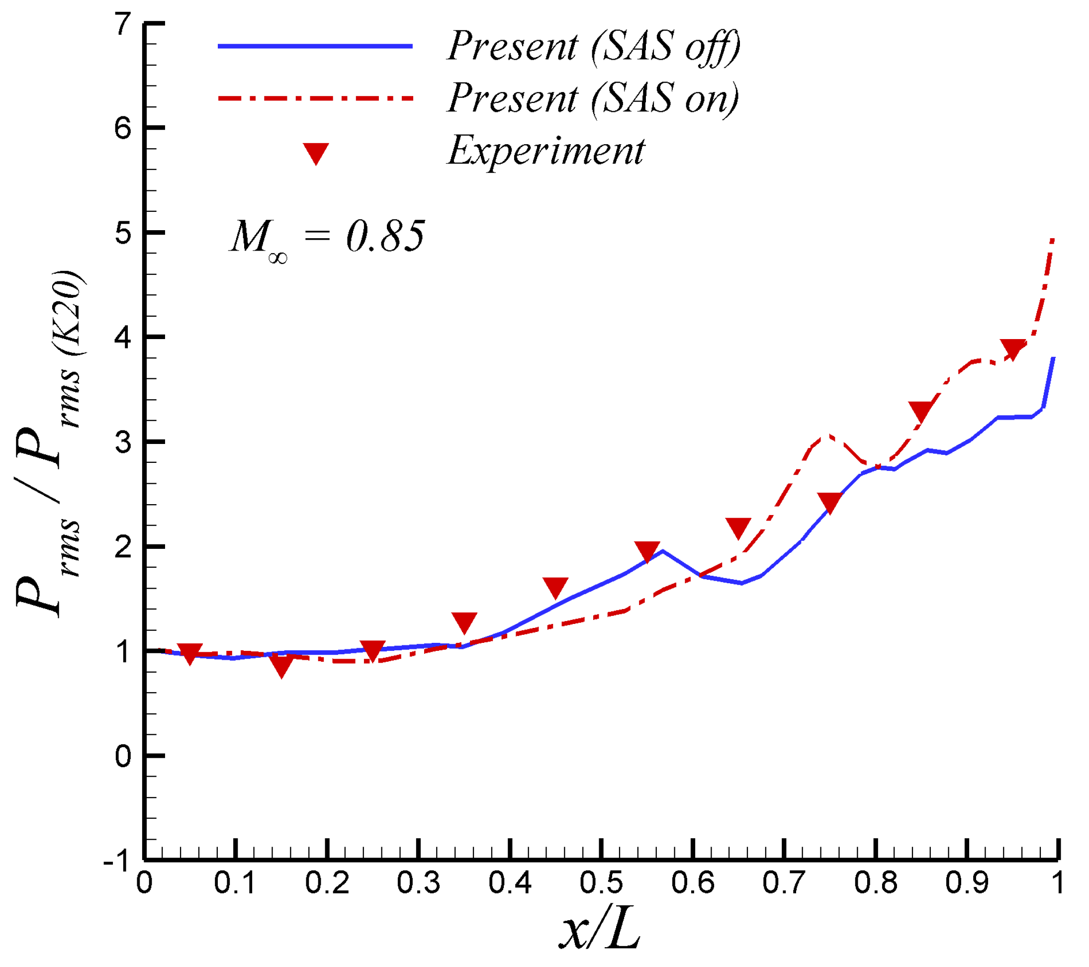
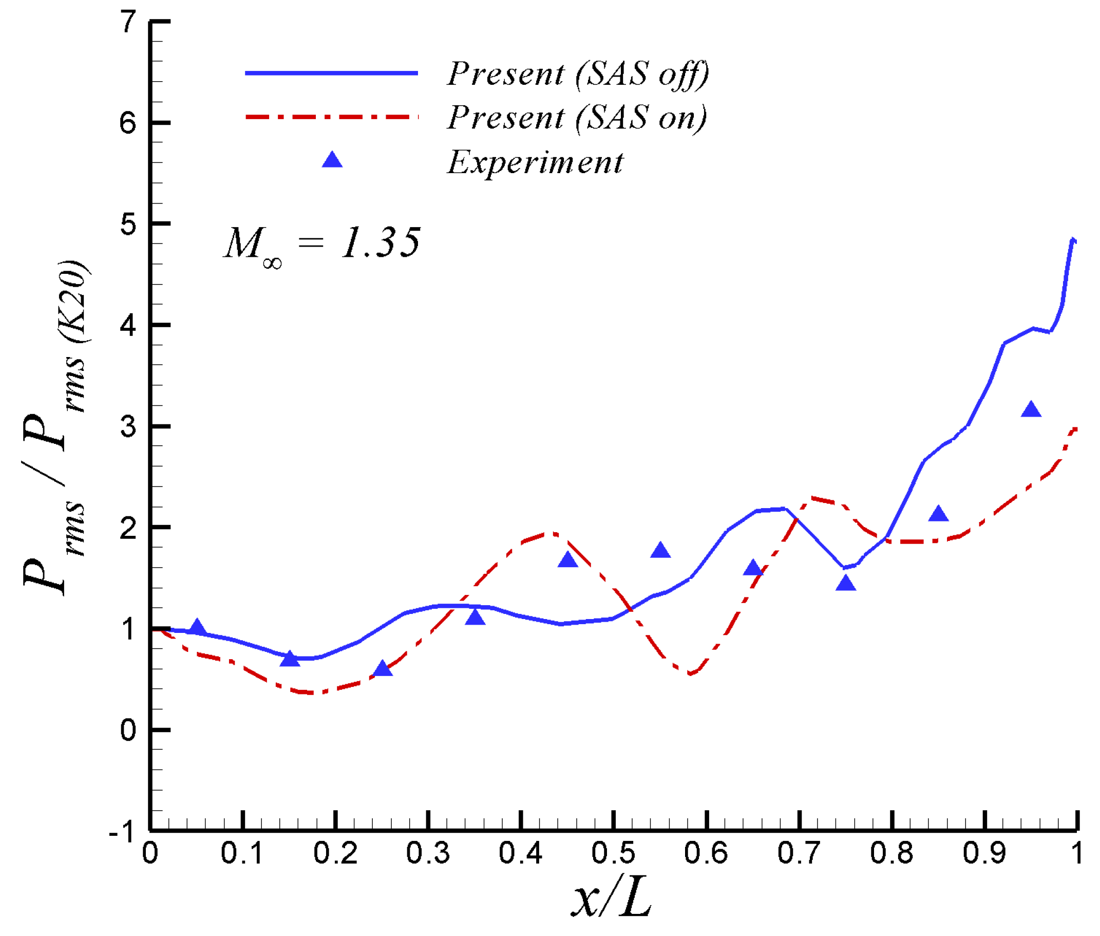
Results from the SAS model when switched on and off are shown in Figure 7 and Figure 8 at $M_{\infty }$ = 0.85 and 1.35, respectively. The agreement of the present URANS results exhibit a moderately better agreement with the experiments from [15] when the SAS model is active by the end of the cavity ceiling. It is hypothesized that the better performance of the SAS model at capturing experimental $P_{rms}$ in that rear cavity corner might be due to the presence of high turbulent kinetic energy, k, and consequently large values of the turbulence length scale, L, according to Equation (17) (as will be visualized later on). The extra term $Q_{SAS}$ (see Equation (16)) in the specific dissipation rate equation, $\omega$, is the sole adjustment to the SST model in Equation (11) to account for the von Karman length scale, $L_{\nu K}$, allowing the simulations to dynamically accommodate to resolve the large-scale motions (LSMs). Note that the term $Q_{SAS}$ is directly proportional to the square of the ratio L/$L_{\nu K}$. However, by taking into account zones away from the cavity rear corner, both options (off/on SAS) show similar performance.

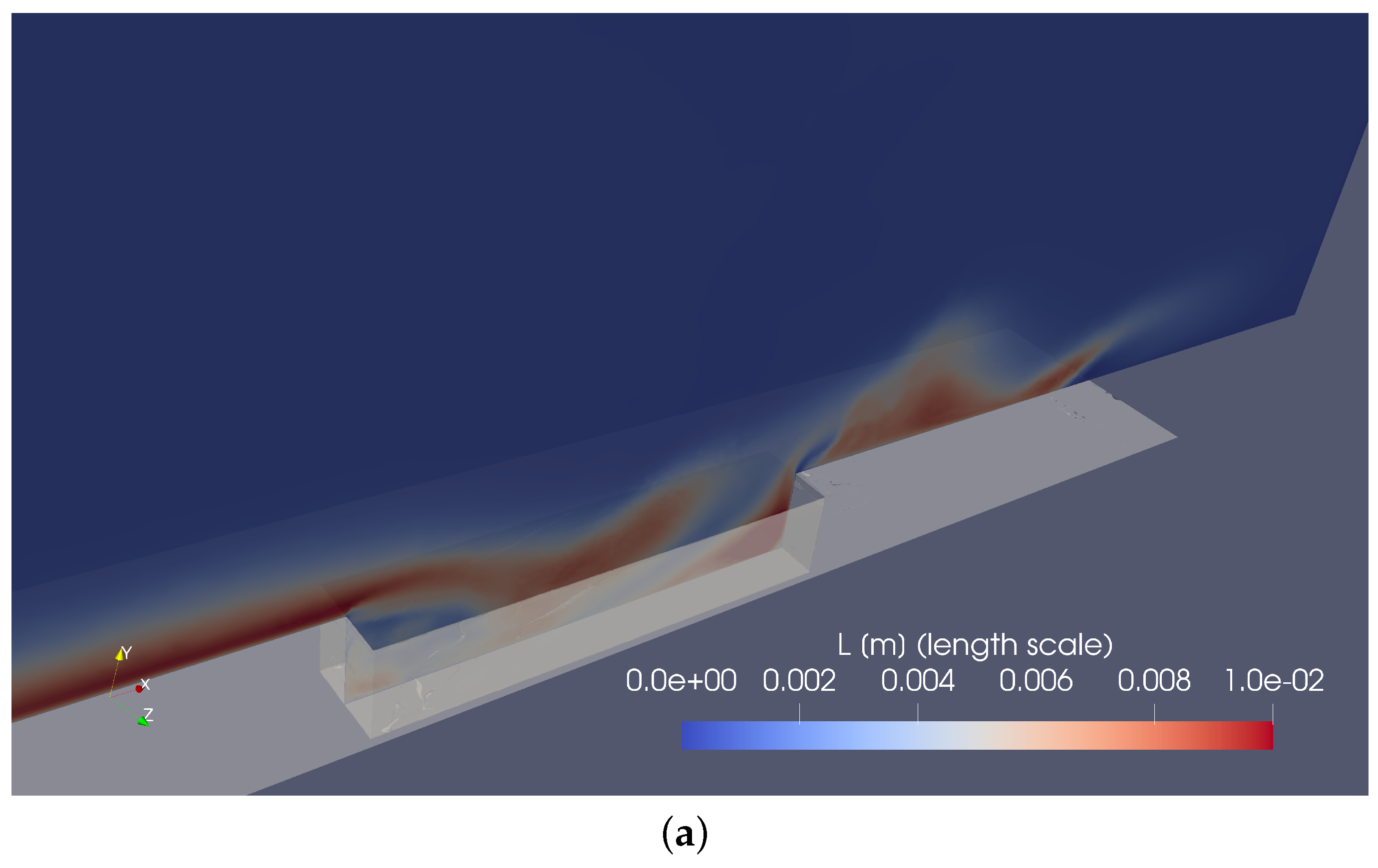
Furthermore, the corresponding iso-contours of instantaneous turbulence length scales, L, are shown in Figure 9a. The turbulence length scale is proportional to the square root of the turbulent kinetic energy, k, and inversely proportional to the specific dissipation rate, $\omega$. As seen in the centerline longitudinal plane of the cavity (Figure 9a), the maximum incoming length scale, L, is of the order of 0.01 m or $0.1D$, reaching values of $L\approx$ 0.012 m in the back bottom corner. These local large values of L at the rear corner cause (i) meaningful values for the $Q_{SAS}$, and (ii) changes in the spatial distribution of $\omega$ to better resolve LSMs, which could be the physical explanation of better capturing wall pressure fluctuations in Figure 7. Nevertheless, a deeper analysis should be carried out to shed light on this aspect, which is outside the present manuscript’s scope. The formation of the front vortex is also clearly seen, characterized by a flow recirculation zone (with low values of momentum and turbulent kinetic energy) bounded by large values of L (and turbulent kinetic energy, as well). A rear vortex system (highly energetic) is located at the end of the cavity at the bottom corner and characterized by significant turbulence length scale values. 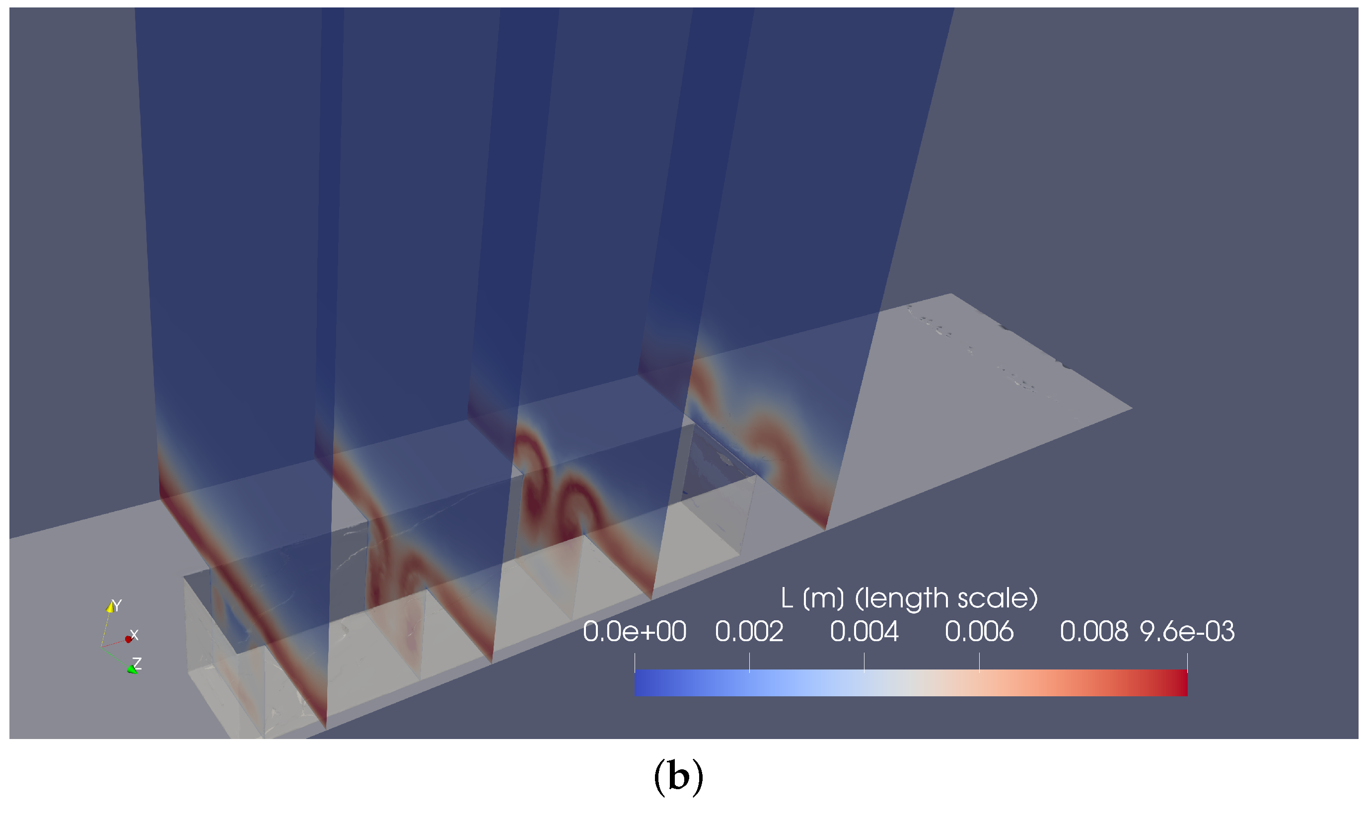Figure 9b exhibits four cross-sectional planes separated by a distance of approximately $1.5D$ with iso-contours of instantaneous turbulence length scales, L. The spatial sequence of the major horseshoe vortex formation can be observed.

In order to describe the different vortical structures observed in the cavity, we should mention the following categories, as described in [37], open-type cavity flow and closed-type cavity flow, which are determined according to the ratio $L/D$. At subsonic flow regimes, an open-type cavity ($L/D<7$) is represented by a shear layer that spans the entire cavity opening, and by a large recirculation zone inside the cavity itself [37]. On the other hand, closed-type cavities ($L/D>8$) are generally pictured by a shear layer generated at the front of the cavity that reattaches on the bottom of the cavity, without the presence of a large recirculation vortex in the center of the cavity. A transitional regime for rectangular cavities takes place in between. This seems to be the most appropriate category in which to class the present cavity at $L/D=5$. The reasons are supplied hereafter. Also, it is worth highlighting that the cavity is narrow because of $L/W=5$; thus, a completely three-dimensional geometry generates a different set of vortices. 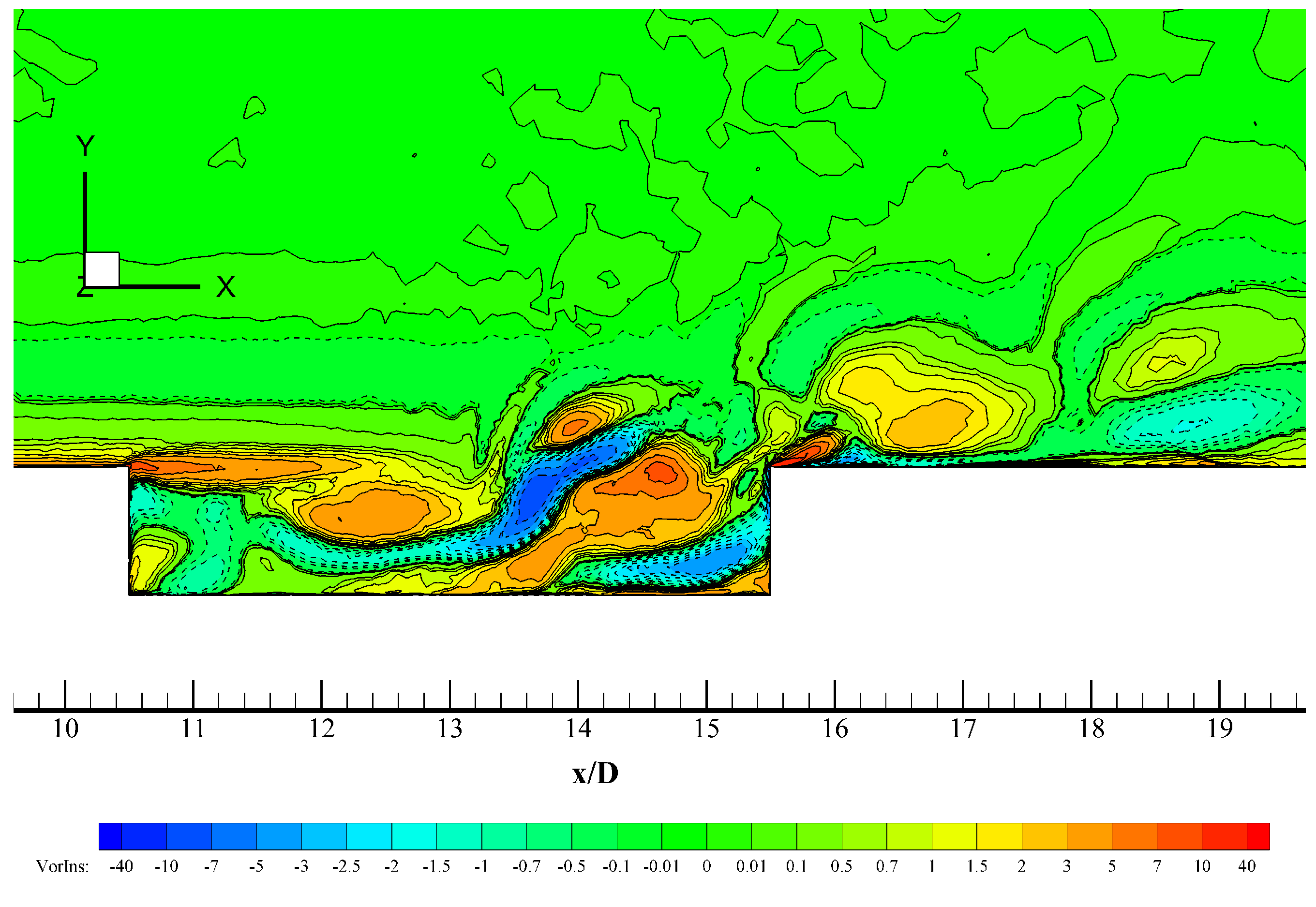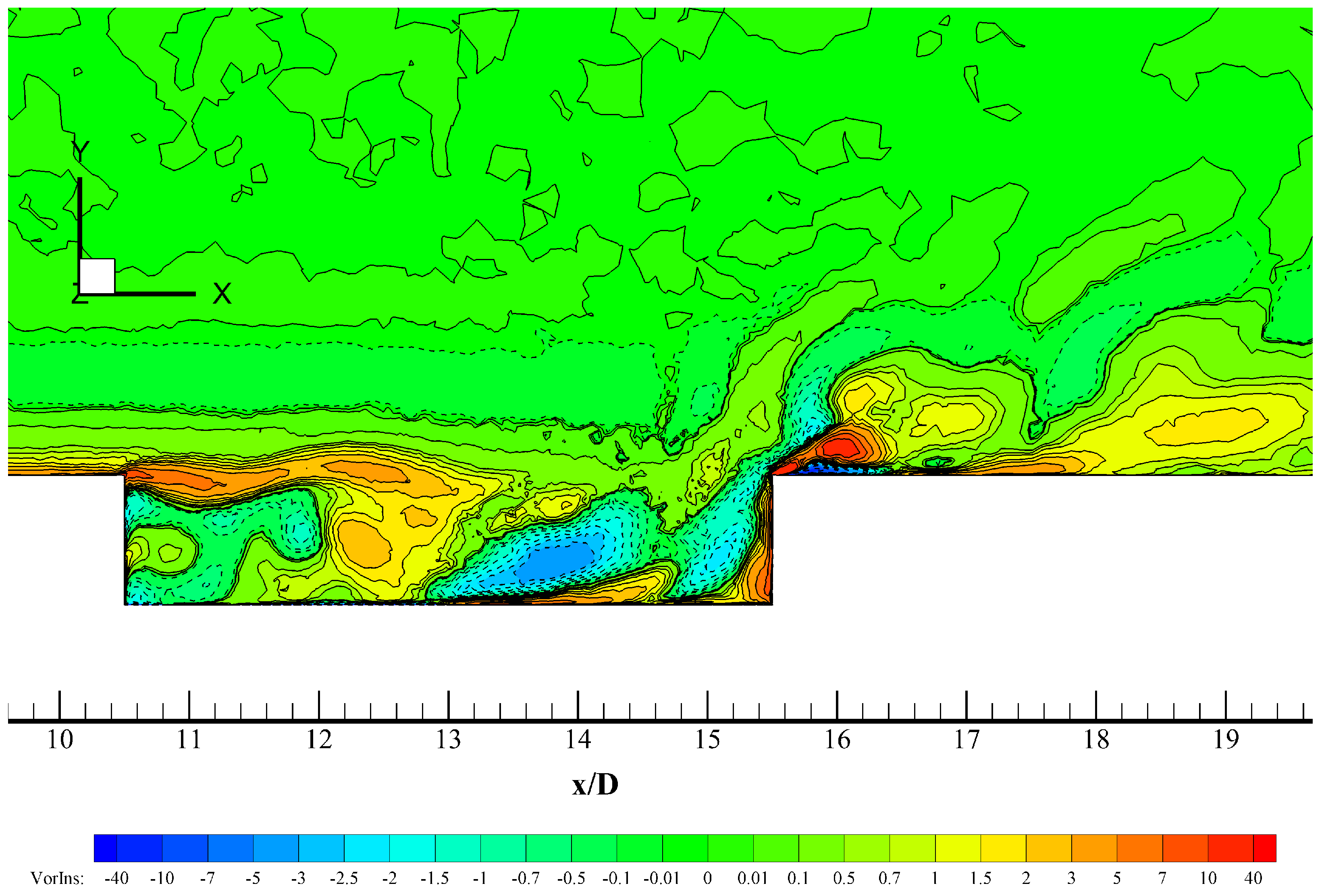Figure 10 shows contours of instantaneous spanwise vorticity. Positive isolines (inward vorticity vector or clockwise spin) are represented by solid curves; whereas, negatives isolines (outward vorticity vector or counter-clockwise spin) are represented by dashed curves. It can be seen in Figure 10 that the incoming turbulent boundary penetrates further into the cavity towards the ceiling. That incoming shear layer reattaches on the bottom of cavity, which is confirmed by Figure 11 (contours of instantaneous streamwise velocity normalized by the free-stream velocity). Two small recirculation zones with clockwise spins are observed in the front side (12 < $x/D$ < 13) and in the back side (14 < $x/D$ < 15) of the cavity in Figure 10. Particularly, the rear vortex transports fluid from the impinging shear layer on the cavity top downwards and towards the cavity bottom and viceversa, which is consistent with the findings of [37]. These phenomena induce two “curved” and elongated counter-clockwise vortices (or “banana-like” vortices) that contribute to the vertical mixing of turbulence inside the cavity. In particular, the vortex duplet located at the end of the cavity in the bottom corner is mainly responsible for turbulent kinetic energy generation, which in turns induces large local values of L, as previously explained. The $Q-criterion$ from [38] is implemented in this study to extract and visualize vortex cores via positive values, which describe regions of the flow where rotation dominates over strain. 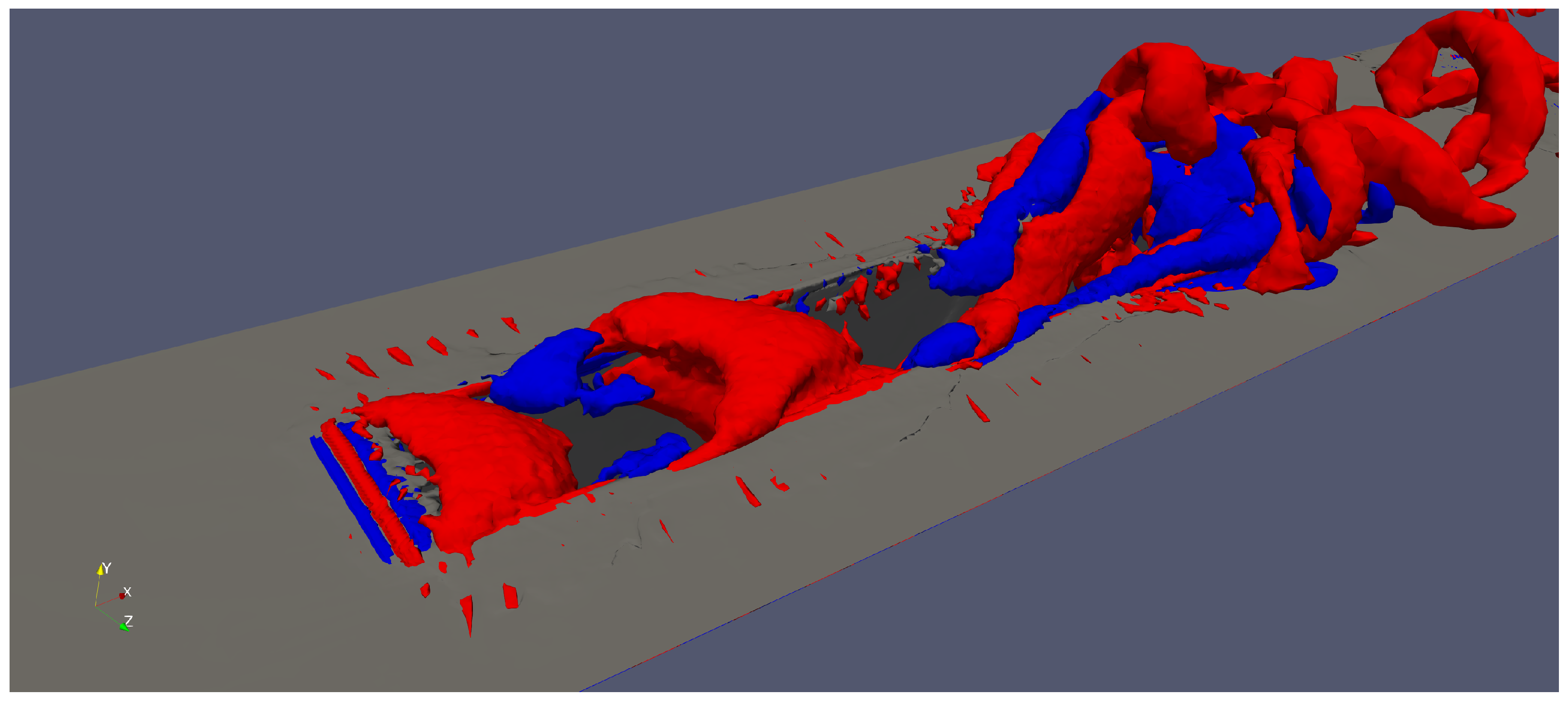On the other hand, negative iso-values of the $Q-criterion$ represent highly deformed flow regions. Iso-surfaces of the $Q-criterion$ (positive values in red and negative values in blue) are exhibited in Figure 12 at $M_{\infty }$ = 0.85. Focusing exclusively on the positive (red) iso-surfaces or vortex cores, the most energetic turbulent coherent structures emerge in three clearcut regions: (i) near the front region of the cavity, (ii) along the side cavity edges (see the presence of side vortices), and (iii) in the rear side of the cavity and downstream (vortex shedding). Highly energetic vortical coherent structures can also be observed in the cavity inside. These phenomena related to coherent structure dynamics are consistent with the findings and observations of [39]. The streamwise counter-rotating vortex pair described in Figure 9b is accurately captured by positive iso-surfaces of the $Q-criterion$. Interestingly, downstream of the cavity, where flow separates, the vortex adopts a horseshoe or hairpin shape (or omega-shaped vortices), as described by [40], with the typical leg, neck, and head. These coherent structures are commonly found in turbulent boundary layers, particularly in the log-region, which is mainly responsible for the generation of Reynolds shear stresses and turbulence production [40]. The vortex shedding downstream of the cavity resembles the jet in a cross-flow situation [41], where horseshoe vortices are continuously created by the interaction of the incoming shear layer with the vertical jet. It is hypothesized that the streamwise counter-rotating vortex pair at the end of the cavity lifts up low-speed fluid, interacting with the incoming shear layer over the cavity and mimicking the cross-flow jet problem. Highly strained flow (blue iso-surfaces) can be seen near vortex cores, predominantly in the cavity lateral sides and at the rear edge.

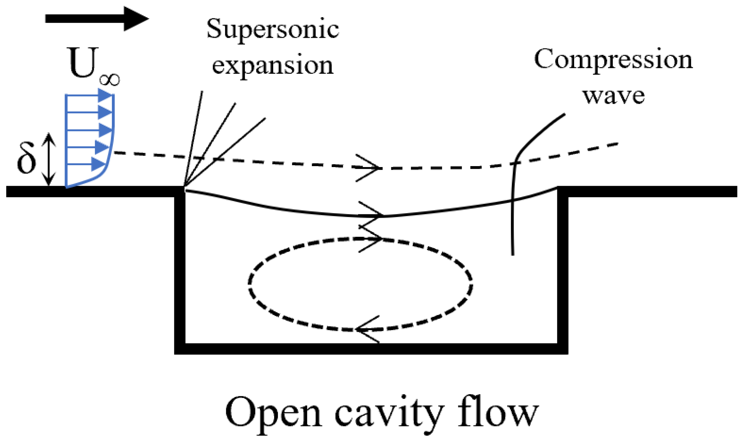
Turning to the Mach 1.35 case, it is important to emphasize the acoustic wave system generated when the incoming turbulent flow is supersonic. Figure 13 illustrates idealized time-averaged situations of the incoming supersonic boundary layer facing a rectangular cavity, adapted from [42]. According to Aradag and Knight [42], and similarly defined by [37] for incoming subsonic flow in rectangular cavities, one can define two major cavity types based on the $L/D$ ratio: open and closed cavity configurations. 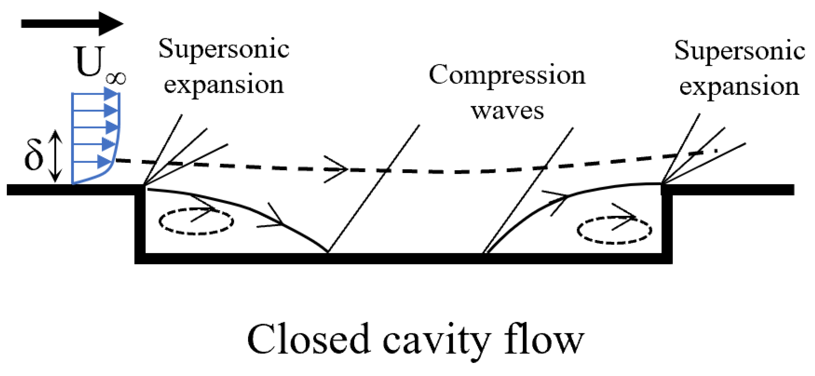In the open or “deep” cavity system (i.e., at low values of $L/D$), the turbulent free shear layer reattaches on the rear part of the cavity (see top image in Figure 13); therefore, creating a sole recirculation region in the mean flow. On the other hand, in the closed or “shallow” cavity (i.e., at large values of $L/D$), the shear layer reattaches on the cavity floor and the vortex system resembles a combination of a backward- and forward-facing step. While the flow physics in terms of open and closed cavities is somehow similar for incoming subsonic and supersonic flow; there is no general consensus about the critical $L/D$ values. For $L/D$ ratios greater than 13, it indicates closed cavity flow. While $L/D$ factors smaller than 10 indicate open cavity flow [42]. Furthermore, in Crook et al. [37] 8 and 7 are reported as these extreme $L/D$ values for incompressible flows. Clearly, one has to visualize the internal vortex system and the flow recirculation zone for better ascertaining whether one is dealing with open or closed cavity flows. Furthermore, the most important aspect to highlight in supersonic cavities is the presence of compression and expansion waves according to the cavity type [42], as depicted in Figure 13. 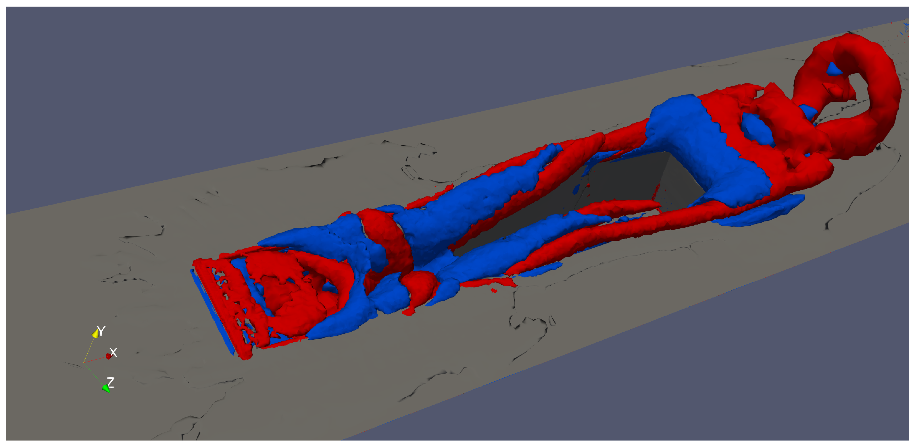Figure 14 depicts iso-surfaces of positive (vortex cores) and negative (highly deformed or strained flow) values of the $Q-criterion$ from [38] for the supersonic incoming flow, i.e., at $M_{\infty }$ = 1.35. The formation of horseshoe, hairpin-shaped, or omega-shaped vortices downstream of the cavity is evidently seen, as in the subsonic case in Figure 12. However, the distribution of volumes with either highly rotational (in red) or strained (in blue) flow is clearly different at $M_{\infty }$ = 0.85 and 1.35, respectively, which indicates that the vortex systems are rather distinctive in the supersonic case: most of the front side of the cavity is populated by vortex cores (rotational flow), whereas, by the rear cavity side and downstream, various zones coexist, either with a high level of rotation or deformation in a “twisted” fashion not observed in the subsonic case. The presence of highly strained flow downstream of the rear cavity could be linked to the significant unsteady expansion, which will be further discussed in this manuscript. 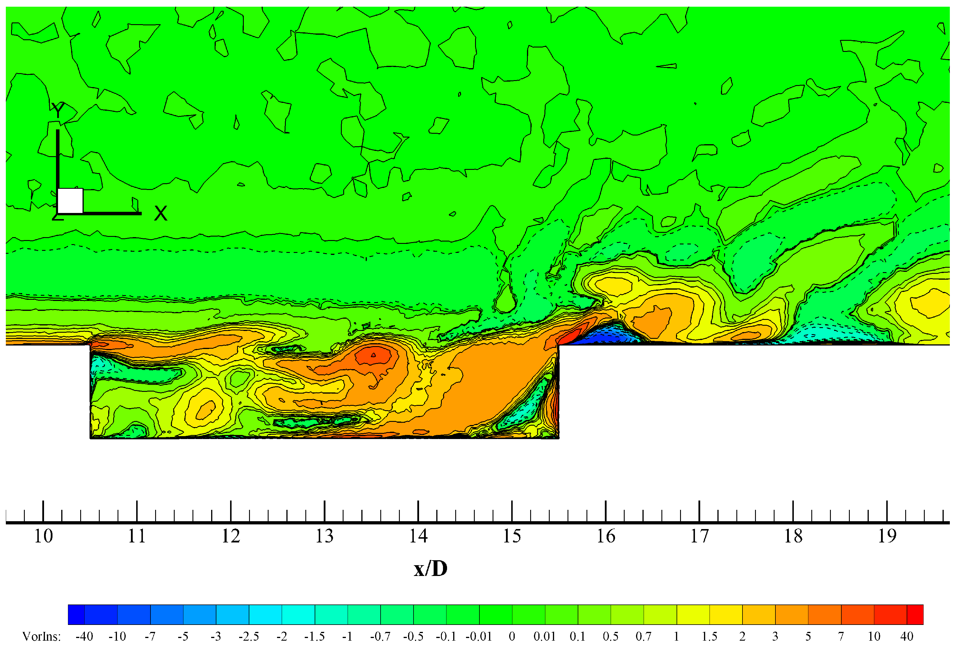In Figure 15, iso-contours of instantaneous spanwise vorticity are shown at $M_{\infty }$ = 1.35 and at the centerline plane $yx$ of the cavity (i.e., at $z/D$ = 0). As previously described, inward vorticity vectors or clockwise spin are represented by positive solid isolines, while outward vorticity vectors or counter-clockwise spin zones are represented by negative dashed curves. At this instant, two large vortical structures with opposite signs or a spanwise counter-rotating vortex pair (clockwise and counter-clockwise, respectively) are observed in the cavity center (12 < $x/D$ < 14.5). The incoming turbulent shear layer penetrates further, almost to the cavity bottom, and this clockwise spanwise vortex induces the nearby counter-clockwise vortex (by viscous effects and angular momentum conservation). At this point, the previously described instantaneous spanwise vortex pair leads to the generation of high levels of turbulent kinetic energy, wall-normal mixing, and strong pressure gradients (with minimum pressure at vortex centers) inside the cavity. Additionally, the instantaneous vortex pair promotes the vortex formation (with opposite sign) in the vicinity of the cavity via viscous effects. It is worth highlighting that for this narrow cavity ($L/W$ = 5) the turbulent flow generates highly unsteady three-dimensional vortical structures that significantly influence the cavity response. Figure 16 exhibits iso-contours of instantaneous spanwise vorticity at $M_{\infty }$ = 1.35 and at an off-centerline plane $yx$ (i.e., at $z/D$ = 0.25). The strong differences in instantaneous spanwise vorticity distribution at $z/D$ = 0.25 with respect to the cavity centerline plane ($z/D$ = 0) evidences the non-two-dimensional nature of this cavity configuration. 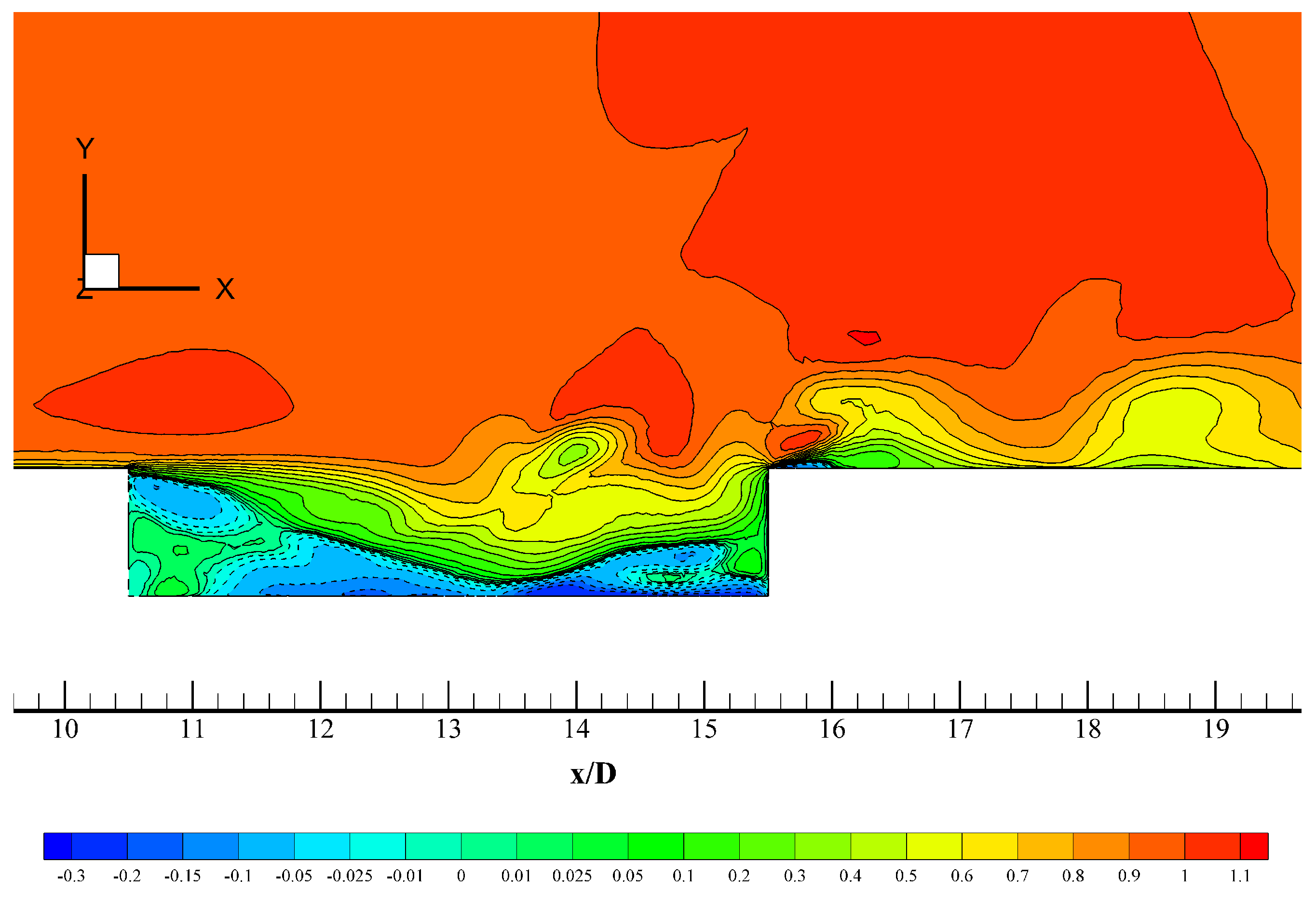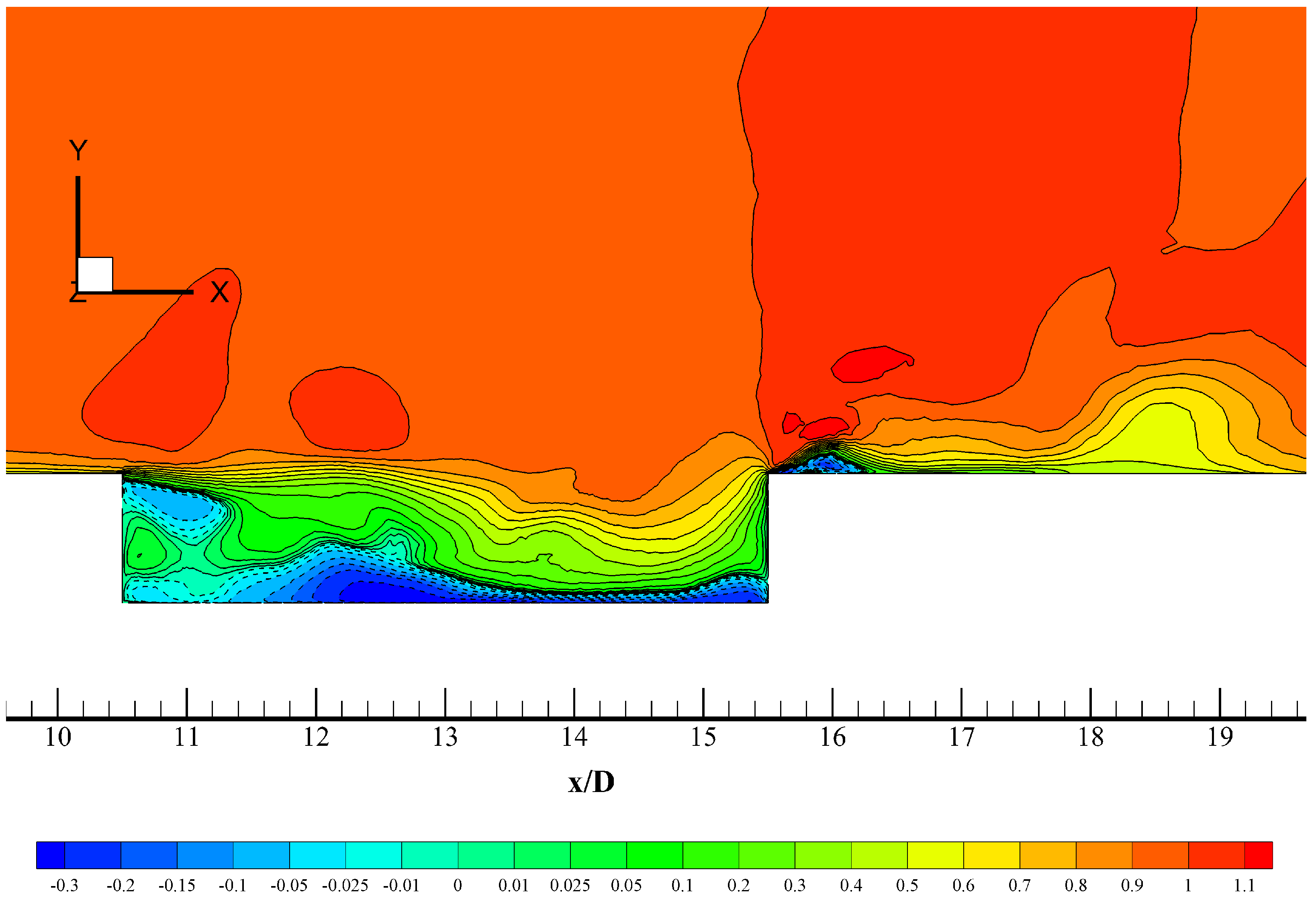In Figure 17, contours of instantaneous streamwise velocity normalized by the free-stream velocity are shown for the supersonic incoming flow case. The incoming turbulent shear layer develops from the front cavity edge, bends down into the first half (10.4 < $x/D$ < 13.4) due to pressure gradients, and impinges on the bottom. A clear backflow region is observed (blue) with negative values of the streamwise velocity. The red region just above the cavity edge indicates the presence of moderate instantaneous supersonic expansion or a favorable pressure gradient (FPG). In a similar manner, the flow strongly accelerates by the rear edge of the cavity. That strong supersonic expansion or FPG in the outer region and free-stream might be the reason for the presence of extremely strained flow at the trailing edge, represented by iso-surfaces of the $Q-criterion$ (in blue) in Figure 14. In addition, the very strong adverse pressure gradient (APG) generated by the rear cavity edge in the near-wall region is responsible for the downstream flow separation bubble. Outside of the rectangular cavity the flow is supersonic, whereas subsonic flow recirculating volumes take place inside [42]. Also, acoustic waves created due to the impingement of the turbulent shear layer at the rear wall of the cavity are able to propagate upstream through the subsonic region of the flow.

7. Conclusions

An evaluation of the Menter SST-SAS turbulence model in URANS of turbulent compressible flows and unstructured mesh is performed for a 3D acoustic cavity. The SAS approach is based on the use of the second derivative of the velocity that is highly active only on short scales. Therefore, this corresponds to an improvement over the original DES (detached-eddy simulation), which strongly depends on the grid spacing. Consequently, the SAS model exhibits simplicity, robustness, and moderate mesh dependency, which make it a good candidate for unstructured meshes in complex geometries. The scale-adaptive simulation model predicted fairly well the pressure fluctuation distribution over the subsonic cavity (M219), particularly at the rear part of the cavity where large values of L/$L_{\nu K}$ and $Q_{SAS}$ can be found in the near-wall region. Its performance was not as good for the supersonic case (free-stream Mach number of 1.35), which may be attributed to the presence of more complex high-speed flow (compression/expansion waves). The corresponding average discrepancies between the SAS numerical results and experiments by [15] were calculated to be approximately 0.13 $(P_{rms}/P_{rmsK20})$ and 0.26 $(P_{rms}/P_{rmsK20})$ units at Mach numbers of 0.85 and 1.35, respectively. However, a definite superiority could not be defined when the model was in “on” mode with respect to “off” mode, at least, based on the present acoustic cavity analysis. The selected problem configuration showed significant numerical challenges: highly 3D flow (deep cavity), sharp corners that induce strong adverse pressure gradients and boundary layer detachment, compressibility effects (presence of compression and expansion waves for the supersonic case), and an intricate vortex system. Furthermore, the SST-SAS model exhibits an adequate representation of the flow physics.

References

1. Mani, M.; Dorgan, A.J. A Perspective on the State of Aerospace Computational Fluid Dynamics Technology. Annu. Rev. Fluid Mech. 2023, 55, 431–457. [Google Scholar] [CrossRef]
2. Araya, G. Turbulence model assessment in compressible flows around complex geometries with unstructured grids. Fluids 2019, 4, 81. [Google Scholar] [CrossRef]
3. Paeres, D.; Lagares, C.; Araya, G. Assessment of Turbulence Models over a Curved Hill Flow with Passive Scalar Transport. Energies 2022, 15, 6013. [Google Scholar] [CrossRef]
4. Saltar, G.; Araya, G. Reynolds shear stress modeling in turbulent boundary layers subject to very strong favorable pressure gradient. Comput. Fluids 2020, 202, 104494. [Google Scholar] [CrossRef]
5. Menter, F.R.; Kolmogorov, D.K.; Garbaruk, A.V.; Stabnikov, A.S. Direct- and Large Eddy Simulations of Turbulent Flow in CS0 Diffuser on Resolved and Under-resolved Meshes. Flow Turbul. Combust. 2023, 110, 515–546. [Google Scholar] [CrossRef]
6. Menter, F.R.; Egorov, Y. A scale-adaptive simulation model using two-equation models. In Proceedings of the 43rd AIAA Aerospace Sciences Meeting and Exhibit, Reno, NV, USA, 10–13 January 2005. AIAA Paper AIAA2055-1095. [Google Scholar]
7. Menter, F.R.; Egorov, Y. The Scale-Adaptive Simulation Method for Unsteady Turbulent Flow Predictions. Part 1: Theory and Model Description. Flow Turbul. Combust 2010, 85, 113–138. [Google Scholar] [CrossRef]
8. Egorov, Y.; Menter, F.R.; Lechner, R.; Cokljat, D. The Scale-Adaptive Simulation Method for Unsteady Turbulent Flow Predictions. Part 2: Application to Complex Flows. Flow Turbul. Combust. 2010, 85, 139–165. [Google Scholar] [CrossRef]
9. Spalart, P.R.; Jou, W.-H.; Strelets, M.; Allmaras, S.R. Comments on the feas1ibility of LES for wings, and on a hybrid RANS/LES approach. In Proceedings of the First AFOSR International Conference on DNS/LES, Ruston, LA, USA, 4–8 August 1997. [Google Scholar]
10. Spalart, P.R.; Deck, S.; Shur, M.L.; Squires, K.D.; Strelets, M.; Travin, A.K. A new version of detached-eddy simulation, resistant to ambiguous grid densities. Theor. Comput. Fluid Dyn. 2006, 20, 181–195. [Google Scholar] [CrossRef]
11. Menter, F.R.; Kuntz, M. Adaptation of eddy-viscosity turbulence models to unsteady separated flow behind vehicles. In Symposium on the Aerodynamics of Heavy Vehicles: Trucks, Buses and Trains; McCallen, R., Browand, F., Ross, J., Eds.; Springer: Berlin/Heidelberg, Germany; New York, NY, USA, 2004. [Google Scholar]
12. Lawson, S.; Barakos, G. Review of numerical simulations for high-speed, turbulent cavity flows. Prog. Aerosp. Sci. 2011, 47, 186–216. [Google Scholar] [CrossRef]
13. Rowley, C.W.; Williams, D.R. Dynamics and control of high-Reynolds number flow over open cavities. Annu. Rev. Fluid Mech. 2006, 38, 251–276. [Google Scholar] [CrossRef]
14. Seker, A.E.; Zafer, B.; Gonzalez-Martino, I.; Yucetepe, M. Aeroacoustic investigation of transonic flow behavior in M219 deep cavity with passive flow control configurations. Phys. Fluids 2023, 35, 105117. [Google Scholar] [CrossRef]
15. Henshaw, M.J. M219 cavity case. In Verification and Validation Data for Computational Unsteady Aerodynamics; Tech. Rep. RTO-TR-26, AC/323/(AVT) TP/19; The Research and Technology Organization: Neuilly-sur-Seine, France, 2000; pp. 453–472. [Google Scholar]
16. Li, E.; Le, G.; Zhang, Y. Numerical simulation of supersonic cavity noise. AIP Conf. Proc. 2017, 1839, 020172. [Google Scholar]
17. Parra Rodríguez, J.A.; Abad Romero, M.A.; Huerta Chávez, O.M.; Rangel-López, L.R.; Jiménez-Escalona, J.C.; Diaz Salgado, J. Coherent Structures Analysis of Methanol and Hydrogen Flames Using the Scale-Adaptive Simulation Model. Energies 2023, 16, 7074. [Google Scholar] [CrossRef]
18. Kim, S.-J.; Choi, Y.-S.; Cho, Y.; Choi, J.-W.; Hyun, J.-J.; Joo, W.-G.; Kim, J.-H. Effect of Fins on the Internal Flow Characteristics in the Draft Tube of a Francis Turbine Model. Energies 2020, 13, 2806. [Google Scholar] [CrossRef]
19. Meana-Fernández, A.; Fernández Oro, J.M.; Argüelles Díaz, K.M.; Velarde-Suárez, S. Turbulence-Model Comparison for Aerodynamic-Performance Prediction of a Typical Vertical-Axis Wind-Turbine Airfoil. Energies 2019, 12, 488. [Google Scholar] [CrossRef]
20. Trivedi, C.; Cervantes, M.J.; Gandhi, B.K. Investigation of a High Head Francis Turbine at Runaway Operating Conditions. Energies 2016, 9, 149. [Google Scholar] [CrossRef]
21. Wiński, K.; Piechna, A. Comprehensive CFD Aerodynamic Simulation of a Sport Motorcycle. Energies 2022, 15, 5920. [Google Scholar] [CrossRef]
22. Hiller, S.; Seitz, P. Interaction between a Fluidic Actuator and Main Flow Using SAS Turbulence Modelling, AIAA 2006-3678. In Proceedings of the 3rd AIAA Flow Control Conference, San Francisco, CA, USA, 5–8 June 2006. [Google Scholar]
23. Rajkumar, K.; Tangermann, E.; Klein, M. Efficient Scale-Resolving Simulations of Open Cavity Flows for Straight and Sideslip Conditions. Fluids 2023, 8, 227. [Google Scholar] [CrossRef]
24. Morgan, K.; Peraire, J.; Peiro, J.; Hassan, O. The computation of 3-dimensional flows using unstructured grids. Comput. Methods Appl. Mech. Eng. 1991, 87, 335–352. [Google Scholar] [CrossRef]
25. Peiró, J.; Peraire, J.; Morgan, K. FELISA System Reference Manual. Part 1–Basic Theory; Swansea Report C/R/821/94; University of Wales: Swansea, Wales, 1994. [Google Scholar]
26. Peraire, J.; Morgan, K.; Peiró, J. Unstructured finite element mesh generation and adaptive procedures for CFD. In Proceedings of the Proceedings No: 464—Applications of Mesh Generation to Complex 3D Configurations, Loen, Norway, 24–25 May 1989; AGARD: Paris, France, 1990; pp. 18.1–18.12. [Google Scholar]
27. Hassan, O.; Morgan, K.; Probert, E.J.; Peraire, J. Unstructured tetrahedral mesh generation for three-dimensional viscous flows. Int. J. Numer. Methods Eng. 1996, 39, 549–567. [Google Scholar] [CrossRef]
28. Weatherill, N.P.; Hassan, O. Efficient three–dimensional Delaunay triangulation with automatic boundary point creation and imposed boundary constraints. Int. J. Numer. Methods Eng. 1994, 37, 2005–2039. [Google Scholar] [CrossRef]
29. Jameson, A.; Schmidt, W.; Turkel, E. Numerical simulation of the Euler equations by finite volume methods using Runge–Kutta timestepping schemes. AIAA Paper 1981, 81, 1259. [Google Scholar]
30. Harten, A.; Lax, P.D.; van Leer, B. On upstreaming differencing and Godunov-type schemes for hyperbolic conservation laws. SIAM Rev. 1983, 25, 35. [Google Scholar] [CrossRef]
31. Sørensen, K.A. A Multigrid Accelerated Procedure for the Solution of Compressible Fluid Flows on Unstructured Hybrid Meshes. Ph.D. Thesis, University of Wales, Swansea, UK, 2002. [Google Scholar]
32. Wilcox, D.C. Turbulence Modeling for CFD; DWC Industries, Inc.: La Canada, CA, USA, 2006. [Google Scholar]
33. Menter, F.R. Review of the shear-stress transport turbulence model experience from an industrial perspective. Int. J. Comput. Fluid Dyn. 2009, 23, 305–316. [Google Scholar] [CrossRef]
34. Spalart, P.R.; Rumsey, C.L. Effective Inflow Conditions for Turbulence Models in Aerodynamic Calculations. AIAA J. 2007, 45, 2544–2553. [Google Scholar] [CrossRef]
35. Araya, G.; Lagares, C. Implicit subgrid-scale modeling of a Mach-2.5 spatially-developing turbulent boundary layer. Entropy 2022, 24, 555. [Google Scholar] [CrossRef] [PubMed]
36. Lagares, C.; Araya, G. A GPU-Accelerated Particle Advection Methodology for 3D Lagrangian Coherent Structures in High-Speed Turbulent Boundary Layers. Energies 2023, 16, 4800. [Google Scholar] [CrossRef]
37. Crook, S.; Lau, T.; Kelso, R. Three-dimensional flow within shallow, narrow cavities. J. Fluid Mech. 2013, 735, 587–612. [Google Scholar] [CrossRef]
38. Hunt, J.C.R.; Wray, A.A.; Moin, P. Eddies, streams, and convergence zones in turbulent flows. In Studying Turbulence Using Numerical Simulation Databases, 2. Proceedings of the 1988 Summer Program; CTR: Stanford, CA, USA, 1988; pp. 193–208. [Google Scholar]
39. Mancini, S.; Kolb, A.; Gonzalez-Martino, I.; Casalino, D. Very-Large Eddy Simulations of the M219 Cavity at High-Subsonic and Supersonic Conditions. In Proceedings of the AIAA Scitech 2019 Forum, San Diego, CA, USA, 7–11 January 2019. AIAA 2019-1833. [Google Scholar]
40. Adrian, R.J.; Meinhart, C.D.; Tomkins, C.D. Vortex organization in the outer region of the turbulent boundary layer. J. Fluid Mech. 2000, 422, 1–54. [Google Scholar] [CrossRef]
41. Quiñones, C.; Araya, G. Jet in accelerating turbulent crossflow with passive scalar transport. Energies 2022, 15, 4296. [Google Scholar] [CrossRef]
42. Aradag, S.; Knight, D. Simulation of Supersonic Flow over a Cavity. In Proceedings of the 43rd AIAA Aerospace Sciences Meeting and Exhibit, Reno, NV, USA, 10–13 January 2005. AIAA 2005-848. [Google Scholar]
Figure 1. Experiment schematic and dimensions adapted from [15]: (a) right-side view, (b) top view, and (c) front view (flow from left to right in (a,b)).
Fluids 09 00092 g001
Figure 2. RMS of pressure fluctuations at the deep cavity ceiling and rig centerline (y = 0); from [15].
Fluids 09 00092 g002
Figure 3. Several schematics of the computational box and hybrid mesh: (a) lateral view with dimensions and boundary conditions (flow from left to right), (b) isometric view and half-plane of the cavity (flow from left to right), and (c) interior view (from upstream of the cavity).
Fluids 09 00092 g003aFluids 09 00092 g003b
Figure 4. Time variation of the total drag in the acoustic cavity at  M  = 0.85.
Fluids 09 00092 g004
Figure 5. Root mean square of pressure fluctuations in the acoustic cavity ceiling at  M  = 0.85 and 1.35: coarse and fine mesh results.
Fluids 09 00092 g005
Figure 6. Root mean square of pressure fluctuations in the acoustic cavity ceiling: comparison with experimental values at  M  = 0.85 and 1.35.
Fluids 09 00092 g006
Figure 7. Root mean square of pressure fluctuations in the acoustic cavity at  M  = 0.85.
Fluids 09 00092 g007
Figure 8. Root mean square of pressure fluctuations in the acoustic cavity at  M  = 1.35.
Fluids 09 00092 g008
Figure 9. Contours of the turbulence length scale over and inside the cavity: (a) longitudinal plane and (b) cross-sectional planes at  M  = 0.85.
Fluids 09 00092 g009aFluids 09 00092 g009b
Figure 10. Iso-contours of instantaneous spanwise vorticity in 1/s (flow from left to right) at  z / D =  0 and  M  = 0.85.
Fluids 09 00092 g010
Figure 11. Iso-contours of instantaneous streamwise velocity normalized by the free-stream velocity (flow from left to right) at  z / D =  0 and  M  = 0.85.
Fluids 09 00092 g011
Figure 12. Iso-surfaces of  Q c r i t e r i o n , positive values in red (vortex cores), negative values in blue (highly deformed flow regions), at  M  = 0.85.
Fluids 09 00092 g012
Figure 13. Types of supersonic cavity flows.
Fluids 09 00092 g013aFluids 09 00092 g013b
Figure 14. Iso-surfaces of  Q c r i t e r i o n , positive values in red (vortex cores), negative values in blue (highly deformed flow regions), at  M  = 1.35.
Fluids 09 00092 g014
Figure 15. Iso-contours of instantaneous spanwise vorticity in 1/s (flow from left to right) at  z / D =  0 and  M  = 1.35.
Fluids 09 00092 g015
Figure 16. Iso-contours of instantaneous spanwise vorticity in 1/s (flow from left to right) at  z / D =  0.25 and  M  = 1.35.
Fluids 09 00092 g016
Figure 17. Iso-contours of instantaneous streamwise velocity normalized by the free-stream velocity (flow from left to right) at  z / D =  0 and  M  = 1.35.
Fluids 09 00092 g017
Disclaimer/Publisher’s Note: The statements, opinions and data contained in all publications are solely those of the individual author(s) and contributor(s) and not of MDPI and/or the editor(s). MDPI and/or the editor(s) disclaim responsibility for any injury to people or property resulting from any ideas, methods, instructions or products referred to in the content.