Abstract
The rapid growth of drone use in urban areas has prompted authorities to review airspace regulations, forcing drone manufacturers to anticipate and reduce the noise emissions during the design stage. Additionally, micro air vehicles (MAVs) are designed to be aerodynamically efficient, allowing them to fly farther, longer and safer. In this study, a steady aerodynamic code and an acoustic propagator based on the non-linear vortex lattice method (NVLM) and Farassat’s formulation-1A of the Ffowcs Williams and Hawkings (FW-H) acoustic analogy, respectively, are coupled with pymoo, a python-based optimization framework. This tool is used to perform a multi-objective (noise and aerodynamic efficiency) optimization of a 20 cm diameter two-bladed rotor under hovering conditions. From the set of optimized results, (i.e., the Pareto front), three different rotors are 3D-printed using a stereolithography (SLA) technique and tested in an anechoic room. Here, an array of far-field microphones captures the acoustic radiation and directivity of the rotor, while a balance measures the aerodynamic performance. Both the aerodynamic and aeroacoustic performance of the three different rotors, in line with what has been predicted by the numerical codes, are compared and guidelines for the design of aerodynamically and aeroacoustically efficient MAV rotors are extracted.
1. Introduction
The straightforward and simple design of quadcopter micro air vehicles (MAVs) has contributed greatly to their growing popularity in recent years [1]. The versatility and utility of drones in diverse sectors is highlighted by their use in a variety of applications, such as delivery of goods [2], photogrammetric surveying [3], and facility surveillance [4,5,6]. The deployment of micro air vehicles in densely populated urban environments has necessitated regulatory oversight, resulting in the enactment of usage restrictions [7]. It is expected that future regulations will also introduce increasingly stringent noise limits, a development which is already forcing manufacturers to incorporate noise reduction strategies at the early stages in the design process. As a result, there is a growing demand for methodologies that can quickly and accurately predict the aerodynamic and aeroacoustic performance of micro air vehicles, which is critical for optimizing their characteristics within an acceptable timeframe. However, the complexity of the airflow interactions experienced by these drones presents a significant challenge. Accurately modeling all the aeroacoustic noise sources with methods that are both rapid and reliable remains a complex task, reflecting the intricate nature of the airflow dynamics associated with MAVs. The close proximity of the fast rotating rotors to each other [8] and to the body [9,10,11] generates highly coupled aerodynamic and aeroacoustic interactions that scatter an unpleasant noise to human ears. Shaffer et al. [12] suggested that quadcopter drone noise is more annoying than road traffic and aircraft noise because of its particular tonal and high-frequencies broadband noise components. While the former consists of a tonal peak at the blade-passing frequency (BPF) and its harmonics and is mainly associated with stationary loading, the latter is related to turbulence interacting with the airfoil [13]. They can all be predicted quite accurately by high-fidelity approaches such as DNS (direct numerical simulations) or LES (large eddy simulations), which are however computationally expensive and far too slow for industrial purposes. For such targets, low-fidelity aerodynamic codes such as BEMT (blade element momentum theory) or VLM (vortex lattice method)/VPM (vortex particle method) combined with aeroacoustic models are preferred. The tonal noise of rotating systems has been studied extensively since the appearance of aircraft propellers and helicopters rotors. Gutin [14] holds the distinction of being the first researcher to successfully compute the first harmonics of the steady loading noise for a stationary propeller. This significant contribution is the reason why steady loading noise is often referred to as Gutin noise. In parallel, Ernsthausen and Deming first acknowledged the significance of the thickness noise. Ernsthausen [15] explained its origin and characteristics, Deming [16] formulated the problem theoretically. Building upon these studies, Farassat and Succi [17] delved deeper into these two phenomena. They developed formulations 1 and 1A of the Ffowcs Williams and Hawkings (FW-H) acoustic analogy [18], which have become instrumental in the field. Notably, the formulation-1A has been used extensively to predict the tonal noise emitted by rotary wings, such as helicopter rotors and aircraft propellers. During the last decade, this methodology has also demonstrated its effectiveness in predicting the tonal noise from MAV rotors, as evidenced by multiple studies [19,20].
The first model for broadband noise was developed by Ffowcs Williams and Hall [21], who calculated the trailing edge noise component from turbulent eddies convected at the trailing edge using the Green’s function of a semi-infinite plate. Amiet [22,23] decomposed the various sources to obtain the scattered surface pressure distribution. Roger and Moreau [24,25,26] extended Amiet’s work by incorporating the effects of leading-edge back-scattering. In parallel, the BPM (Brooks, Pope, and Marcolini) model [27], developed by Brooks, Pope, and Marcolini from Ffowcs Williams and Hall’s solution and empirical data from NACA0012 airfoil tests, was initially developed for airfoil noise and later adapted for propellers using strip theory [13].
These models have accurately predicted broadband noise for helicopter rotors [28,29], automotive fans [30,31,32,33] and wind turbines [34,35,36,37], which involve moderate-to-high Reynolds numbers and fully turbulent boundary layers. However, for micro air vehicles operating at lower Reynolds numbers, the boundary layer dynamics differ, being not fully turbulent, prone to laminar separation, and the formation of laminar separation bubbles [38,39,40], leading to more challenging broadband noise predictions and reducing the accuracy of these methods for smaller rotors.
In the present study, the attention is primarily focused on the blade passing frequency (BPF) noise, as it has been observed that the tonal noise peaks are typically more prominent than the broadband noise in the context of two-bladed 20 cm diameter rotors [41]. This approach prioritizes the analysis of BPF noise as the initial step in understanding the acoustic characteristics of such rotors.
The susceptibility of the boundary layer to separate and the importance of viscous friction at the characteristic Reynolds numbers of MAVs (∼–105) results in a reduction in the aerodynamic efficiency of the propellers [42]. Consequently, the airfoil lift coefficient slopes may be far off the slope predicted by the thin airfoil theory. Winslow et al. [43] explained through computational studies the origin of the two different slopes in the “linear region” appearing on the NACA0012 airfoil at : from 0° to 8°, a separation bubble travels from the trailing edge to the leading edge, modifying the laminar-to-turbulent transition. After 8°, a trailing edge separation bubble is formed until full stall at around 12°–14°. These phenomena also cause lower airfoil (and rotor) efficiencies and make rotor aerodynamic predictions more challenging. Due to the aforementioned reasons, and because MAVs rely on lightweight batteries with relatively low energy storage, rotor aeroacoustics optimizations must be tightly coupled with the aerodynamic optimizations to create stealthier and high endurance rotors.
In the past and starting from a two-blade standard propeller, Vogeley [44] experimentally reduced the aircraft propeller noise by changing the number and planform of the blades. Together with the position of the engine exhaust system, these modifications induced a decrease in the operating rotational speed and an abatement of the emitted sound, without compromising its aerodynamic performance.
With the advent of optimization algorithms and the increase in computational power, multi-objective optimizations started to be performed on fans [45,46,47] and on general aviation aircraft propellers [48,49,50,51,52,53,54,55,56].
Pagano et al. [50,57] used a design of experiment (DOE) technique to optimize the aerodynamic efficiency in cruise condition (at Mach number = 0.58), calculated by means of CFD simulations, and the noise emitted at take-off, when the thrust is maximum and the aircraft is closer to the ground. Although the code was able to predict both tonal and broadband noise components using the Farassat formulation-1A of the Ffowcs Williams–Hawkings acoustic analogy and trailing edge noise semi-empirical models, respectively, the optimization results demonstrated that the noise reduction was mainly led by the reduction in the tonal noise.
Optimizations have also been performed on helicopter rotors [58,59,60,61,62,63]. Bu et al. [61] coupled a RANS solver, a penetrable data surface (PDS) formulation of the FW-H acoustic analogy, with a hierarchical kriging (HK) optimization procedure to optimize the noise emitted without decreasing the efficiency in hover. The airfoil shape and also the blade chord, pitch, and sweep distributions were modified.
Due to the recent developments of MAVs, MAV rotor optimizations have been carried out [64,65,66,67,68,69,70,71]. Serré et al. [67] used BEMT simulations coupled with the Farassat formulation-1A and semi-empirical broadband noise models to predict hover efficiency, tonal noise, and broadband noise, respectively. The optimizations involved changes in airfoil, chord and pitch distributions. However, the resulting geometries differed from the more traditional optimized rotor geometries. In order to optimize the hover efficiency, Gessow [72] demonstrated through the momentum theory/BEMT that the ideal rotor should have a pitch distribution that follows a hyperbolic equation, resulting in a linear distribution of lift. Additionally, to ensure that each blade section operates at the optimum lift-to-drag ratio, the local blade solidity and chord should also follow a hyperbolic equation. The chord therefore tends to infinity at the root of the blade, making it impossible to replicate in reality. Nevertheless, a linear approximation of both chord and pitch distributions in the region near the blade tip showed aerodynamic performance comparable to that of the rotors with hyperbolic chord and pitch distributions.
Since BEMT simulations (used in [67,68,69]) do not predict the aerodynamic blade vortex interaction and the blade–wake interaction, the need for more accurate optimizations has pushed the authors to perform multi-objective optimizations using middle fidelity, but with a relatively fast, steady non-linear vortex lattice method (S-NVLM) code [20,73] coupled to a Farassat formulation-1A code. Furthermore, the optimization process includes manufacturing and operational constraints which render present results more useful in practice. Finally, optimizations are verified a posteriori using experiments, which is rarely reported in the literature and helps to gain further insight into the advantages and disadvantages of the optimization procedure.
The aim of this paper is thus to first describe a multi-objective optimization of MAV rotors subject to manufacturing and operational constraints using middle fidelity numerical tools. The optimized geometries are then analyzed both numerically and experimentally. The numerical procedure permitting to capture the aerodynamic performance of the rotor and its tonal noise is presented in Section 2, followed by the optimization setup used to obtain the final three optimized MAV rotors in Section 2.5. The results are then presented: first the optimization results in Section 3.1, then the optimized rotors and the unsteady simulations in Section 3.2, followed by the experimental results in Section 3.3 and a conclusion in Section 4.
2. Numerical Methods
As outlined in the Section 1, drone manufacturers are being pushed by stricter regulations to design MAV rotors that not only comply with current and future noise regulations, but that can also fly longer and farther to accomplish different missions. The development of numerical tools and procedures to predict and optimize the aerodynamic and aeroacoustic performance of rotors is essential to avoid the classical (and expensive) experimental trial-and-error approach. The optimization procedure, used in this work and described in Section 2.4, relies on an aerodynamic solver (Section 2.1) and an aeroacoustic propagator (Section 2.2).
2.1. Aerodynamic Solver: Non-Linear Vortex Lattice Method
The NVLM code developed by Jo et al. [19,73] is used here to calculate the performance and the airflow properties induced by MAV rotors in hovering and isolated conditions (Figure 1). Two different solvers of the same NVLM code are used: a steady one, which models the wake as an uncontracted helicoid, and an unsteady one, which models the wake by means of free vortex particles (Figure 1). The former is used during the optimization phase because of its computational speed, while the latter is used for ad hoc verification of the performance of the optimal geometries.
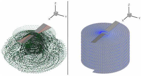
Figure 1.
On the left, an unsteady simulation snapshot with blade lattices, wake lattices (the red panels), and vortex particles (the green dots). On the right, a steady simulation snapshot of the blade lattices and the prescribed wake lattices (the blue panels).
Both solvers are based on the potential flow theory which assumes that the flow is incompressible , inviscid , and irrotational . The last hypothesis leads to a conservative vector field, that is, the velocity vector is equal to the gradient of a velocity potential, noted as :
Equation (1) satisfies Laplace’s equation . Since Laplace’s operator is linear, multiple velocity potentials can be linearly added to create more complex flows.
In the case of the VLM, the final flow-field is a combination of elementary vortex rings (or lattices) with constant strength . Since the rotor blade is considered to be thin (with respect to the chord), the 3D blade camber line is discretized into lattices (where and are the number of lattices along the chord and span, respectively) and the circulations of the vortex rings are noted as [74] (see Figure 2). These vortices generate an induced velocity at all points in space and must satisfy the non-penetrating condition at the blade surface. As shown in Figure 2, each vortex lattice follows the – rule [74]: the leading vortex ring segment is placed at of the geometric cell chordwise length, and a collocation point is placed at of the chordwise cell length. In this point, noted , the non-penetrating condition is applied. The velocity induced by a vortex ring at the collocation point is computed by considering the contribution of all the four vortex edges thanks to the Biot–Savart law [74].
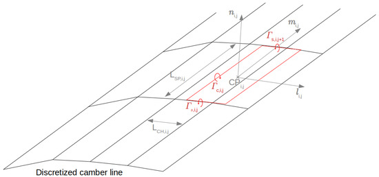
Figure 2.
A typical VLM blade discretization, with the vortex ring (in red).
The total number of lattices N is equal to the number of rotors multiplied by the number of rotor blades and the number of lattices per blade . As the circulations are the unknowns of the problem, the influence coefficients are initially computed by considering the velocity induced by the four vortex segments of lattice q onto the collocation point of lattice p, with . For each lattice p, the non-penetrating flow condition can be written as follows:
By moving the terms to the right-hand side, the following system is obtained:
is the velocity induced by all wake vortices at the collocation point of lattice of index p, the velocity induced at lattice p by the rotation of the blade, is the freestream velocity vector, and the vector normal to the lattice.
A sectional non linear correction on is then performed using the XFOIL [75] lookup tables to account for the low Reynolds number induced non-linearities (for more information, please refer to Li Volsi [76]).
As the wake affects the velocity induced on the blade, and therefore the rotor performance through the term , several methods have been developed to propagate the wake behind the trailing edge of the blades. As previously mentioned, two different wake models are used in this work: a steady one, which models the wake as a prescribed and uncontracted helicoidal wake, and an unsteady one, more accurate and computationally more expensive, that uses a vortex particle method (VPM).
On the latter, Lagrangian-described vortex particles (or blobs) are shed at each timestep from the trailing edge of the blades. Their total number depends on the number of blade spanwise lattices, the angle-defined timestep (referred to as step angle afterwards), and the number of total revolutions. They are characterized by a constant circulation and allow us to reconstruct the vorticity field at a given location x anywhere near the rotor through the following formula:
with:
- the location of the ith particle;
- t the physical time;
- is the regularized vorticity distribution function within the core of the particle ( is the core size).
Since the vortex particles constantly influence each others and their number increases throughout the simulation, the computational cost is proportional to , but the implementation of a Fast Multipole Method has reduced it to [19].
The steady solver, on the other hand, is based on a prescribed wake model [77]. The discretization of the helical wake is fixed from the beginning of the simulation and depends on the blade spanwise lattices, the step angle (that, in this case, defines the angular spacing between two consecutive rows of wake lattices), and the number of revolutions to simulate. The induced velocity is calculated at each spanwise section j by using Biot–Savart’s law and the blades’ lattices circulations. In the present prescribed wake model, the helix pitch is supposed to be constant from the inboard to the outboard part of the helix, the rotor induced velocity is calculated by averaging all the spanwise induced velocities and used to set the helix pitch. To satisfy the 3D Kutta condition at the trailing edge of the blades, the circulation of the first row (noted k) of wake lattices must be equal to the circulations of the trailing edge lattices:
The other wake lattice rows take the same circulation strength as the first row:
is the total number of wake lattice rows.
In the next iteration, the new averaged spanwise-induced velocity projected on the rotational axis is calculated by taking into account the new blade and wake lattice circulations, so that the new helix pitch is calculated. As this is a steady simulation and the helix discretization is fixed at the beginning of the computation, the calculation stops when the thrust coefficient is converged.
The main outputs of both solvers are the rotor thrust and torque and the blade loading distribution (this is one of the inputs of the acoustic propagator presented in Section 2.2). The aerodynamic efficiency is calculated through the figure of merit [78] (FM, Equation (7)), which depends on the thrust T, torque Q, rotational speed , air density , and rotor radius R:
The simulation parameters, shown in Table 1 and chosen for the optimizations, are sufficient to capture with a good accuracy both aerodynamic and aeroacoustic performance of the rotors, while limiting the computational time (please refer to Jo et al. [19] and Li Volsi [76] for the validation of the code). As previously explained, the step angle defines the geometric discretization of the helical wake in the steady simulations, whereas in the unsteady simulations, it defines the time discretization. Both FM and BPF SPL are calculated by taking into account the last five revolutions in the unsteady simulations.

Table 1.
Simulation parameters.
2.2. Aeroacoustics Solver: Farassat Formulation-1A
To capture the tonal noise emitted by MAV rotors, Farassat’s formulation-1A of the Ffowcs Williams and Hawkings acoustic analogy has been implemented in the NVLM code on both unsteady and steady solvers [20,79]. The considered acoustic sources are as follows:
The thickness noise depends on the rotor geometry presented in Figure 3 (through the normal vector and the integral on the blades surface ), the rotational speed (velocity and Mach vector ), the position of the observer ( is the position of the observer and is the observer vector that defines the position of the observer from a radiating point in the geometry), and the properties of the air (density and speed of sound c):
with:

Figure 3.
A typical pressure distribution (depicted by the red arrows) along the mean camber line of the rotor blades (on the left) used to compute the loading noise and the 3D-modeling of the rotor blades (on the right) used to compute the thickness noise.
The loading noise depends on the loading distribution l and its derivative on the blade surface (in the case of the present NVLM code, on the mean camber line of the blade, see Figure 3). These variables, calculated beforehand by the aerodynamic code, are the input of the following equation:
with
This formulation is applied to solid boundaries (the blades) for the noise calculation. Therefore, only thickness and loading noise are radiated here, while the quadrupole term due to the wake turbulence is neglected.
The NVLM code used in this work calculates the pressure jump between the suction and pressure sides on the blade mean camber line due to the thin airfoil approximation. This pressure difference distribution is then used to compute the loading noise (see Figure 3).
Since lattices do not radiate to the observer at the same time, the retarded time () must be calculated for each lattice, and the acoustic pressure evaluated at this retarded instant. The contribution of each lattice is then taken into account to calculate the whole rotor acoustic pressure. It is worth noting that for both loading and thickness noises, the near-field terms (characterized by an amplitude decay of ) and far-field terms ( decay) are separated.
Once the temporal signal is calculated, the fast-Fourier-transform (FFT) is computed and the BPF SPL captured. Note that the frequency sampling depends on the previously introduced step-angle (Section 2.1). The BPF SPL is the input required by the optimization algorithm.
2.3. Optimization Algorithm and Framework
Optimization techniques play a pivotal role in diverse applications, ranging from engineering to machine learning, finance, and many more [80]. These techniques focus on finding the best solution(s) within a defined parameter space and by satisfying the constraints set for a given problem (Equation (11)).
where is the vector constituted by the design variables that are allowed to change during the optimization. Traditional gradient-based optimization techniques have proven their effectiveness in searching the optimized parameters in single-objective optimizations.
However, this minimum may be local, rather than global. Gradient-based algorithms are, in fact, very sensitive to the initial guess. If it is located next to a local minimum, this family of algorithms will generally become stuck at the local minimum.
Real-world problems often require multi-objective optimizations, which do not converge to a singular, global optimal solution but rather yield a set of Pareto optimal solutions. This complexity is compounded when the gradient of the objective function is challenging to compute or unavailable. To address this, gradient-free algorithms have been developed, offering a viable approach to calculate Pareto optimal solutions in the absence of gradient information.
In this work, genetic algorithms (GA) are employed to simultaneously optimize two distinct and competing objectives. These algorithms, inspired by Charles Darwin’s theory of natural evolution, are based on the survival of the fittest and on the appearance of crossover combinations and mutations that lead to fitter successive generations. Since they work with a population of solutions, a different set of solutions can be maintained throughout the optimization to reach global minima and/or identify the set of Pareto optimal solutions. The main difference between GAs lies in the survival and selection methods. The NSGA-II [81] (non-dominated sorting genetic algorithm), already used by the authors in the past [82], is employed in this work.
To link both aerodynamic and aeroacoustic Python [83] solvers to the optimization algorithm, the Python-based optimization framework pymoo version 0.4.2 [84] is used. It was selected for integrating aerodynamic and aeroacoustic solvers due to its capability for parallel computation, customization of crossover and mutation probabilities and distributions, and the extraction of the Pareto front. The reader is referred to Blank and Deb [84] for further information.
2.4. Optimization Procedure
The aim of this work is to optimize the geometry of a MAV rotor under hovering conditions, considering manufacturing and operational constraints. The two optimization objectives are the aerodynamic figure-of-merit FM [78] and the BPF SPL recorded by a microphone placed at a far-field distance 1.62 m and +30° below the rotor disk plane, in the flow direction (see Figure 4). This distance corresponds to that of the microphones used in experiments (see Figure 4) for comparisons reported later in the paper. More information about this experimental setup can be found in Gojon et al. [41,85]. The angle is arbitrarily chosen below the rotor where the noise is expected to be detrimental to operation.
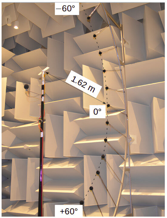
Figure 4.
ISAE-SUPAERO anechoic room and experimental setup.
The ideal rotor has a high FM to maximize the flight endurance and a low BPF SPL value to be acoustically stealthy. In the present paper, the optimization procedure relies on the following steps:
- The drone configuration and weight are defined, as well as the optimization design variables, space, and constraints. In the case of the present optimization, a quadcopter drone weighting ∼800 g is considered (meaning that each rotor must sustain approximately 2 N in hover).
- The multi-objective optimization is executed by using the NSGA-II optimization algorithm, the steady solver of the NVLM code (later called S-NLVM), and the Farassat formulation-1A [17] to predict the aerodynamic and aeroacoustic performance. Because of the concurrent nature of the two objectives, a set of all optimal solutions is obtained (hereafter referred to as the steady Pareto front, or steady PF).
- Three optimized rotors representing the Pareto front are chosen and tested using the unsteady solver of the NVLM code (or U-NVLM), and the “unsteady Pareto front” is obtained.
- The three rotors are then 3D-printed and experimentally tested in the anechoic room at ISAE-SUPAERO.
2.5. Optimization Setup
The optimization described in this paper takes into account multiple manufacturing constraints. The best geometries resulting from the optimization are 3D-printed using stereo-lithography techniques at ISAE-SUPAERO and tested in the anechoic room to verify the performance of the optimized geometries. The starting geometry of the following optimization is the 20 cm diameter rotor previously tested in the ISAE-SUPAERO anechoic room [9]. The rotor diameter was appositely chosen because it is the maximum diameter that could be 3D-printed in one piece with the available 3D-printer. For this study, only two-bladed rotors were tested because they are easier to balance statically. The NACA0012 aerodynamic coefficients calculated using XFOIL had previously been validated against experimental tests for different Reynolds numbers and angles of attack (as shown in [76]). This airfoil was therefore appropriately chosen to eliminate a possible source of discrepancy between the tests and the calculations when using lookup tables in the non-linear correction module embedded in the actual NVLM code. Its characteristics and the experimental results (evaluated at 2 N thrust) are summarized in Table 2.
Table 2.
Starting geometry parameters and performance. * Optimization variables.
All of the values in Table 2 are fixed throughout the optimization except for the chord and pitch distributions. That is, all tested rotors have two blades with a NACA0012 airfoil constant over the entire span of the blade and a diameter of 20 cm.
In order to minimize the number of parameters and still test very different rotor geometries, a blade reconstruction procedure previously introduced by the authors [82] is used. The optimization algorithm can select the parameter values within predefined minimum and maximum bounds using a continuous function. In this work, pitch and chord distributions are defined by three points: a point located at the root of the blade, one at the tip (called TIPx, where x is the parameter), and a control point (CPx, for which the spanwise position CPx,pos can be adjusted). The pitch and chord distributions are constructed as follows:
- The root pitch angle and chord length are set to 10° and 0.025 m, respectively;
- The CPpitch,pos defines the spanwise position at which the value CPpitch,ang is applied. The derivative of the curve at this point is fixed to zero (same strategy for the chord distribution with the CPchord,pos and CPchord,len variables, respectively);
- The pitch angle at the tip of the blade is defined by TIPpitch,ang (the chord length at the tip by TIPchord,len).
The BPoly.from_derivatives function of the Python (version 3.8.2) package Scipy version 1.4.1 [86] permits us to obtain the final distribution from the three different points by constructing a piecewise polynomial in the Bernstein basis. The parametrization used in this case has an advantage over conventional NURBS (non-uniform rational basis splines) because the interpolated curve always passes through the control points. This means that both the lower and upper bounds in the GA have a physical meaning. Figure 5 shows examples of pitch distribution interpolation.
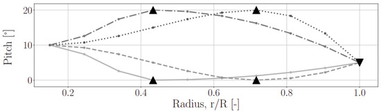
Figure 5.
Pitch distribution definition from the control point {CPpitch,pos, CPpitch,ang} (the upward pointing triangles) and the tip value TIPpitch,ang (the downward pointing triangles).
The total design space hence consists of six variables, presented in Table 3.
Table 3.
Design variables used in this part and their minimum and maximum bounds.
As this paper focuses on the performance of optimized 3D-printed rotors, multiple manufacturing and operational constraints are defined and set in the optimization to achieve robust and 3D-printable rotors. These constraints include limits on the chord length and solidity, due to the fact that rotors with higher solidities are generally heavier and more challenging to manufacture. The upper solidity limit was established to match that of the initial rotor design, while the lower limit was set at 0.08, a value that was arbitrarily chosen. Quadcopter drones are easily maneuverable due to their simplicity, as flight control is achieved by changing the rotational speed of the different rotors. However, the higher the inertia of the rotors, the more difficult it is to maneuver the drone. For this reason, an upper limit of inertia is fixed equal to the inertia of the starting geometry. For the rotational speed, because one critical structural mode of the test stand sustaining the rotor in the anechoic room is at around 3000 rpm, this value is selected as the lower limit.
The constraints (summarized in Table 4) are handled using a technique described by Deb et al. [81]. In an unconstrained single-objective optimization, when two solutions are compared, the one with the better objective value is chosen. In constrained multi-objective optimization, three different situations can be encountered: both solutions are feasible (i.e., they do not violate any constraints); one is feasible, and the other is not, and both violate the constraints. These three situations lead to different outcomes: the solution with the better objective value is chosen, the feasible solution is chosen, and the solution with smaller overall violation constraint is chosen, respectively. Taking into account solutions not feasible in the generation of a new offspring population is very important during the first generations, when the initial population is randomly chosen and the constraints are tight.
Table 4.
Constraints variables and lower/upper bounds.
In this study, each generation consists of 100 candidates randomly selected at the beginning. Both crossovers and mutations are activated with a probability of and , respectively, and the optimization stops after 50 generations.
3. Results
First, the results are presented in Section 3.1. The performance of the optimized geometries obtained with the S-NVLM/F1A code are then verified using U-NVLM/F1A simulations (in Section 3.2). The most interesting candidates are analyzed. In Section 3.3, the experimental aerodynamic and aeroacoustic results obtained in the anechoic room are discussed, and the performance of the optimization procedure is evaluated.
3.1. Optimization Convergence and Steady Pareto Fronts
During the optimization performed in this paper, a total of 5000 candidates were tested (100 candidates per generation × 50 generations). To check the convergence of the optimization, the moving averages of both objectives (FM and BPF SPL), obtained by averaging all the candidates satisfying the constraints and belonging to each generation, are plotted in Figure 6. The moving averages reach a plateau after ∼40 generations, indicating convergence.
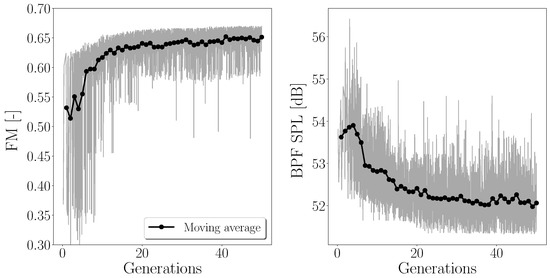
Figure 6.
Convergence plot showing the FM and the BPF SPL as functions of the generations. The dark dotted lines represent the moving average curves, while the grey lines represent the performance of all the simulated candidates.
Figure 7 shows the proportion of candidates that satisfy all the constraints of the optimization, as well as those that do not, plotted against the number of generations. Due to the random selection of the initial generation and the strict constraints, only 3 out of the 100 candidates meet all the criteria. After six generations, the rate of accepted candidates reaches 80% and remains constant until approximately the 30th generation, where it begins to decrease to a final rate of 60%. The results converge to the Pareto front, and the candidates are almost all borderline, with a solidity close to the maximum available value (as shown in Appendix B—Figure A2). Therefore, a small change in the chord can result in rejected candidates.
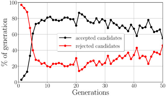
Figure 7.
Evolution of the number of rejected and accepted candidates per generation as functions of the generations.
Figure 8 illustrates the aerodynamic and aeroacoustic performance of all the candidates, including the last generation candidates. The ideal candidate should have the lowest BPF SPL and the highest FM, placing it in the bottom-right part of the graph. However, there is no single ideal candidate, but rather a set of optimized candidates belonging to the Pareto front (also called steady Pareto front). By following the Pareto front from right to left, the tonal noise is gradually reduced at the expense of the aerodynamic performance.

Figure 8.
Scatter plot showing all the candidates simulated, the last generation candidates and the Pareto front.
To assess the different contributions of both loading and thickness noise, the upper plots of Figure 9 show all the candidates colored by the thickness and loading noise components. The latter dominates the thickness noise, and it is therefore the main component of the tonal noise. It is also clear from the graph at the bottom left of Figure 9 that the tonal noise is linked to the rotational speed . To achieve the lowest possible BPF SPL, the nominal rotational speed is reduced. To do this, the rotor blades must develop higher thrust by increasing the chord towards the tip of the blade (increasing the rotor inertia, see bottom-right graph in Figure 9) and/or increasing the pitch value over the entire span of the blade (as previously described by the authors [82]) (avoiding stall). Note that reducing the rotational speed may not always decrease the tonal noise, especially if it causes significant changes in the relative contribution of the thickness noise to the overall tonal noise. The positions and values of the control points are presented in Appendix B.
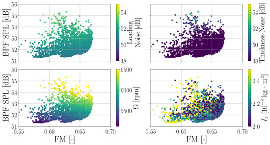
Figure 9.
Scatter plots showing the candidates colored by different variables: loading noise (top-left), thickness noise (top-right), nominal rotational speed (bottom-left), and rotor inertia (bottom-right).
To analyze the optimal solutions, three rotors representative of the full Pareto front were selected. Two geometries were chosen because they optimized one of the objectives. The rotor with the highest FM, called best aero rotor, and the rotor with the lowest tonal noise BPF SPL, that improves the BPF SPL by approximately 1.7 dB at a cost of 13% in FM compared to the best aero performance. However, as they did not optimize both objectives at the same time, another rotor with performance in-between was chosen, the compromise rotor. This final geometry reduces the noise by approximately 1.3 dB at a cost of 3% in FM compared to the best aero rotor.
These three geometries composing the steady Pareto front are shown in Figure 10, along with their chord and pitch distributions (the CAD models are shown in Figure 11).
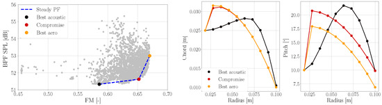
Figure 10.
On the left: scatter plot showing all the simulated candidates, three optimized rotors and the steady Pareto front. Chord (center) and pitch (right) distribution of the three optimized rotors belonging to the steady Pareto front.
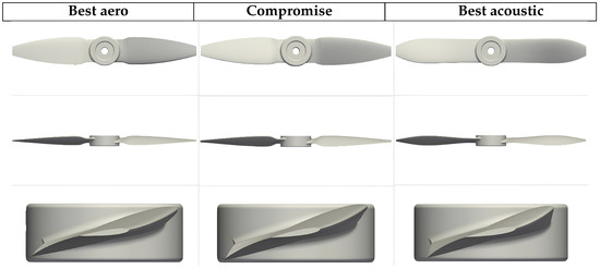
Figure 11.
The CAD models of the three optimized rotors.
While both best aero and best acoustic rotors have similar tip chords, the main difference lies in the control point. The best aero control point has a larger chord and is located close to the root. The best acoustic has a smaller chord at the control point, which is located outboard, resulting in a higher inertia (+). The pitch distributions are also significantly different between the two geometries. In the best aero geometry, the pitch control point is located near the root, at approximately the same position as the chord control point. However, it has a lower value than the best acoustic control point. Additionally, the pitch at the tip is also lower in the best aero rotor. These chord and pitch distributions enable the best acoustic rotor to produce greater thrust than the best aero rotor on the outer part of the blade. As a result, the rotational speed required to reach 2 N is lower than that of the best aero rotor (5170 rpm and 6212 rpm, respectively). Finally, the compromise geometry combines features of both rotors: it has a similar chord distribution to the best aero geometry, a similar pitch distribution shape, and it shares the same pitch value at the tip of the best acoustic blade. This design results in a performance that falls between the other two rotors. In summary, to slightly reduce the BPF tonal noise without affecting the aerodynamic efficiency of the rotor, it is advised to optimize the planform and the pitch distribution of the rotor, then adjust the collective pitch of the rotor blade. This will slow down the nominal rotational speed, resulting in quieter rotors. It is also worth mentioning that the chord and pitch distributions are neither linear nor hyperbolic near the tip. This is due to the particular geometric reconstruction based on the Bernstein basis polynomials, where the derivative of chord and pitch are set to zero in the control point (as discussed in Section 2.5). A different parametrization could have potentially led to linear/hyperbolic distributions near the tip.
3.2. Unsteady Pareto Front
Unsteady NVLM simulations were performed on steady Pareto front candidates. Two simulations per candidate are run to account for potential differences in thrust values resulting from higher fidelity simulations at the same rotational speed. The first simulation is run at the rotational speed predicted by the steady NVLM simulations (to reach the 2 N of thrust), while the second simulations is run at the rotational speed that satisfies the 2 N target thrust in U-NVLM simulations. The results are presented in Figure 12. Although the FM and BPF SPL have changed, the overall trend of the Pareto front remains unchanged, demonstrating the consistency between S-NVLM and U-NVLM simulations.

Figure 12.
Scatter plot showing the steady and unsteady (at iso rotational speed and 2 N iso thrust) Pareto fronts.
Unsteady simulations allow for a more accurate prediction of the rotor wake, and therefore, the analysis of the three different rotor wakes is performed on this basis. In the simulations, the rotor spins along the Z-axis and lies in the XY plane.
For all three optimized rotors, Figure 13 shows the instantaneous z-velocity () and vorticity magnitude () distributions after 10 rotations, while Figure 14 shows the z-velocity distributions averaged between the 10th and 15th rotations at four vertical positions in the Y = 0 plane.
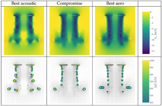
Figure 13.
Y = 0 planes colored by the instantaneous z-velocity (on top) and the vorticity magnitude (bottom) for the optimized rotors.
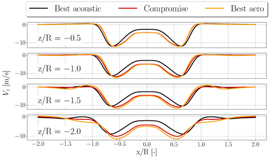
Figure 14.
Mean z-velocity distributions along radial position at different z locations for the three optimized rotors and at Y = 0 plane.
It can be observed that, for the best acoustic rotor, the induced velocities are stronger in the region close to the tip, where this rotor has larger chord lengths and pitch angles than the other two. This can be seen in Figure 13 and Figure 14, where a slightly less uniform z-velocity distribution is observed, with the highest induced velocities more concentrated at the tip compared to both compromise and best aero geometries. This phenomenon also leads to stronger tip vortices, and it is the reason for the higher values of vorticity magnitude observed for the best acoustic and compromise rotors compared to the best aero rotor (see Figure 14, bottom).
The tip vortices of the best acoustic configuration also tend to pair much earlier than the vortices of the other rotors, leading to earlier vortex merging. The location of the vortex merger trend is consistent with the findings of Ohanian et al. [87], where they showed that for rotors operating at comparable Reynolds numbers, the faster the rotor spins, the farther the vortex merger appears.
Figure 14 highlights the difference between the compromise and best aero rotors observed in Figure 13. While their z-velocity distributions are similar up to , the best aero rotor shows the most contracted wake of the three geometries from . This explains its higher efficiency (Froude’s theory shows that the ideal rotor has the highest contraction ratio, which can theoretically reach [78]).
The different pitch and chord distributions characterizing the optimized rotors also lead to different thrust and torque distributions (see Figure 15). When comparing the thrust distributions, it can be observed that the compromise and best aero rotors have the same thrust distribution. As the best acoustic rotor has larger pitch and chord values towards the tip of the blade, the thrust is more concentrated in this area. The location of the maximum thrust is located between 80% and 90% of the blade radius, and the thrust of the best acoustic blade is larger than the other two in this region, resulting in a center of thrust that is located at 75% of the rotor radius compared to 73% for the other two. While the thrust distribution is the same for the best aero and the compromise geometries, this is not the case for the torque distribution. The larger pitch values of the compromise blade induce larger torque over most of the blade span. The lower chord and pitch values of the best acoustic blade between the root and ∼55% of the radius induce lower torque values, while the opposite is observed outboard. The three centers of torque are located at 70% for the best aero, 71% for the compromise, and 75% for the best acoustic.
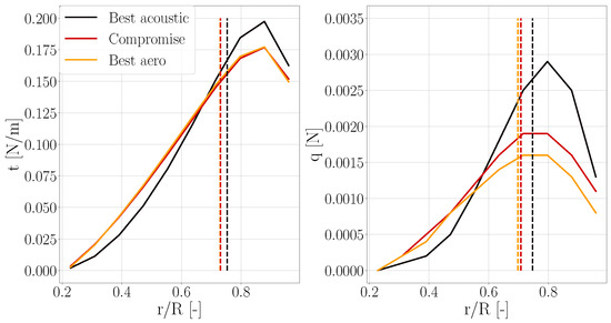
Figure 15.
Thrust and torque spanwise distribution (thrust per unit length t and torque per unit length q, respectively) of the three optimized rotors and their respective center of thrust and torque.
3.3. Experimental Analysis of Optimized Rotors
The CAD models of the three optimized rotors were created using the chord and pitch distributions generated by the optimization. For each rotor, the NACA0012 airfoil was 3D swept along the radial direction to create the 3D geometry of the blade which, in turn, was smoothly attached to the rotor hub.
The three optimized rotors were then 3D-printed in-house using Formlabs stereolithographic (SLA) 3D-printers [88], then polished with sandpaper and statically balanced. Note that the hand polishing process may introduce geometric differences between the CAD models (shown in Figure 11) and the final rotors. These differences are discussed in Appendix C.
Experimental tests were carried out in the ISAE-SUPAERO anechoic room to evaluate the aerodynamic performance and acoustic radiation of the three rotors at 1.62 m and angles ranging from −60° to 60°, where 0° corresponds to the plane of the rotor disk and positive angles are in the hemisphere containing the rotor wake (see Figure 4 and refer to Parisot-Dupuis et al. [89] for more details on the aerodynamic and acoustic setups). A 6-axis load cell was used to record the aerodynamic forces and moments. Only the averaged forces and moments along the z-axis are presented in Table 5, as they represent the rotor thrust (T) and torque (Q). An analysis of the uncertainties associated with these measurements is presented in Appendix A. For each rotor, the rotational speed was manually modified to achieve the target thrust of 2 N. As previously expected from both steady and unsteady simulations, the rotational speed required to achieve the target thrust increases from the best acoustic rotor to the compromise and best aero rotors. However, the ranking of FM and power () does not follow that of the simulations. While in the experiments the best acoustic rotor has the lowest efficiency (as expected), the compromise is the one with the highest FM, overtaking the best aero rotor by 3%, which is within the repeatability uncertainty.
Table 5.
Experimental aerodynamic results evaluated at ISA (international standard atmosphere) conditions: °C, , and .
Figure 16 shows the narrowband acoustic spectra of the three optimized rotors, recorded by the same microphone location used for the optimization (1.62 m from the rotor center and 30° below the rotor disk plane) at a sampling frequency of 51.2 kHz for 16 s.

Figure 16.
Experimental sound pressure level of the three optimized rotors taken from a microphone located 1.62 m from the rotor center and 30° below the rotor disk plane in the rotor wake direction.
The three spectra are composed of two distinct tonal peaks, one at the rotational frequency and one at the BPF, which are at least 10 dB higher than their harmonics, and a broadband noise whose shape varies greatly from one rotor to another.
The ranking of the BPF noise levels is the same as that predicted by the steady and unsteady Pareto fronts; although, in the experiments, the compromise BPF noise level is closer to the best acoustic one than predicted by the simulations. As mentioned above, the dominant component of the tonal noise for these 20 cm diameter rotors at 2 N thrust is the loading noise. Therefore, small changes in the geometry can induce different aerodynamic and aeroacoustic behavior (as shown by the change in the aerodynamic ranking). Furthermore, the 3D-printed blades are only statically balanced. This can explain the part of the spectra around 100 Hz of Figure 16, where tonal peaks at the rotational speeds are present and not negligible. The lowest rotational speed peak belongs to the compromise rotor, which seems to be the most dynamically balanced rotor of the three rotors tested. The tonal peaks have not been filtered out in the overall sound pressure level (OASPL) calculation, as they also affect the harmonics of the rotational speed.
While the trend of the tonal noise at the blade passing frequency is unchanged with respect to that found by simulation, the broadband noise from ∼110 Hz to 10 kHz shows an inverse trend. In this range, the best aero configuration is the one with the lowest broadband noise level. On the contrary, above 10 kHz, the high frequency broadband noise follows the tonal noise trend. However, it should be noted that the anechoic room allows free-field propagation up to 16 kHz. These results suggest that the optimization of the acoustic spectrum of low Reynolds number hovering rotors should include broadband noise when the minimization of the OASPL is the main objective. The mid-to-high frequency broadband noise is associated with turbulent and more complex phenomena that need to be simulated using semi-empirical models that relate the boundary layer properties and rotor geometry to the far-field acoustic radiation.
Both the tonal and broadband noise components of the MAV rotor have a certain directivity. It is therefore important to investigate the total directivity in order to fully assess the aeroacoustic performance. For this purpose, the directivity antenna shown in Figure 4 is used. The directivities of the BPF, the OASPL, which is obtained by integrating the entire acoustic spectrum from 80 Hz to 16 kHz (the range where the room is guaranteed to be anechoic), and the broadband noise (BBN), for which all the tonal peaks are filtered and the resulting spectrum is integrated from 1 kHz to 16 kHz, are shown in Figure 17.
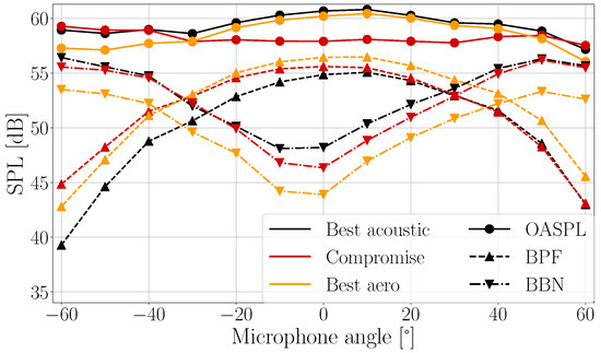
Figure 17.
Overall sound pressure level (OASPL), blade passing frequency (BPF), and broadband noise (BBN) directivities of the optimized rotors.
Between −30° and 30°, the BPF directivity follows the trend predicted by the simulations at the 30° microphone angle. Below −30°, the compromise geometry has the highest peaks and above 30° the lowest. The BPF maximum is at 10° for the best aero and the best acoustic, while it is at 0° for the compromise. As discussed in Section 3.1, the BPF SPL radiated by these rotors is mainly generated by the loading noise. It has been demonstrated [76] that its maximum moves towards positive microphone angles (i.e., downstream the rotor) when the torque decreases. As the BPF maximum of the best aero is at 10° and that of the compromise is at 0°, the trend is respected. However, the maximum at 10° for the best acoustic rotor does not seem to respect this theory. It should be noted that their geometries and operating rotational speeds are different, leading to different thrust and torque distributions and different centers of thrust and torque (see Figure 15), which may influence the radial position of the equivalent rotating dipole (please refer to Li Volsi [76] for more details).
The inverse trend in the BBN noise described above for the 30° microphone is confirmed for the other microphone angles and, as expected, the broadband noise level becomes more important than the BPF for microphone angles below −30° and above 30°. This again confirms that aeroacoustic optimizations should include the broadband noise in the optimization loop if the minimization of the OASPL is the objective. Since it is the result of the integration over the full acoustic spectrum, it can be considered as the sum of both tonal and broadband noise components. On the graph, it actually follows the BPF directivity trend between −30° and 30°, while it follows the trend of the broadband noise elsewhere, resulting in a different hierarchy to that obtained with the BPF SPL. However, there is an offset between the OASPL and the sum of the BBN and BPF, as the OASPL takes into account all the harmonics of the BPF and the peak at the rotational frequency (which are smoothed out in the BBN curve). If the OASPL had been the parameter to choose in this case, the compromise would have been the best candidate of the three tested, since it has the lowest levels from −30° to 40°, while the best acoustic rotor would have been the worst at almost all microphone angles.
In the light of the results discussed above, the experimental Pareto front is shown in Figure 18, together with both steady and unsteady Pareto fronts. While the aerodynamic and aeroacoustic performance of the best acoustic rotor are overestimated by the unsteady NVLM, the performance of the other two rotors are underestimated. The experimental tests also showed that the compromise rotor has the highest aerodynamic efficiency and a tonal noise very similar to that of the best acoustic rotor. However, these conclusions can be tempered by the ranges of uncertainties (described in Appendix A) and the comparisons between the CAD models of the scanned 3D-printed rotors and the initial geometries (presented in Appendix C). Comparing the experimental results of the three optimized rotors with the initial geometry (whose performance are summarized in Table 2), it can be concluded that the compromise and the best aero rotors improve the aerodynamic performance by more than (while the best acoustic has the same aerodynamic performance) and the acoustics BPF SPL by, at least, 4 dB. All the simulation and experimental results of the optimized rotors are summarized in Table 6.
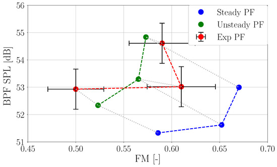
Figure 18.
Scatter plot showing the experimental Pareto front, as well as both simulated steady and unsteady Pareto fronts. Error bars are representing the uncertainty for a 95% confidence interval.
Table 6.
Summary of numerical and experimental results.
4. Conclusions and Perspectives
In this work, a multi-objective aeroacoustic optimization was performed using a steady non-linear vortex lattice method coupled with Farassat F1A acoustic analogy. The optimization was subject to manufacturing and operational constraints, such as the rotor inertia, its solidity and its rotational speed. The rotors were designed at 2 N iso-thrust, and the objectives were the aerodynamic efficiency (represented by the figure-of-merit) and the blade passing frequency sound pressure level (BPF SPL) for a microphone placed 30° below the rotor and at a far-field distance of 1.62 m. Pitch and chord distributions were modified by six design parameters. From the optimization, a set of optimized candidates (the steady Pareto front) was extracted, and three different optimized rotors were selected: one with the best aerodynamic performance, a second with the lowest blade passing frequency tonal noise, and a compromise. These three rotors were numerically tested using higher fidelity, unsteady non-linear vortex lattice method solver, and the unsteady Pareto front confirmed the trend predicted by the steady simulations. The analysis of the three wakes showed that the best aerodynamic rotor has the most contracted wake and an induced flow that is more homogeneous across the span of the blades. The best acoustic rotor, being the less aerodynamically efficient, had high induced velocities concentrated at the tip of the blade. This was combined with larger pitch angles at the tip to produce the same rotor thrust at lower rotational speeds than the other rotors, thus reducing the BPF acoustic footprint of the rotor. The compromise, with a similar chord distribution but slightly larger pitch angles than the best aerodynamic rotor, rotates slower than the best aerodynamic rotor and has similar wake characteristics. The optimized rotors were then 3D-printed, hand-polished, statically balanced, and tested in the ISAE-SUPAERO anechoic room. A microphone directivity antenna and a load cell were used to evaluate the aerodynamic and acoustic performance used for the optimization. The compromise rotor has the best aerodynamic efficiency and a tonal noise level close to the best acoustic rotor. However, the best acoustic rotor is the geometry showing the highest broadband noise and overall sound pressure level. While the difference in the aerodynamic trend is within the experimental uncertainty, the broadband noise shows a clear and inverse trend. To optimize the full acoustic spectrum using different criteria, such as Overall Sound Pressure Level (OASPL) or A-weighted OASPL, it is necessary to include both brandband and tonal noise at the blade passing frequency in the optimization loop.
Author Contributions
Conceptualization, P.L.V., T.J. and R.G.; methodology, P.L.V., T.J., R.G. and H.P.-D.; software, P.L.V.; validation, P.L.V., T.J., R.G. and H.P.-D.; formal analysis, P.L.V., T.J., R.G. and H.P.-D.; investigation, P.L.V., T.J., R.G. and H.P.-D.; resources, G.B.; data curation, P.L.V.; writing—original draft preparation, P.L.V.; writing—review and editing, P.L.V., T.J., R.G., G.B. and H.P.-D.; visualization, P.L.V. and H.P.-D.; supervision, P.L.V., T.J. and R.G.; project administration, T.J., R.G. and J.-M.M.; funding acquisition, J.-M.M. All authors have read and agreed to the published version of the manuscript.
Funding
This work has been financed by Parrot Drones SAS and the Association Nationale Recherche Technologie (ANRT) under grant CIFRE N°2019/1072, realized at ISAE-SUPAERO and performed using HPC resources from PANDO (ISAE-SUPAERO), and GENCI [CCRT-CINES-IDRIS] (Grant 2022-[A0122A07178] and 2023-[A0142A07178]).
Data Availability Statement
The raw data supporting the conclusions of this article will be made available by the authors on request.
Acknowledgments
The authors express their gratitude to Sylvain Belliot and Bertrand Mellot for their technical assistance in printing and testing the optimized rotors. Additionally, Chakshu Deorra provided valuable support in the use of the 3D scanner. We acknowledge that the use of large language models (https://chat.openai.com/ [accessed on 23 February 2024] and https://www.deepl.com/write [accessed on 23 February 2024]) was strictly limited to correcting grammatical and syntax errors in the final editing and proofreading phase of the manuscript.
Conflicts of Interest
Romain Gojon, Thierry Jardin, Hélène Parisot-Dupuis, Jean-Marc Moschetta declare no conflicts of interest. Pietro Li Volsi and Gianluigi Brogna were employees of Parrot Drones SAS during the execution of the research presented in the article.
Abbreviations
The following abbreviations are used in this manuscript:
| BBN | Broadband noise |
| BEMT | Blade element momentum theory |
| BPF | Blade passing frequency |
| BVI | Blade vortex interaction |
| CAD | Computer-aided design |
| CFD | Computational fluid dynamics |
| CP | Control point |
| DNS | Direct numerical simulation |
| DOE | Design of experiments |
| DRE | Data reduction equation |
| F1A | Farassat formulation 1A |
| FM | Figure-of-merit |
| FFT | Fast-Fourier transform |
| FW-H | Ffowcs Williams and Hawkings |
| GA | Genetic algorithm |
| HK | Hierarchical kriging |
| LES | Large eddy simulation |
| LIDAR | Laser imaging detection and ranging |
| MAV | Micro air vehicle |
| MCM | Monte Carlo method |
| NSGA | Non-dominated sorting genetic algorithm |
| NURBS | Non-uniform rational basis splines |
| NVLM | Non-linear vortex lattice method |
| OASPL | Overall sound pressure level |
| PDS | Penetrable data surface |
| PF | Pareto front |
| RANS | Reynolds-averaged Navier–Stokes simulation |
| RPM | Revolutions per minute |
| S-NVLM | Steady non-linear vortex lattice method |
| SLA | Stereolithography |
| SPL | Sound pressure level |
| TSM | Taylor series method |
| U-NVLM | Unsteady non-linear vortex lattice method |
| VLM | Vortex lattice method |
| VPM | Vortex particle method |
Appendix A. Uncertainty Analysis
In order to improve the comparison between numerical and experimental results, an uncertainty analysis of the measurements has been performed. On steady-state experiments like the measurement of the figure of merit (FM) of an isolated rotor, errors can be induced by
- Calibration errors;
- Variations of atmospheric conditions (temperature, humidity, ambient pressure, etc.);
- Unsteadiness in measurements.
In the ISO 1993 GUM guide issued in 1993 [90], two different types of uncertainties are defined: the type A uncertainty, which is calculated by statistical analysis of series of observations, and type B uncertainty calculated by other means than the statistical analysis. Uncertainties () on measured variables [91] are calculated from the root-sum-square (RSS) of the random standard uncertainty, , and the systematic standard uncertainties, (b for bias):
Once the uncertainty for a measured variable (X) is obtained, it is important to “expand” this uncertainty with an associated level of confidence. In this work, a level of confidence of is chosen. To calculate the expanded uncertainty , the following equation is needed:
where depends on the degree of freedom (DOF) of the sample population.
As expressed before, one of the results analyzed here in the work is the figure of merit (FM), whose equation is defined in Equation (7). This quantity, being the result of a data reduction equation (DRE), is not a directly measurable variable. When it comes to calculating the uncertainty of a DRE result (r), all the uncertainties affecting the measured quantities must be taken into account. It is possible to do so by using two different approaches: the Monte Carlo method (MCM) and the Taylor series method (TSM) [92]. Here, the TSM method is used and the combined standard uncertainty in the dimensionless form is presented, by considering .
where
- is the relative uncertainty;
- is the uncertainty magnification factor. If it is greater than one, then its uncertainty will have bigger repercussions on the combined uncertainty.
When applying Equation (A3) for the calculation of the FM uncertainty,
Since the air density () is also a result of a DRE, the equation associated should be taken into account and its value is injected in Equation (A4):
The uncertainty on the gaz constant () is considered equal to zero. The calculation of the FM uncertainty was carried out beforehand by running (and taking into account only) a repeatability test on the reference rotor described in Table 2 at 5000 RPM. In total, 19 measurements were collected and both mean and standard deviation values of all the measured variables are shown in Table A1.
Table A1.
Repeatability measured variables uncertainties.
Table A1.
Repeatability measured variables uncertainties.
| Results | T [N] | Q [Nmm] | [RPM] | p [Pa] | T [K] | [kg/m3] | BPF SPL [dB] |
|---|---|---|---|---|---|---|---|
| 0.940 | 12.110 | 4999.41 | 99,731.27 | 292.08 | 1.189541 | 45.96 | |
| 0.016 | 0.115 | 0.18 | 2.74 | 0.03 | 0.000094 | 0.35 |
Since this repeatability test uses the same blade, there is no calculable standard deviation on the radius (R) of the rotor. This led to the following relative, absolute, and expanded uncertainties on the FM on which the error-bars are based in Figure 18:
Since the BPF SPL is the result of only one measured variable, its uncertainty depends only on the standard deviation of the repeatability test:
Appendix B. Constrained Optimization-Design Variables and Constraints
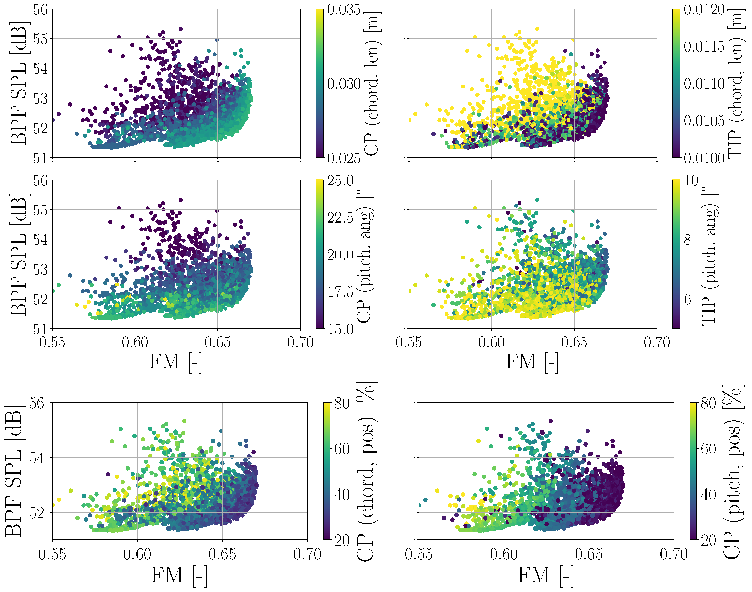
The distribution of the six design variables used for the constrained optimization discussed in Section 3 is shown in Figure A1: the chord control point and tip lengths (CPchord,len at top-left and TIPchord,len at top-right, respectively), the pitch control point and tip angles (CPpitch,ang at center-left and TIPpitch,ang at center-right), and the spanwise relative position of the chord and pitch control points (CPchord,pos at bottom-left and CPpitch,pos at bottom-right).
Because of the solidity and inertia constraints, the position of the chord control point CPchord,pos and its value CPchord,len change within the Pareto front. For silent rotors, CPchord,pos, and their value CPchord,len is relatively low compared to the more aerodynamically efficient rotors to avoid an increase in the inertia and to decrease the rotational speed. More aerodynamically efficient rotors, on the other hand, have larger chords at the control point and its position is relatively close to the hub. The values of the tip chord are quite similar for all Pareto front candidates.
Higher pitch angles on both control point CPpitch,ang and tip TIPpitch,ang are used to reduce the rotational speed and the tonal noise. Moreover, the position of the pitch control point CPpitch,pos is located at 70% of the rotor radius to help in reducing the nominal speed of the rotor.
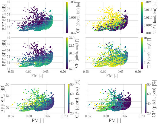
Figure A1.
Scatter plots showing the candidates colored by different variables: CPchord,len (top-left), TIPchord,len (top-right), CPpitch,ang (center-left), TIPpitch,ang (center-right), CPchord,pos (bottom-left), CPpitch,pos (bottom-right).
Figure A1.
Scatter plots showing the candidates colored by different variables: CPchord,len (top-left), TIPchord,len (top-right), CPpitch,ang (center-left), TIPpitch,ang (center-right), CPchord,pos (bottom-left), CPpitch,pos (bottom-right).
The distribution of the rotor solidity is shown in Figure A2. All the Pareto front candidates reach larger solidities (approaching the maximum allowed solidity ), when compared to the other candidates. The large solidity of the Pareto front candidates next to the best aero rotor is caused by larger control point chords, while the ones next to the best acoustic rotor have larger tip chords.
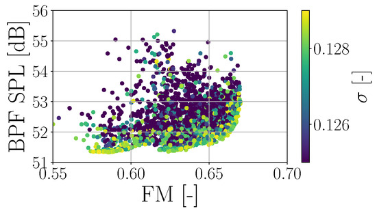
Figure A2.
Scatter plot showing the candidates colored by the rotor solidity .
Figure A2.
Scatter plot showing the candidates colored by the rotor solidity .
Appendix C. Comparison between CAD Models and 3D-Printed Rotors
The discrepancy between predictions made by U-NVLM and S-NVLM simulations and the results of experimental tests on the compromise rotor have prompted the analysis of 3D-printed rotors and their comparison to the CAD models used to print the rotors. With this goal in mind, the scanner Solutionix C500 [93] is used. Figure A3 shows the setup including one of the optimized rotors that have been scanned. This scanner utilizes a laser, two cameras, and the phase-shifting optical triangulation process to create 3D models of objects. A turning table permits to rotate the object around three different axes to capture all the object surfaces.
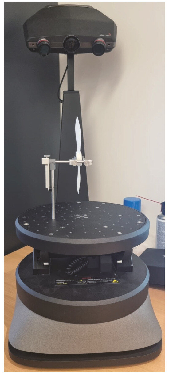
Figure A3.
Setup of the Solutionix C500 scanner with the rotor mounted on the turntable.
Figure A3.
Setup of the Solutionix C500 scanner with the rotor mounted on the turntable.
The optimized rotors have a diameter of 20 cm, which necessitates a camera with a field of view of 500 mm, for this scanner. This enables the scanning of objects up to 385 mm × 312 mm × 210 mm. Once the scanner acquires point clouds at different orientations, the software reconstructs the full geometry, that is then exported in STL format. This allows us to compare it with the original CAD model (in the same format). Global comparisons between CAD models and scanned STLs are performed on Paraview [94]. Geomagic Design X [95] is then used to perform point-to-point comparisons of two geometries, determining the distance in millimeters between two surfaces (suction or pressure side surfaces), as well as calculating and comparing the local thickness of the geometries. For each rotor, Paraview and Geomagic comparisons are presented:
- best aero rotor: Figure A4 shows small differences between the CAD and scanned models, with the tip of the scanned model slightly bent upward. Colormaps of Figure A5 confirm the small deflection at the tip, with differences reaching 1.2 mm. The thickness comparison shows differences smaller than 0.1 mm. The squared patches on thickness and suction side figures are caused by the reflective patch used to measure the rotational speed.
- best acoustic rotor: The tips of the scanned blades resulted bent downward when compared to the CAD model. Point-to-point distances between the suction and pressure sides of CAD/scanned models showed a spanwise gradient, with a difference reaching 1.6 mm. Small differences in the pitch distribution were visualized by chordwise gradients, visible on both suction and pressure sides. The thickness differences showed good agreements between the CAD and printed rotors.
- compromise rotor: Bigger differences (when compared to the best aero and compromise rotors) are measured at the tip of the blades, as the scanned blades result bent upward. The point-to-point distances between the suction and pressure sides of CAD/scanned models showed spanwise and chordwise gradients, with a maximum difference reaching 4.3 mm at the tip. The thickness differences are also bigger than the other rotors, reaching 0.6 mm.
The results reported above confirm that the printed compromise rotor presents the biggest differences with its original CAD model. Attention must be paid on the values obtained with Geomagic, since the automatic rotation of the 3D-scanned rotor reference system to the CAD model is sometimes not perfect and needs manual corrections. However, visualizations performed on Paraview permit to confirm the trends predicted by Geomagic.
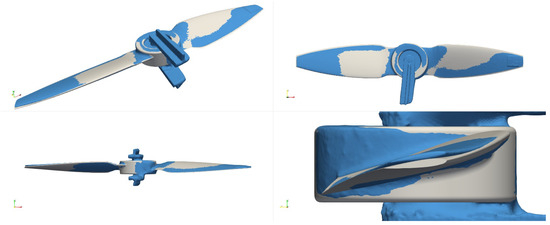
Figure A4.
best aero CAD (gray) and 3D-scanned (light blue) models comparisons.
Figure A4.
best aero CAD (gray) and 3D-scanned (light blue) models comparisons.

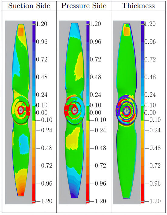
Figure A5.
best aero Comparison of suction side (the scale goes from −1.2 mm to 1.2 mm), pressure side (−1.2 mm to 1.2 mm) and thickness (−1.2 mm to 1.2 mm).
Figure A5.
best aero Comparison of suction side (the scale goes from −1.2 mm to 1.2 mm), pressure side (−1.2 mm to 1.2 mm) and thickness (−1.2 mm to 1.2 mm).

References
- Custers, B. Drones Here, There and Everywhere Introduction and Overview. In The Future of Drone Use: Opportunities and Threats from Ethical and Legal Perspectives; Custers, B., Ed.; T.M.C. Asser Press: The Hague, The Netherlands, 2016; pp. 3–20. [Google Scholar] [CrossRef]
- Frachtenberg, E. Practical Drone Delivery. Computer 2019, 52, 53–57. [Google Scholar] [CrossRef]
- Eisenbeiss, H. UAV Photogrammetry. Doctoral Thesis, ETH Zurich, Zürich, Switzerland, 2009. [Google Scholar] [CrossRef]
- Kardasz, P.; Doskocz, J. Drones and Possibilities of Their Using. J. Civ. Environ. Eng. 2016, 6, 233. [Google Scholar] [CrossRef]
- Alvarado, E. 237 Ways Drone Applications Revolutionize Business. Drone Ind. Insights 2021, 540. Available online: https://droneii.com/237-ways-drone-applications-revolutionize-business (accessed on 23 February 2024).
- Alvarado, E. What are the top drone applications? Drone Ind. Insights 2022. Available online: https://droneii.com/top-drone-applications (accessed on 23 February 2024).
- Jones, T.M. International Commercial Drone Regulation and Drone Delivery Services; RAND Corporation: Santa Monica, CA, USA, 2017. [Google Scholar] [CrossRef]
- Lee, H.; Lee, D.J. Rotor interactional effects on aerodynamic and noise characteristics of a small multirotor unmanned aerial vehicle. Phys. Fluids 2020, 32, 047107. [Google Scholar] [CrossRef]
- Gojon, R.; Doué, N.; Parisot-Dupuis, H.; Mellot, B.; Jardin, T. Aeroacoustic radiation of a low Reynolds number two-bladed rotor in interaction with a cylindrical beam. In Proceedings of the 28th AIAA/CEAS Aeroacoustics 2022 Conference, Southampton, UK, 14–17 June 2022. [Google Scholar] [CrossRef]
- Zarri, A.; Dell’Erba, E.; Schram, C.F. Fuselage scattering effects in a hovering quadcopter drone. In Proceedings of the 28th AIAA/CEAS Aeroacoustics 2022 Conference, Southampton, UK, 14–17 June 2022. [Google Scholar] [CrossRef]
- Zawodny, N.S.; Boyd, D.D. Investigation of RotorAirframe Interaction Noise Associated with Small-Scale Rotary-Wing Unmanned Aircraft Systems. J. Am. Helicopter Soc. 2020, 65, 1–17. [Google Scholar] [CrossRef]
- Schäffer, B.; Pieren, R.; Heutschi, K.; Wunderli, J.M.; Becker, S. Drone noise emission characteristics and noise effects on humans—A systematic review. Int. J. Environ. Res. Public Health 2021, 18, 5940. [Google Scholar] [CrossRef]
- Burley, C.L.; Brooks, T.F. Rotor Broadband Noise Prediction with Comparison to Model Data. J. Am. Helicopter Soc. 2004, 49, 28–42. [Google Scholar] [CrossRef]
- Gutin, L. On the sound field of a rotating airscrew. Zhurnal Tekhnicheskoi Fiz. 1936, 6, 899–909. [Google Scholar]
- Ernsthausen, W. The Source of Propeller Noise. NACA-TM-825, 6 September 2013. NACA Technical Memorandum. Available online: https://ntrs.nasa.gov/citations/19930094591 (accessed on 23 February 2024).
- Deming, A.F. Noise from Propellers with Symmetrical Sections at Zero Blade Angle, II. NACA Technical Note. NACA-TN-679, 6 September 2013. Available online: https://ntrs.nasa.gov/citations/19930081438 (accessed on 23 February 2024).
- Farassat, F.; Succi, G.P. The Prediction of Helicopter Discrete Frequency Noise. Vertica 1983, 7, 309–320. [Google Scholar]
- Ffowcs Williams, J.E.; Hawkings, D.L.; Lighthill, M.J. Sound generation by turbulence and surfaces in arbitrary motion. Philos. Trans. R. Soc. London. Ser. A Math. Phys. Sci. 1969, 264, 321–342. [Google Scholar] [CrossRef]
- Jo, Y.; Jardin, T.; Gojon, R.; Jacob, M.C.; Moschetta, J.M. Prediction of noise from low Reynolds number rotors with different number of blades using a non-linear vortex lattice method. In Proceedings of the 25th AIAA/CEAS Aeroacoustics Conference, Delft, The Netherlands, 20–23 May 2019; p. 2615. [Google Scholar] [CrossRef]
- Li Volsi, P.; Jardin, T.; Gojon, R.; Gomez-Ariza, D.; Moschetta, J.M.; Parisot-Dupuis, H.; Brogna, G. Aerodynamic and Aeroacoustic Study of Low Reynolds Number Rotors: Influence of Pitch Angle, Airfoil Camber and Thickness. In Proceedings of the 28th AIAA/CEAS Aeroacoustics 2022 Conference, Southampton, UK, 14–17 June 2022. [Google Scholar] [CrossRef]
- Williams, J.E.F.; Hall, L.H. Aerodynamic sound generation by turbulent flow in the vicinity of a scattering half plane. J. Fluid Mech. 1970, 40, 657–670. [Google Scholar] [CrossRef]
- Amiet, R.K. Noise due to turbulent flow past a trailing edge. J. Sound Vib. 1976, 47, 387–393. [Google Scholar] [CrossRef]
- Amiet, R.K. Acoustic radiation from an airfoil in a turbulent stream. J. Sound Vib. 1975, 41, 407–420. [Google Scholar] [CrossRef]
- Roger, M.; Moreau, S. Back-scattering correction and further extensions of Amiet’s trailing-edge noise model. Part 1: Theory. J. Sound Vib. 2005, 286, 477–506. [Google Scholar] [CrossRef]
- Moreau, S.; Roger, M. Back-scattering correction and further extensions of Amiet’s trailing-edge noise model. Part II: Application. J. Sound Vib. 2009, 323, 397–425. [Google Scholar] [CrossRef]
- Roger, M.; Moreau, S. Addendum to the back-scattering correction of Amiet’s trailing-edge noise model. J. Sound Vib. 2012, 331, 5383–5385. [Google Scholar] [CrossRef]
- Brooks, T.; Pope, D.; Marcolini, M. Airfoil Self-Noise and Prediction; Technical Report NASA Reference Publication 1218; National Aeronautics and Space Administration: Washington, DC, USA, 1989. Available online: https://ntrs.nasa.gov/api/citations/19890016302/downloads/19890016302.pdf (accessed on 23 February 2024).
- Gan, Z.F.; Brentner, K.S.; Greenwood, E. Time Variation of Helicopter Rotor Broadband Noise. In Proceedings of the 28th AIAA/CEAS Aeroacoustics 2022 Conference, Southampton, UK, 14–17 June 2022. [Google Scholar] [CrossRef]
- Li, S.K.; Lee, S. Prediction of Rotorcraft Broadband Trailing-Edge Noise and Parameter Sensitivity Study. J. Am. Helicopter Soc. 2020, 65, 1–14. [Google Scholar] [CrossRef]
- Roger, M.; Moreau, S.; Guedel, A. Broadband fan noise prediction using single-airfoil theory. Noise Control. Eng. J. 2006, 54, 5–14. [Google Scholar] [CrossRef]
- Moreau, S.; Roger, M. Competing broadband noise mechanisms in low-speed axial fans. AIAA J. 2007, 45, 48–57. [Google Scholar] [CrossRef]
- Sanjosé, M.; Moreau, S. Fast and accurate analytical modeling of broadband noise for a low-speed fan. J. Acoust. Soc. Am. 2018, 143, 3103–3113. [Google Scholar] [CrossRef]
- Zarri, A. Aerodynamic and Acoustic Investigation of Automotive Fan-Driven Cooling Systems. Ph.D. Thesis, Université de Lyon, Rhode-Saint-Genèse, Belgique, 2021. [Google Scholar]
- Tian, Y.; Cotté, B. Wind turbine noise modeling based on Amiet’s theory: Effects of wind shear and atmospheric turbulence. Acta Acust. United Acust. 2016, 102, 626–639. [Google Scholar] [CrossRef]
- Cotté, B. Extended source models for wind turbine noise propagation. J. Acoust. Soc. Am. 2019, 145, 1363–1371. [Google Scholar] [CrossRef]
- Cotté, B.; Mascarenhas, D.; Roy, S.; Doaré, O. Wind turbine noise auralization including tonal and broadband aeroacoustic sources. In Proceedings of the 10th Convention of the European Acoustics Association Forum Acusticum 2023, Torino, Italy, 11–15 September 2023; pp. 5455–5458. [Google Scholar] [CrossRef]
- Bhargava Nukala, V.; Prasad Padhy, C. Concise review: Aerodynamic noise prediction methods and mechanisms for wind turbines. Int. J. Sustain. Energy 2023, 42, 128–151. [Google Scholar] [CrossRef]
- Mueller, T.J.; DeLaurier, J.D. Aerodynamics of small vehicles. Annu. Rev. Fluid Mech. 2003, 35, 89–111. [Google Scholar] [CrossRef]
- Grande, E.; Ragni, D.; Avallone, F.; Casalino, D. Laminar Separation Bubble Noise on a Propeller Operating at Low Reynolds Numbers. AIAA J. 2022, 60, 5324–5335. [Google Scholar] [CrossRef]
- Jaroslawski, T.; Forte, M.; Moschetta, J.M.; Delattre, G.; Gowree, E.R. Characterisation of boundary layer transition over a low Reynolds number rotor. Exp. Therm. Fluid Sci. 2022, 130, 110485. [Google Scholar] [CrossRef]
- Gojon, R.; Jardin, T.; Parisot-Dupuis, H. Experimental investigation of low Reynolds number rotor noise. J. Acoust. Soc. Am. 2021, 149, 3813–3829. [Google Scholar] [CrossRef] [PubMed]
- Lissaman, P.B.S. Low-Reynolds-Number Airfoils. Annu. Rev. Fluid Mech. 1983, 15, 223–239. [Google Scholar] [CrossRef]
- Winslow, J.; Otsuka, H.; Govindarajan, B.; Chopra, I. Basic understanding of airfoil characteristics at low Reynolds numbers (104–105). J. Aircr. 2018, 55, 1050–1061. [Google Scholar] [CrossRef]
- Vogeley, A.W. Sound-Level Measurements of a Light Airplane Modified to Reduce Noise Reaching the Ground; Technical Report; National Advisory Committee for Aeronautics: Washington, DC, USA, 1949. [Google Scholar]
- Demory, B.; Henner, M.; Levasseur, A.; Moreau, S.; Motors, V. Optimized Efficient Quiet Automotive Fan Systems. In Proceedings of the International Congress Fluid Dynamics Applications in Ground Transportation, Lyon, France, 26–27 October 2005. [Google Scholar]
- Kim, J.-S.; Jeong, U.C.; Kim, D.W.; Han, S.Y.; Oh, J.E. Optimization of sirocco fan blade to reduce noise of air purifier using a metamodel and evolutionary algorithm. Appl. Acoust. 2015, 89, 254–266. [Google Scholar] [CrossRef]
- Jaron, R.; Moreau, A.; Guérin, S.; Enghardt, L.; Lengyel-Kampmann, T.; Otten, T.; Nicke, E. Multidisciplinary Design Optimization of a Low-Noise and Efficient Next-Generation Aero-Engine Fan. J. Turbomach. 2021, 144, 011004. [Google Scholar] [CrossRef]
- Succi, G.P. Design of quiet efficient propellers. SAE Tech. Pap. 1979, 88, 2039–2052. [Google Scholar] [CrossRef]
- Howard, P.; Ronald, F.; Chandra, S.; Howard, P.; Ronald, F.; Chandra, S. Two and three-bladed propeller design for the reduction of radiated noise. In Proceedings of the 3rd AIAA/CEAS Aeroacoustics Conference, Atlanta, GA, USA, 12–14 May 1997. [Google Scholar] [CrossRef]
- Pagano, A.; Barbarino, M.; Casalino, D.; Federico, L. Tonal and broadband noise calculations for aeroacoustic optimization of a pusher propeller. J. Aircr. 2010, 47, 835–848. [Google Scholar] [CrossRef]
- Marinus, B.; Roger, M.; Van Den Braembussche, R. Aeroacoustic and Aerodynamic Optimization of Aircraft Propeller Blades. In Proceedings of the 16th AIAA/CEAS Aeroacoustics Conference, Stockholm, Sweden, 7–9 June 2010. [Google Scholar] [CrossRef]
- Marinus, B.; Roger, M.; Van Den Braembussche, R.; Bosschaerts, W. Multidisciplinary Optimization of Propeller Blades: Focus on the aeroacoustic results. In Proceedings of the 17th AIAA/CEAS Aeroacoustics Conference (32nd AIAA Aeroacoustics Conference), Portland, Oregon, 5–8 June 2011. [Google Scholar] [CrossRef]
- Kotwicz Herniczek, M.T.; Feszty, D.; Meslioui, S.A.; Park, J. Applicability of early acoustic theory for modern propeller design. In Proceedings of the 23rd AIAA/CEAS Aeroacoustics Conference, Denver, CO, USA, 5–9 June 2017; pp. 1–19. [Google Scholar] [CrossRef]
- Huang, Z.J.; Yao, H.D.; Lundbladh, A.; Davidson, L. Low-Noise Propeller Design for Quiet Electric Aircraft. In Proceedings of the AIAA Aviation 2020 Forum, Virtual Event, 15–19 June 2020. [Google Scholar] [CrossRef]
- Yu, P.; Peng, J.; Bai, J.; Han, X.; Song, X. Aeroacoustic and aerodynamic optimization of propeller blades. Chin. J. Aeronaut. 2020, 33, 826–839. [Google Scholar] [CrossRef]
- Barbarino, M.; Pagano, A.; Quagliarella, D.; Visingardi, A.; Bernardini, G.; Gennaretti, M.; Poggi, C. VENUS D2.2: Aerodynamic and Aeroacoustic Design and Optimization of the New Aircraft DEP Configuration. Project Deliverable, CIRA and University of RomaTre. Delivered May 2021. Grant Agreement No. 886019. Available online: https://venus.ing.uniroma3.it (accessed on 11 April 2024).
- Pagano, A.; Federico, L.; Barbarino, M.; Guida, F.; Aversano, M. Multi-Objective Aeroacoustic Optimization of an Aircraft Propeller. In Proceedings of the 12th AIAA/ISSMO Multidisciplinary Analysis and Optimization Conference, Victoria, BC, Canada, 10–12 September 2008. [Google Scholar] [CrossRef]
- Wilke, G. Quieter and Greener rotorcraft: Concurrent aerodynamic and acoustic optimization. CEAS Aeronaut. J. 2021, 12, 495–508. [Google Scholar] [CrossRef]
- Wilke, G. Findings in Aero-Acoustic Simulations for Optimizations. In Proceedings of the 76th Annual Forum, Virtual, 5–8 October 2020. [Google Scholar]
- Zhou, Z.; Huang, J.; Yi, M. Comprehensive optimization of aerodynamic noise and radar stealth for helicopter rotor based on Pareto solution. Aerosp. Sci. Technol. 2018, 82–83, 607–619. [Google Scholar] [CrossRef]
- Bu, Y.; Song, W.; Han, Z.; Zhang, Y.; Zhang, L. Aerodynamic/aeroacoustic variable-fidelity optimization of helicopter rotor based on hierarchical Kriging model. Chin. J. Aeronaut. 2020, 33, 476–492. [Google Scholar] [CrossRef]
- Yang, C.; Aoyama, T.; Chae, S.; Yee, K.; Jeong, S.; Obayashi, S. Blade planform optimization to reduce HSI noise of helicopter in hover. Annu. Forum Proc.-Ahs Int. 2008, 3, 2218–2232. [Google Scholar]
- Polyzos, N.D.; Vouros, S.; Goulos, I.; Pachidis, V. Multi-disciplinary optimization of variable rotor speed and active blade twist rotorcraft: Trade-off between noise and emissions. Aerosp. Sci. Technol. 2020, 107, 106356. [Google Scholar] [CrossRef]
- Gur, O.; Rosen, A. Design of a quiet propeller for an electric mini unmanned air vehicle. J. Propuls. Power 2009, 25, 717–728. [Google Scholar] [CrossRef]
- Wisniewski, C.F.; Byerley, A.R.; Heiser, W.H.; Van Treuren, K.W.; Liller, W.R. Designing small propellers for optimum efficiency and low noise footprint. In Proceedings of the 33rd AIAA Applied Aerodynamics Conference, Dallas, TX, USA, 22–26 June 2015; pp. 1–17. [Google Scholar] [CrossRef]
- Boyer, F.; Drapier, A.M.; Mérillac, Y.; Nana, C. Multidisciplinary optimization of a MAV propeller for noise reduction. In Proceedings of the International Micro Air Vehicle Conference, Toulouse, France, 18–21 September 2017; pp. 301–306. [Google Scholar]
- Serré, R.; Gourdain, N.; Jardin, T.; Jacob, M.C.; Moschetta, J.M. Towards silent micro-air vehicles: Optimization of a low Reynolds number rotor in hover. Int. J. Aeroacoust. 2019, 18, 690–710. [Google Scholar] [CrossRef]
- Gur, O.; Silver, J.; Dítě, R.; Sundhar, R. Optimized Performance and Acoustic Design of Hover-Propeller. In Proceedings of the AIAA Aviation and Aeronautics Forum and Exposition, AIAA AVIATION Forum 2021, Virtual Event, 2–6 August 2021. [Google Scholar] [CrossRef]
- Pullin, S.F.; Zhou, B.Y.; Azarpeyvand, M. Optimisation of Propellers with Noise-Based Constraints Including a Deep Learning Method for Aerofoil Prediction. In Proceedings of the 28th AIAA/CEAS Aeroacoustics 2022 Conference, Southampton, UK, 14–17 June 2022. [Google Scholar] [CrossRef]
- Klimczyk, W.; Sieradzki, A. RANS-Based Aeroacoustic Global Sensitivity Study and Optimization of UAV Propellers. Aerospace 2023, 10, 306. [Google Scholar] [CrossRef]
- Sarikaya, B.; Zarri, A.; Christophe, J.; Aissa, M.; Verstraete, T.; Schram, C. Aerodynamic and Aeroacoustic Design Optimization of UAVs Using a Surrogate Model. 2023. Available online: https://ssrn.com/abstract=4679895 (accessed on 22 February 2024).
- Gessow, A. Effect of Rotor-Blade Twist and Plan-Form Taper on Helicopter Hovering Performance; Technical Report; NACA: Washington, DC, USA, 1948. [Google Scholar]
- Jo, Y.; Lee, H.; Lee, D.J. Prediction of rotor flow for unmanned aerial system using nonlinear vortex lattice method. In Proceedings of the 6th Asia/Australian Rotorcraft Forum/Heli Japan, Kanazawa, Japan, 7–9 November 2017. [Google Scholar]
- Katz, J.; Plotkin, A. Low-Speed Aerodynamics; Cambridge University Press: Cambridge, UK, 2001. [Google Scholar]
- Drela, M. XFOIL: An Analysis and Design System for Low Reynolds Number Airfoils. In Proceedings of the Low Reynolds Number Aerodynamics, Notre Dame, IN, USA, 5–7 June 1989; Mueller, T.J., Ed.; Springer: Berlin/Heidelberg, Germany, 1989; pp. 1–12. [Google Scholar]
- Li Volsi, P. Aeroacoustic Optimization of MAV Rotors. Ph.D. Thesis, Institut Supérieur de l’Aéronautique et de l’Espace (ISAE), Toulouse, France, 2023. [Google Scholar] [CrossRef]
- Landgrebe, A.J. An Analytical and Experimental Investigation of Helicopter Rotor Hover Performance and Wake Geometry Characteristics; Technical Report; United Aircraft Research Labs: East Hartford, CT, USA, 1971. [Google Scholar]
- Leishman, G.J. Principles of Helicopter Aerodynamics, 2nd ed.; Cambridge Aerospace Series; Cambridge University Press: New York, NY, USA, 2006. [Google Scholar]
- Li Volsi, P.; Gomez-Ariza, D.; Gojon, R.; Jardin, T.; Moschetta, J.M. Aeroacoustic optimization of MAV rotors. Int. J. Micro Air Veh. 2022, 14, 17568293211070827. [Google Scholar] [CrossRef]
- Vasant, P.M. Meta-Heuristics Optimization Algorithms in Engineering, Business, Economics, and Finance; IGI Global: Hershey, PA, USA, 2012. [Google Scholar] [CrossRef]
- Deb, K.; Pratap, A.; Agarwal, S.; Meyarivan, T. A fast and elitist multiobjective genetic algorithm: NSGA-II. IEEE Trans. Evol. Comput. 2002, 6, 182–197. [Google Scholar] [CrossRef]
- Li Volsi, P.; Gomez-Ariza, D.; Gojon, R.; Jardin, T.; Moschetta, J.M. Design of aeroacoustically stealth MAV rotors. In Proceedings of the 12th International Micro Air Vehicle Conference, Puebla, Mexico, 17–19 November 2021; Martinez-Carranza, J., Ed.; pp. 153–160. [Google Scholar]
- Van Rossum, G.; Drake, F.L. Python 3 Reference Manual; CreateSpace: Scotts Valley, CA, USA, 2009. [Google Scholar]
- Blank, J.; Deb, K. pymoo: Multi-Objective Optimization in Python. IEEE Access 2020, 8, 89497–89509. [Google Scholar] [CrossRef]
- Gojon, R.; Parisot-Dupuis, H.; Mellot, B.; Jardin, T. Aeroacoustic radiation of low Reynolds number rotors in interaction with beams. J. Acoust. Soc. Am. 2023, 154, 1248–1260. [Google Scholar] [CrossRef] [PubMed]
- Virtanen, P.; Gommers, R.; Oliphant, T.E.; Haberland, M.; Reddy, T.; Cournapeau, D.; Burovski, E.; Peterson, P.; Weckesser, W.; Bright, J.; et al. SciPy 1.0: Fundamental Algorithms for Scientific Computing in Python. Nat. Methods 2020, 17, 261–272. [Google Scholar] [CrossRef]
- Ohanian, C.V.; McCauley, G.J.; Sava, O. A Visual Study of Vortex Instabilities in the Wake of a Rotor in Hover. J. Am. Helicopter Soc. 2012, 57, 1–8. [Google Scholar] [CrossRef]
- Formlabs Website. Available online: https://formlabs.com/ (accessed on 20 September 2022).
- Parisot-Dupuis, H.; Gojon, R.; Jardin, T.; Jo, Y.; Doué, N.; Moschetta, J.M. Experiments on UAV rotor noise at low Reynolds and low Mach numbers. In Proceedings of the Quiet Drones International e-Symposium on UAV/UAS Noise, Paris, France, 19–21 October 2020. [Google Scholar]
- Coleman, H.W.; Steele, W.G., Jr. Experimentation, Errors, and Uncertainty. In Experimentation, Validation, and Uncertainty Analysis for Engineers; John Wiley & Sons, Ltd.: Hoboken, NJ, USA, 2009. [Google Scholar] [CrossRef]
- Coleman, H.W.; Steele, W.G., Jr. Errors and Uncertainties in a Measured Variable. In Experimentation, Validation, and Uncertainty Analysis for Engineers; John Wiley & Sons, Ltd.: Hoboken, NJ, USA, 2009. [Google Scholar] [CrossRef]
- Coleman, H.W.; Steele, W.G., Jr. Uncertainty in a Result Determined from Multiple Variables. In Experimentation, Validation, and Uncertainty Analysis for Engineers; John Wiley & Sons, Ltd.: Hoboken, NJ, USA, 2009; Chapter 3; pp. 61–83. [Google Scholar] [CrossRef]
- Solutionix C500 Brochure. Available online: https://www.cadvision.fr/sites/all/files/pdf/scanners-3d/brochure/solutionix_c500_brochure_eng.pdf (accessed on 17 January 2023).
- Ahrens, J.; Geveci, B.; Law, C. ParaView: An End-User Tool for Large Data Visualization; Visualization Handbook; Elsevier: Amsterdam, The Netherlands, 2005. [Google Scholar]
- Geomagic Design, X. Available online: https://fr.3dsystems.com/software/geomagic-design-x (accessed on 27 January 2023).
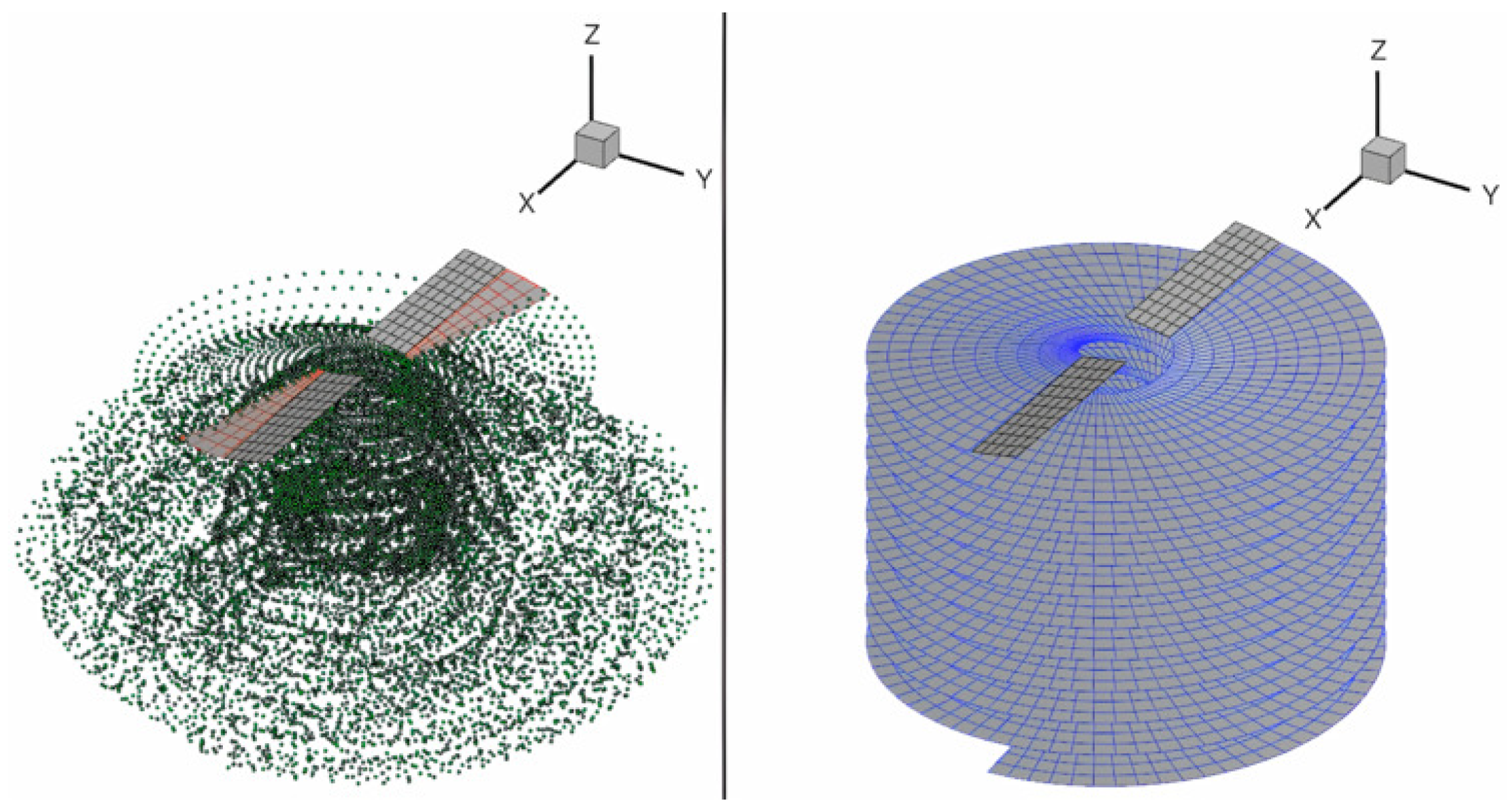
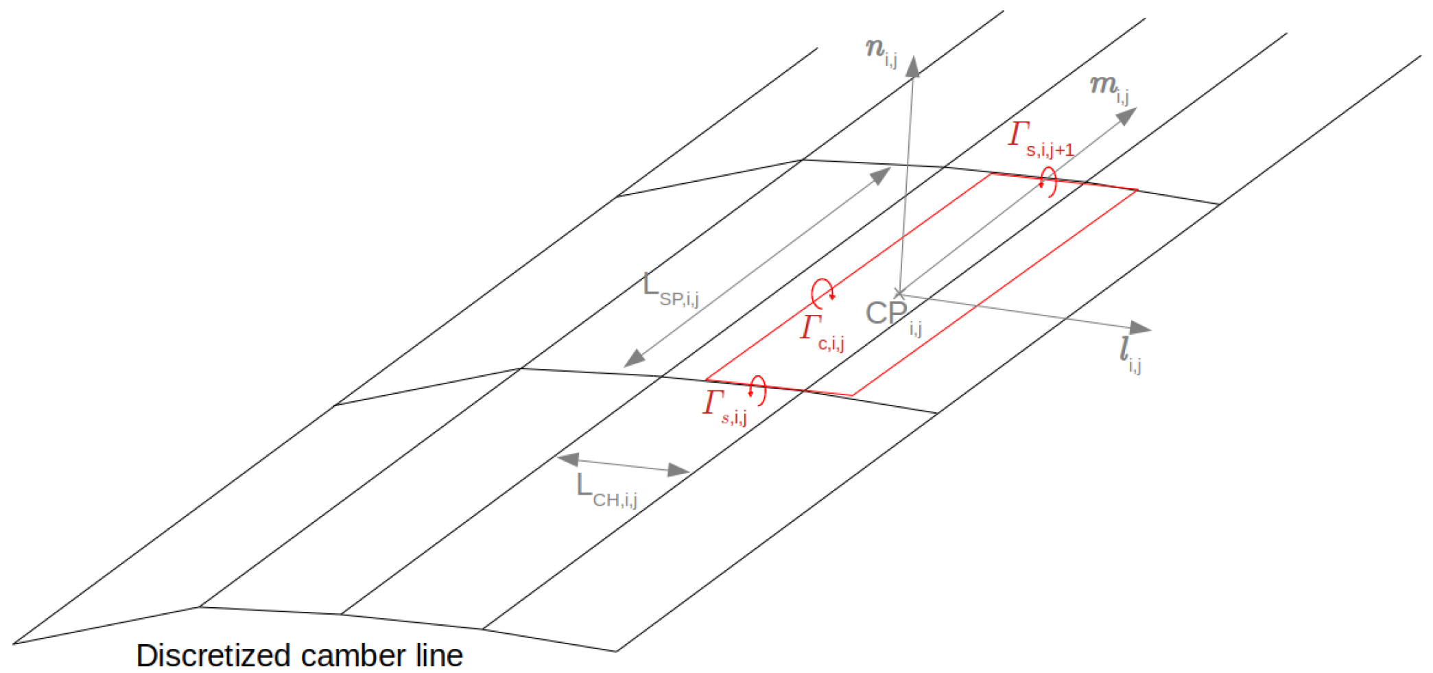
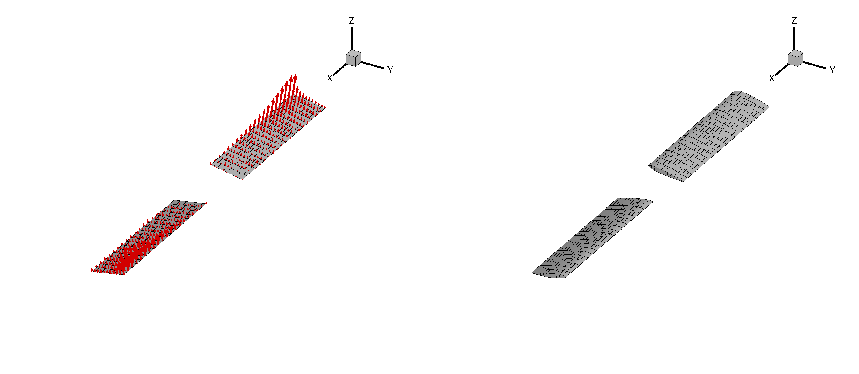

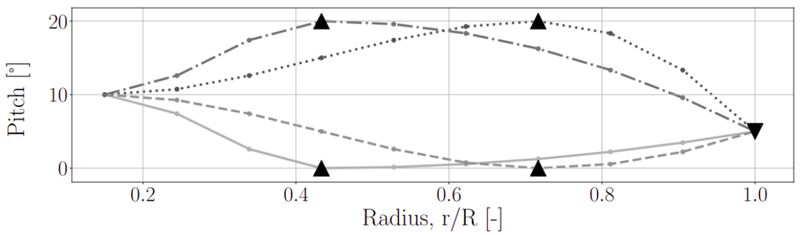

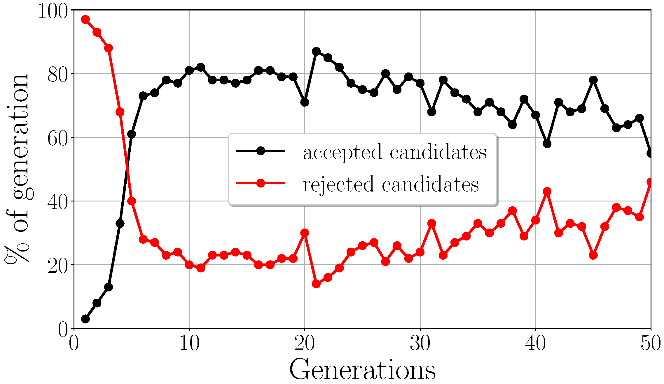
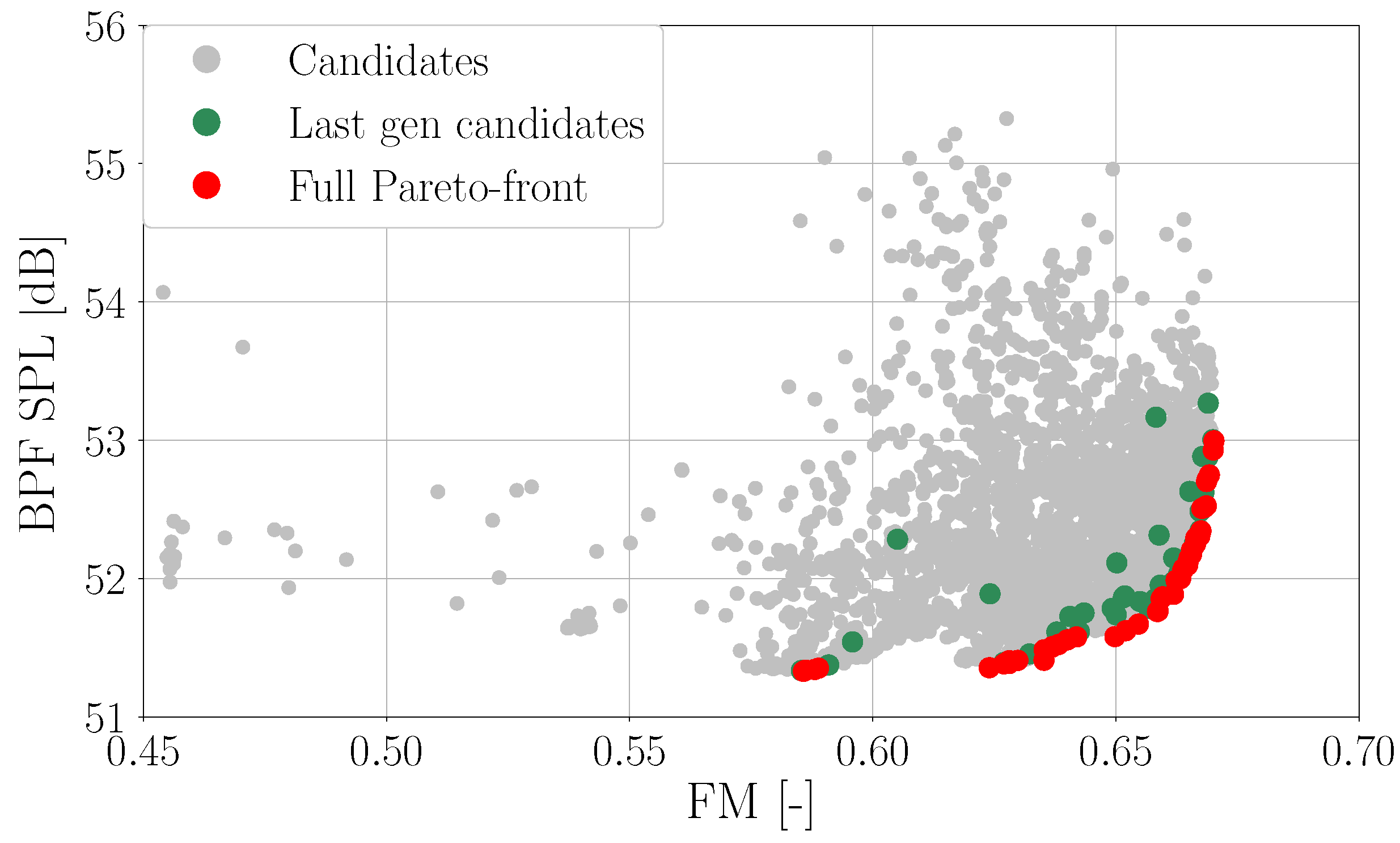
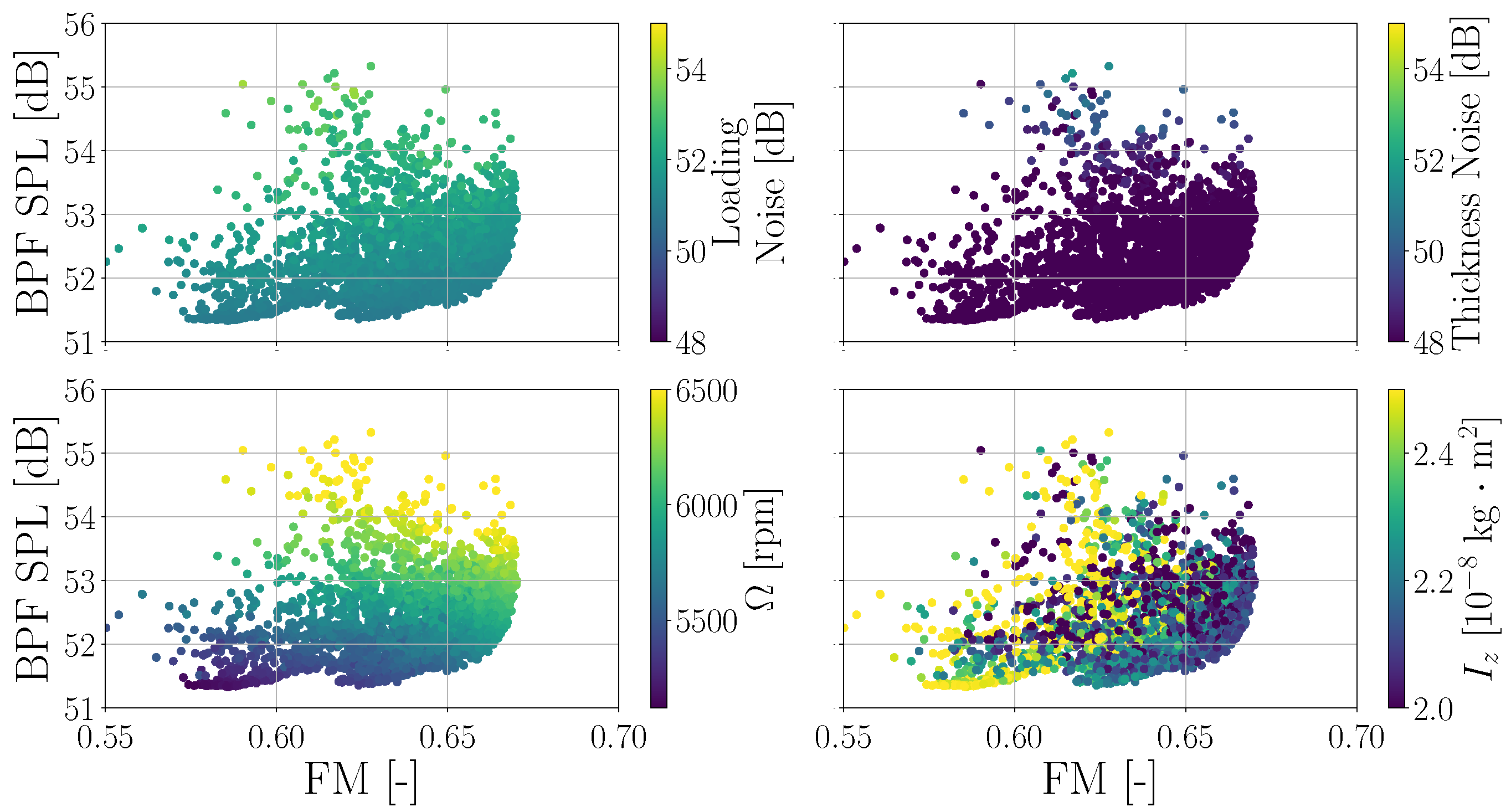
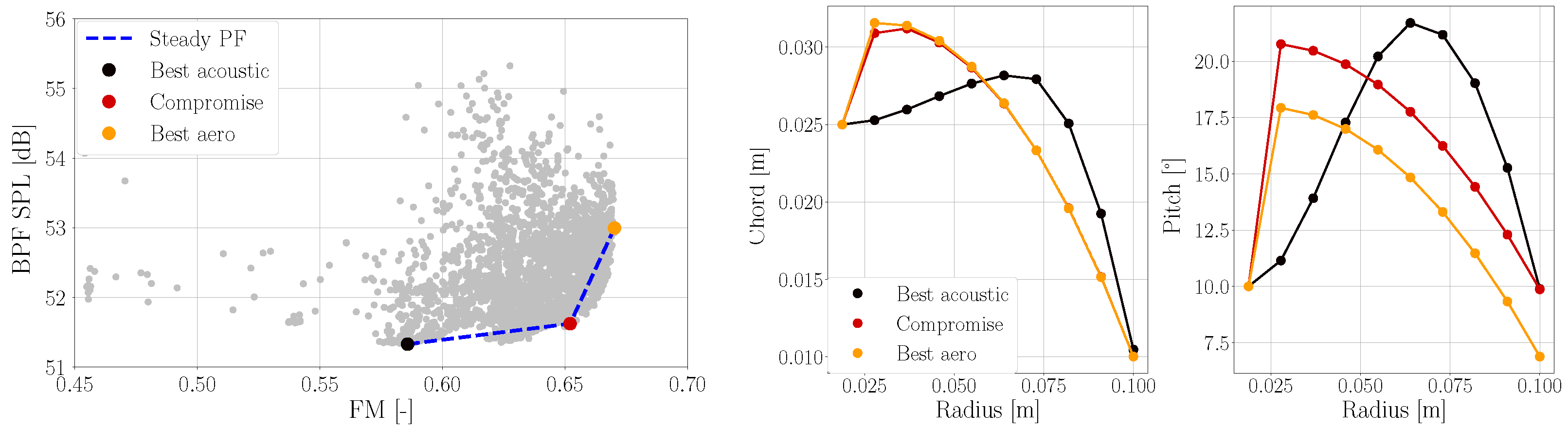
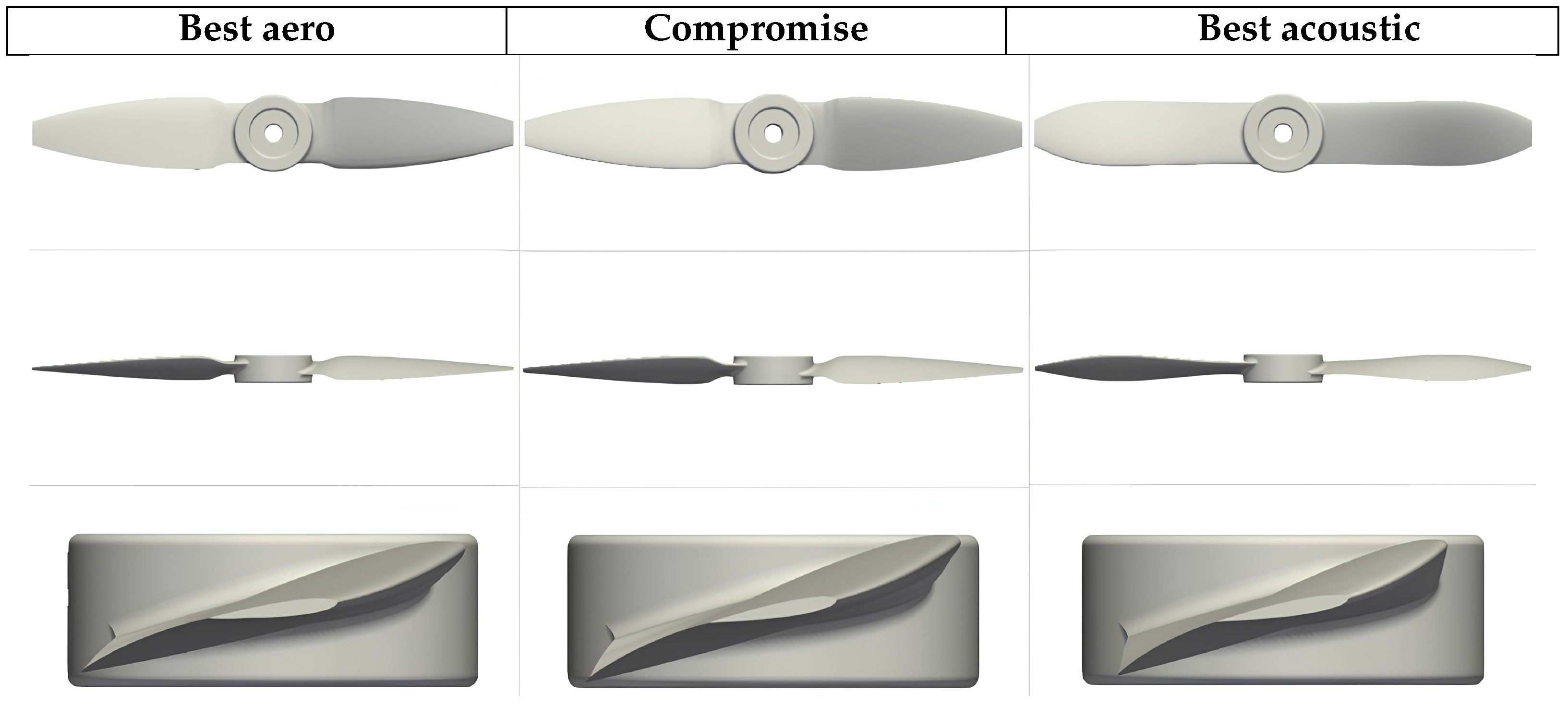
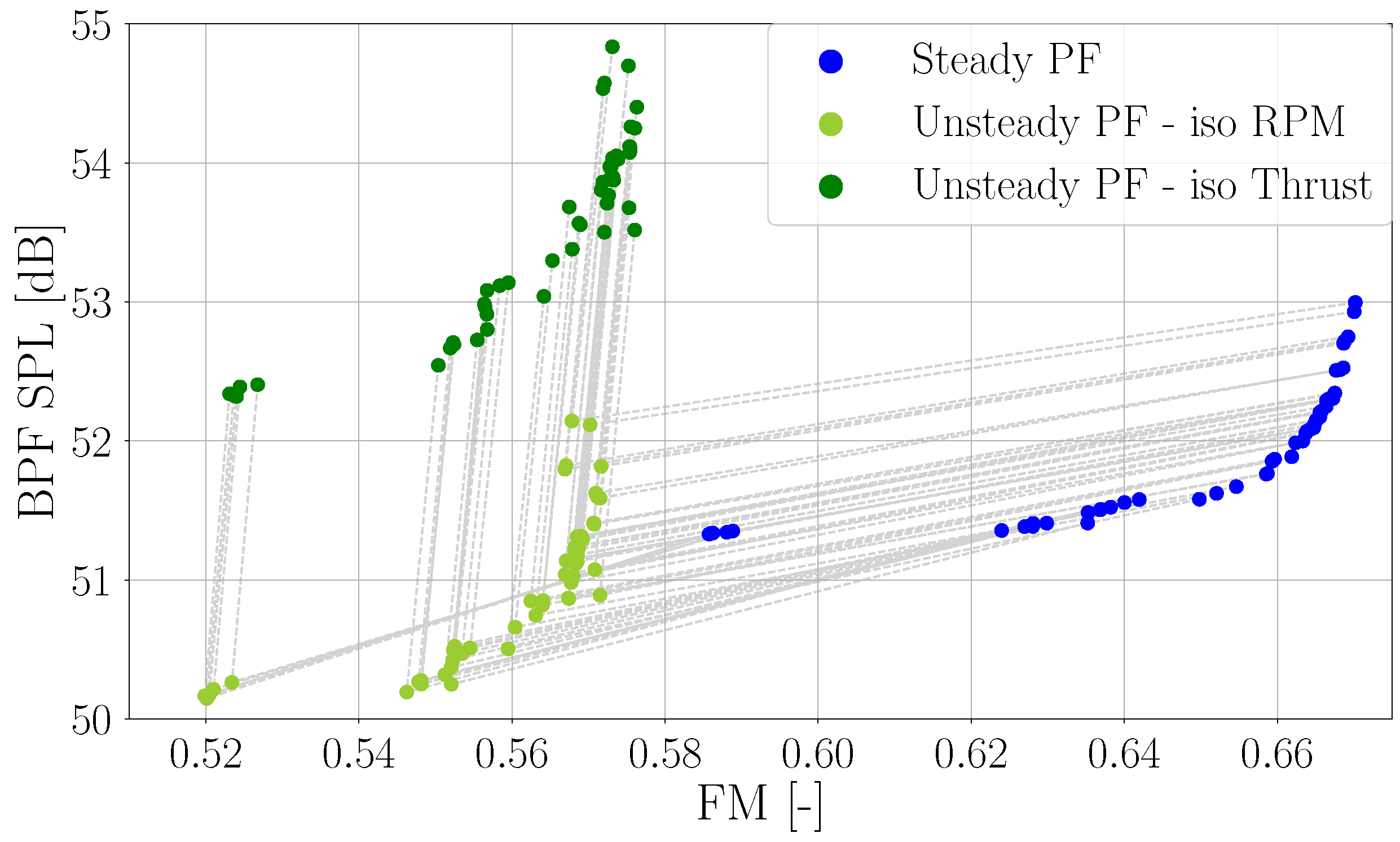
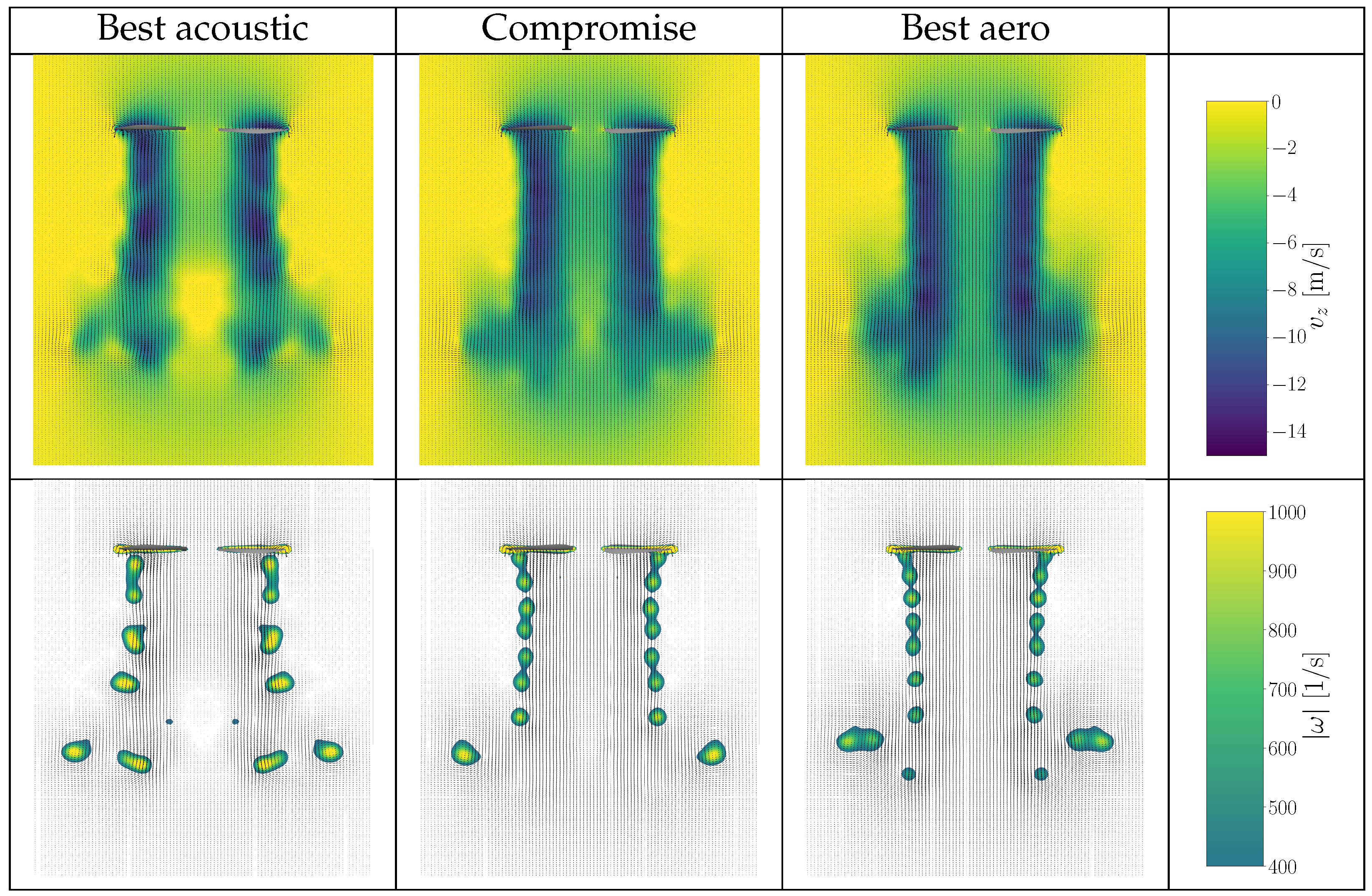
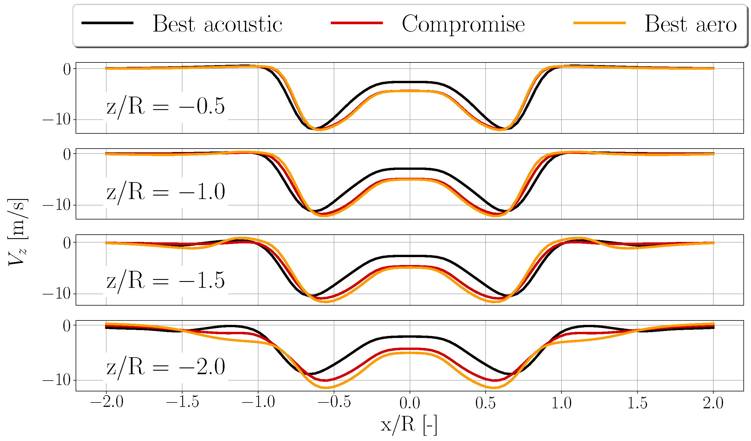

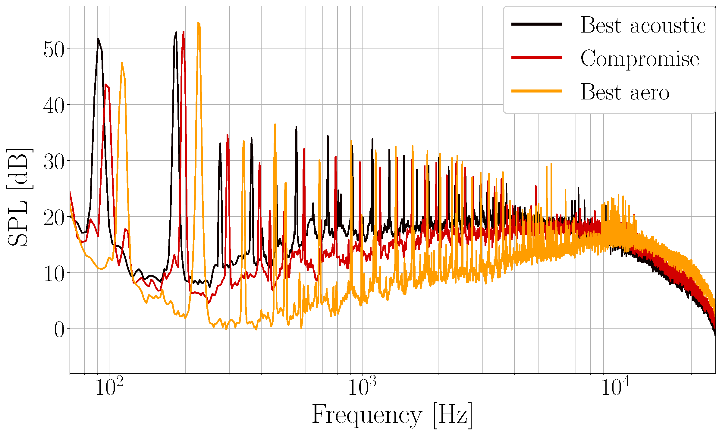
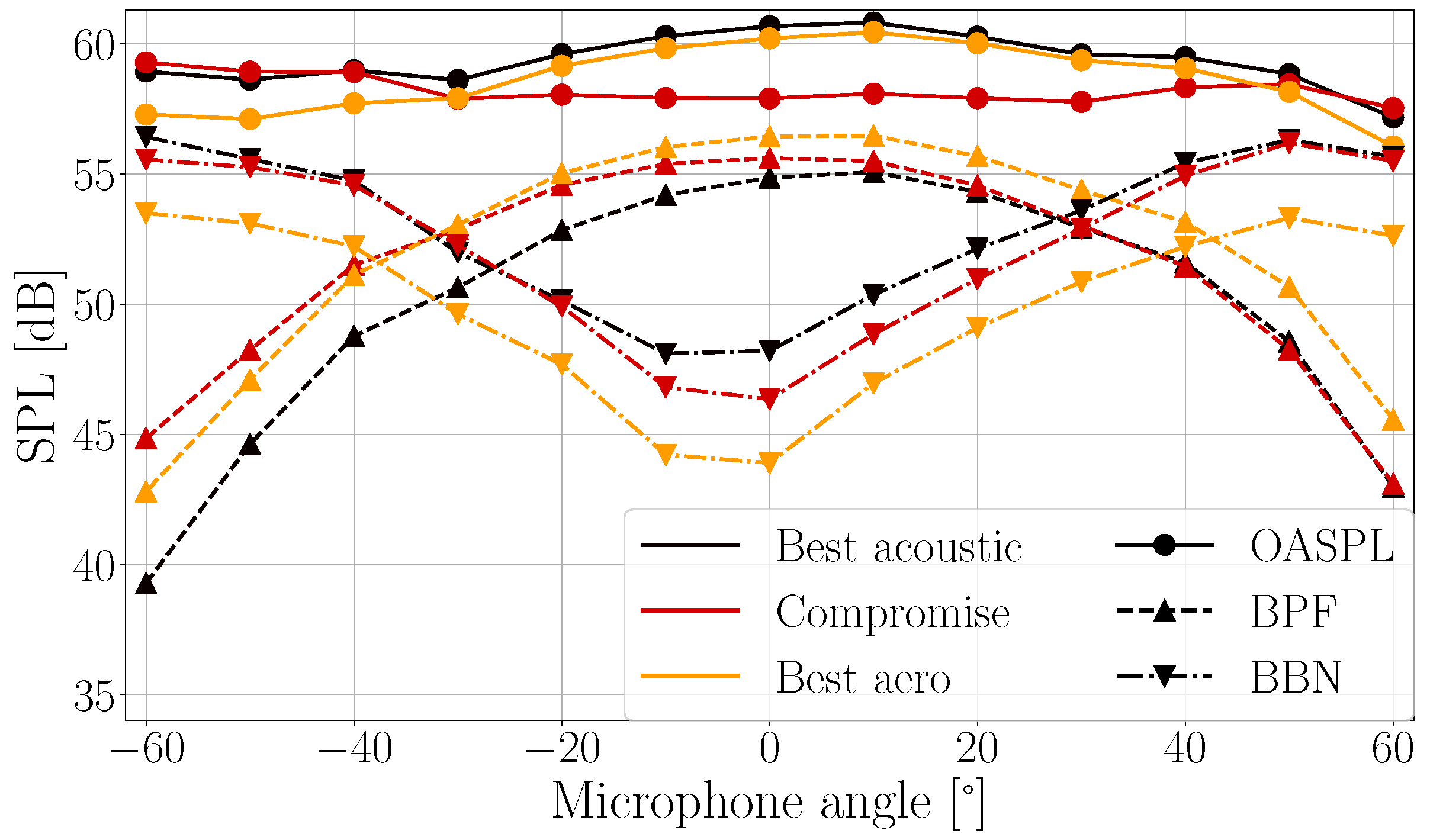
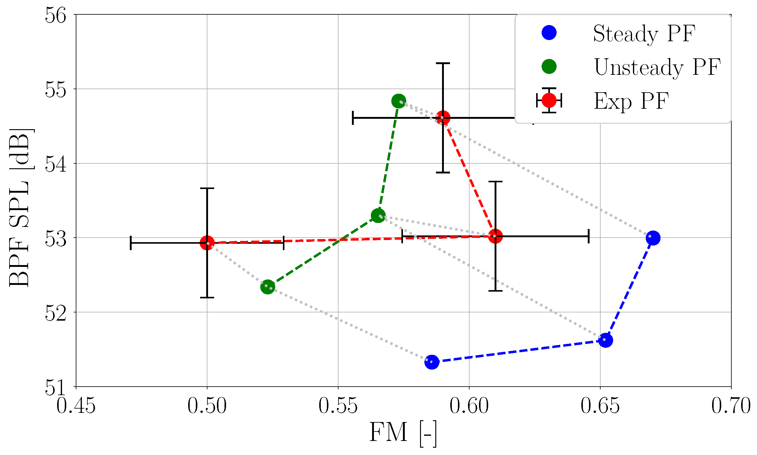
Disclaimer/Publisher’s Note: The statements, opinions and data contained in all publications are solely those of the individual author(s) and contributor(s) and not of MDPI and/or the editor(s). MDPI and/or the editor(s) disclaim responsibility for any injury to people or property resulting from any ideas, methods, instructions or products referred to in the content. |
© 2024 by the authors. Licensee MDPI, Basel, Switzerland. This article is an open access article distributed under the terms and conditions of the Creative Commons Attribution (CC BY) license (https://creativecommons.org/licenses/by/4.0/).