Numerical Simulation of Swept-Wing Laminar–Turbulent Flow in the Presence of Two-Dimensional Surface Reliefs

Abstract

Stochastization of boundary-layer flow has a dramatic effect on the aerodynamic characteristics of wings, nacelles, and other objects frequently encountered in practice, resulting in higher skin-friction drag and worse aerodynamic quality. A swept-wing boundary layer encountering a transition to turbulence in the presence of two-dimensional surface reliefs is considered. The relief has the form of strips of a rectangular cross-section oriented parallel to the leading edge and located at different distances from it. The computations are performed for the angle of attack of −5° and an incoming flow velocity of 30 m/s using the ANSYS Fluent 18.0 software together with the author’s LOTRAN 3 package for predicting the laminar–turbulent transition on the basis of the $e^N$-method. New data on distributions of N factors of swept-wing cross-flow instability affected by the surface relief are presented. The data are of practical importance for engineering modeling of the transition. Also, the effectiveness of using the reliefs as a passive method of weakening the cross-flow instability up to 30% to delay the flow stochastization is shown.

1. Introduction

In cruise flight, boundary layers on surfaces of modem subsonic aircrafts are predominantly turbulent. The accompanying high aerodynamic drag requires searching for new drag reduction techniques by developing different methods of controlling the flow structure in the boundary layers. However, a variety of existing methods of such control, including all kinds of vibrators, actuators, micro-electro-mechanical systems, riblets, large vortex break-up devices, etc., are mainly limited to two-dimensional turbulent boundary layers (see, e.g., [1,2,3,4]).

In three-dimensional flows of the boundary-layer type, as with a swept wing, the main factors affecting the natural flow stochastization are boundary-layer instabilities leading to the development of Tollmien–Schlichting waves (TSWs) and cross-flow vortices (CFVs). The transition to turbulence caused by the development of TSWs occurs mainly in two-dimensional boundary layers. The waves are suppressed quite well by modifying the stream-wise pressure gradient (Natural Laminar Flow (NLF) technique). In three-dimensional boundary layers characterized by strong cross-flow (swept wings, bodies of revolution at high angles of attack, flow near a rotating disk, etc.), the stationary CFVs become the dominant type of instability responsible for laminar–turbulent transition (LTT) onset (see, e.g., [5]) as they appear at relatively low Reynolds numbers [6]. In the transition region, such boundary-layer flow is dominated by turbulent wedges appearing randomly; this, in engineering applications, is described using the intermittency concept. It is based on the assumption that turbulence appears point-wise randomly, when the growing CFVs deflect the base laminar-flow velocity by a threshold value. The evolution of corresponding intermittency coefficient is based on a statistical description of the wedge development [7].

In contrast to the TSWs, the development of CFVs cannot be suppressed with the NLF technique, as the required negative stream-wise pressure gradient intensifies the CFVs. The suppression of CFVs within the natural laminarization approach necessitates thinning the wing and/or reducing its sweep angle, which leads to serious technological difficulties and usually requires a reduction in flight Mach number. While the latter limitation may be acceptable for short-haul aircrafts, it is unacceptable for long-distance flights.

One of the possible solutions to delay the appearance of random turbulent wedges, followed by the stochastization of the swept-wing boundary layer, is hybrid (both active and passive) laminarization with the application of local suction near the leading edge for the suppression of CFVs at the stage of their initial amplification together with the optimization of the airfoil shape downstream. However, a proper organization of suction of this kind is a complex technical and technological challenge, as it significantly affects the internal structure of the wing and increases its weight and cost. To date, similar disadvantages associated with the complication of wing design have not been overcome using another method of laminarization with the plasma actuators placed in the swept-wing boundary layer [8]. Generally, these examples indicate that from the point of view of technical and technological readiness, passive methods of controlling the flow stochastization in a swept-wing boundary layer, which do not require energy input and intervention in the wing structure, are more preferable. These methods include the application of various isolated specially shaped obstacles and/or structured relief on the wing surface.

The technique of targeted changes of boundary-layer characteristics by means of structured surfaces is not new, in principle. For example, the well-known riblets (longitudinal grooves used to reduce turbulent skin friction) [9], various two-dimensional humps and steps [10,11], and distributed roughness elements located near the attachment line, where CFVs start to grow, Refs [12,13] are examples of such structured reliefs.

In some experiments [14,15], a passive method of stochastization delay in swept-wing boundary layers was proposed. It utilizes a structured surface relief consisting of strips with a rectangular cross-section, which are placed parallel to the leading edge or at an angle greater than the sweep angle. The idea of the proposed method is to modify the cross-flow near the strips in such a way as to weaken the downstream growth of linearly developing or weakly nonlinear CFVs and, thus, to delay the appearance of turbulent wedges. Recently, some experimental studies [16,17] were devoted to clarifying the role of the relatively high forward-facing steps in enhancing the amplitude of forced CFVs in the vicinity of the step that accelerates the transition to turbulence. They also contain an extended discussion on previous studies related to the interaction of the CFVs and different two-dimensional gaps and obstacles. It seems that the main difference between these studies and the experiments of [14,15] is in the shape, height, and location of obstacles. In the latter experiments, the upstream relief element was mainly located close to the line of loss of linear boundary-layer stability, whereas in the studies of [16,17] the forced (high-amplitude) vortices experienced clear nonlinear behavior at the step. Meanwhile, at the lowest step height, a transition delay was also observed [16,17]. However, as far as we know, no attempt was undertaken to numerically verify the experiments of [14,15], when the linear development of CFVs was assumed.

It should be noted that state-of-the-art DNS studies related to the transition in swept-wing boundary layers (see, e.g., [18,19]) are too expensive to be used in real-life engineering practice. Currently, for many types of transition controls in aerodynamic applications, one of the most computationally efficient methods to predict the shift of transition to turbulence is tracing the change in the growth of disturbances (see, e.g., [16,18,20]). Particularly, it is well-suited for a so-called ’natural’ or unforced transition, when the disturbances have a long stage of linear development. By definition, the N factors are the values on the envelope of growth-rate curves for linear instability waves of different frequencies. It is usually assumed that as soon as at least one of the waves reaches a critical value, it triggers a transition [21,22]. This approach called the $e^N$- or $exp\left(N\right)$-method has already been proven in numerous studies to work, giving quite good estimations for the transition onset if the critical value is chosen correctly. Available calibrations of the method for different free stream and boundary conditions operate quite well in two-dimensional flows with only one type of instability [23,24]. In three-dimensional flows, when both the Tollminen–Schlichting and the cross-flow instabilities compete, the application of the method is more involved because it is necessary to trace two different N factors. Nevertheless, when the regions of instabilities are spatially separated, the $e^N$ method provides quite good estimations of the transition onset in a wide range of boundary and initial conditions [25,26]. When the instabilities interplay, as in some regions of the boundary layer of an inclined prolate spheroid, neither the $e^N$-method nor other popular empirical approaches can predict the turbulence onset reliably in these regions without additional tinkering [25,26].

In the present study, the $e^N$-method accompanied by a numerical computation of laminar–turbulent flow at Mach number $M\ll 1$ at a swept wing with the surface relief elements is carried out. The main goals of the study are to numerically verify the experimental technique proposed in [14,15] to attenuate the growth of linear CFVs to identify the mechanism of stochastization delay, and to obtain some qualitative hints for the most appropriate geometry and location of surface relief.

2. Problem Formulation and Solution Procedure

The computational domain (Figure 1) is a box with a swept wing placed in it. The domain corresponds to the geometry of the test section of the T–324 wind tunnel of ITAM SB RAS, Novosibirsk, Russia, in which the corresponding experimental studies of the cross-flow instability were carried out [14,15]. The size of the computation box is $5.245\times 1\times 1$ m³ in $x,y,z$ coordinates, respectively. The wing based on a NACA 67 1-215 profile has a sweep angle of ${45}^{°}$; its chord length $C=0.7$ m. It is located at an angle of attack $\alpha =-5^{°}$ to provide the flow stochastization dominated by the cross-flow instability at the upper surface. Note that the swept-wing shape, its position, and sweep angle closely resemble the experimental setup used in the accompanying experiments (see [14,15] for details).

A ‘global’ Cartesian coordinate system was used such that the x-axis is directed parallel to the side walls of the virtual test section, and y and z are vertical and horizontal transversal axes, respectively. The origin of the coordinate system is located at the point on the leading edge of the wing at the zero angle of attack nearest to the inflow boundary. Note that when the angle of attack is $\alpha =-5^{°}$, the origin of the coordinate system is fixed, but the position of the wing relative to the axis of rotation marked in Figure 2 by a dashed line changes. To represent data on the flow stochastization, the ‘wing-oriented’ Cartesian coordinate system was used, such that $x^{\prime }$ and $z^{\prime }$ axes coincide with the chord and wingspan directions, respectively, with the origin at the leading edge and $y^{\prime }=y$. In the third ‘local’ Cartesian coordinate system, $x^{*}$ is directed along a selected inviscid streamline, $y^{*}$ is the wall-normal direction, and $z^{*}$ is the local cross-flow direction. This system is used to show the effect of the relief on the local cross-flow velocity profiles.

The computations of a subsonic swept-wing boundary layer with surface relief elements were carried out using the approach proposed in [27]. The approach includes two main stages: (1) obtaining the characteristics of the main flow with the required laminar part using the ANSYS Fluent 18.0 software, and (2) performing a local stability analysis of the velocity profiles of the laminar boundary layer using the LOTRAN 3 software package to obtain the distributions of N factors of growing vortical disturbances.

At the present time, the $e^N$ method is not implemented in general-purpose gas-dynamic software such as ANSYS Fluent, OpenFOAM, etc. Instead, its different implementations are used as separate plug-ins (see, e.g., [25]). The LOTRAN 3 software developed in ITAM SB RAS is an advanced N-factor method for the automatic prediction of LTT onset in compressible and incompressible three-dimensional boundary layers. The implementation of the $e^N$ method used in the present study has already been validated for a plate, spheroid, and nacelle at different angles of attack in [27], where a comparison with results of other computations is presented.

Within the LOTRAN 3 software, the evolution of small perturbations in a boundary layer is described on the basis of full heat and mass transfer equations of a compressible fluid (also known as Navier–Stokes equations) linearized with respect to the laminar flow. The LOTRAN 3 operation is organized into the stages of main flow data assimilation, the generation of a set of inviscid flow streamlines (processed at the boundary-layer edge and projected to the wing surface), stability analysis of wall-normal velocity profiles along the streamlines, and the determination of distribution of N factors (the envelope) over a flow-exposed surface. The entire sequence of the operations is fully automatic. The estimation of transition position in a three-dimensional boundary layer is reduced to compute the transition onsets in two-dimensional wall-normal cuts along selected inviscid streamlines. In each cut, a series of wall-normal boundary-layer velocity profiles is analyzed. The analysis is based on the solution of eigenvalue problems formulated for ordinary differential equations of propagation of three-dimensional disturbances based on linearized heat and mass transfer equations for a viscous compressible fluid (see [27] for a detailed description). The position of LTT onset is found from the estimation of disturbance growth coded in the distribution of N factors with a user-defined or predicted critical N factor for the transition to turbulence. Then, the position of LTT onset and an estimated length of flow randomization due to the development of turbulent wedges (see, e.g., [28]) are used to characterize statistical intermittency evolution. The obtained intermittency distribution is transferred back to the general-purpose gas-dynamic package (ANSYS Fluent 18.0 in the present case). This is performed with the help of a user-defined function that modifies the turbulent viscosity of a selected turbulence model accordingly.

In the present case, the main flow required for the analysis was precomputed by the ANSYS Fluent 18.0 software. The main flow was obtained based on the solution of three-dimensional Reynolds-averaged Navier–Stokes equations, with the turbulence generation suppressed up to 0.75 wing chord length by an initially specified intermittency distribution to obtain an extended region of laminar flow for further analysis. In solving this, we used a density-based solver, an implicit scheme of the second order of accuracy in space with the Roe-FDS method of convective flow splitting, and the $k-\omega$ SST turbulence model. The thermal conductivity of the gas was given by a formula from the kinetic theory, the viscosity was given by Sutherland’s law, and the heat capacity was set to be constant. The flow velocity and atmospheric pressure were set at the inlet and outlet boundaries, respectively; at the lateral boundaries, corresponding to the walls of the virtual wind tunnel and on the surface of the wing, the no-slip conditions and adiabatic temperature were set. The resulting main flow data were converted to the internal LOTRAN 3 representation with the help of the ANSYS Fluent 18.0 user-defined function. The laminar flow was processed by the LOTRAN 3 package along selected inviscid streamlines. This allows us to estimate a distribution of the N factors over the surface, from which a line of the flow stochastization initiation (the position of LTT onset) is estimated for a selected value of the critical N factor.

The strips of the rectangular cross-section covering the entire wing span (‘two-dimensional’ strips) have a height of 0.28 mm, which does not exceed one-third of the local boundary-layer displacement thickness, and a length of 3.0 mm. They were placed on the upper (windward) surface of the wing parallel to the leading edge at different distances: single-strip reliefs at 10% (Case 1) or 20% (Case 2) of the wing chord (see Figure 2); and double-strip reliefs composed of two strips at 10% and 20% (Case 3) of the wing chord.

The computational domain was covered by a block regular grid with refinement to the wing surface and to the leading edge (see Figure 1). With respect to the smooth surface with 100 partitions along the x-coordinate, the number of cells was doubled (200 partitions) and the mesh refinement was also applied to the reliefs. The cell skewness and orthogonal quality of mesh at the wing surface are more than 0.7, the aspect ratio is 0.05, and $y^{+}<1$ in the turbulent part of the flow. Also, in designing the computational domain, a separate zone with its own ID for the relief region was allocated to be able to build a more detailed computational grid in it. To correctly compare the main flow and its stability over the smooth and relief surfaces, a similar, more-detailed computational grid was constructed for the smooth wing as well. Thus, the total number of cells of the computational grid amounted to 11 million. The convergence was analyzed as follows: when the computational grid was reduced by a factor of 1.5 in all directions, the laminar flow velocity and N factors changed by less than 1%.

3. Results

To investigate the effect of structured relief on the development of CFV instability, we consider the case of incoming flow velocity $Q=30$ m/s directed parallel to the x-axis. For the correct comparison of N-factor distributions, they were computed along similar directions in the cases with and without the reliefs (see Figure 3a). As seen, the streamlines under consideration computed with the LOTRAN 3 LTT package along the smooth surface (solid lines) and along the surface with the single-strip relief (Case 1) located at 10% of the wing chord (dashed lines) are almost identical.

The required experimental data on the position of LTT onset for the smooth surface were obtained by analyzing thermograms to detect the difference between the cooling rates of the slightly heated surface in the laminar and turbulent regions [29]. The obtained and statistically justified positions of LTT onset were superimposed on the computed N-factor distributions to determine the values of the critical N factors along the streamlines. As the available experimental data were analyzed and averaged in the cross-flow direction only near the central part of the wing (streamlines 4, 5,6 in Figure 3a) [29], the computed data were only averaged for the fourth, fifth, and sixth streamlines. The experiments showed that at $Q=30$ m/s in the boundary layer, without the relief, the transition onset is characterized by the averaged critical value $N_{\mathrm{crit}}\approx 6$.

Figure 3b shows that the application of single-strip relief (Case 1) leads to a shift of the N-factor envelopes for stationary CFVs (dashed curves) downstream and, consequently, results in delayed flow stochastization. The distributed effect of relief is shown by comparing the contours of the constant N factor in Figure 3c. In the case of the smooth and relief wings, the position of LTT onset corresponding to $N_{\mathrm{crit}}=6$ is shown by the white and blue contours marked by ‘6’, respectively. As seen, in the presence of the strip, the contour moves significantly downstream (7–12% of chord length C).

The effect of the presence of the single strip relief at 20% of the chord length (Case 2) and a combination of two single strip reliefs at 10% and 20% of the chord length (Case 3) is shown in Figure 4. These reliefs also attenuate the linear growth of CFVs, so that the critical value $N_{\mathrm{crit}}=6$ is not achieved at all in the stream-wise region under consideration. Note that for Case 2, the attenuation of CFV growth is higher compared to the single-strip relief at 10% of chord (Case 1), and even higher for the combination of these reliefs (Case 3).

It should also be noted that experiments [14,15] show that the rectangular-shaped reliefs shift the flow stochastization by about 15% downstream. Thus, the numerical and experimental data are in qualitative agreement.

4. Discussion

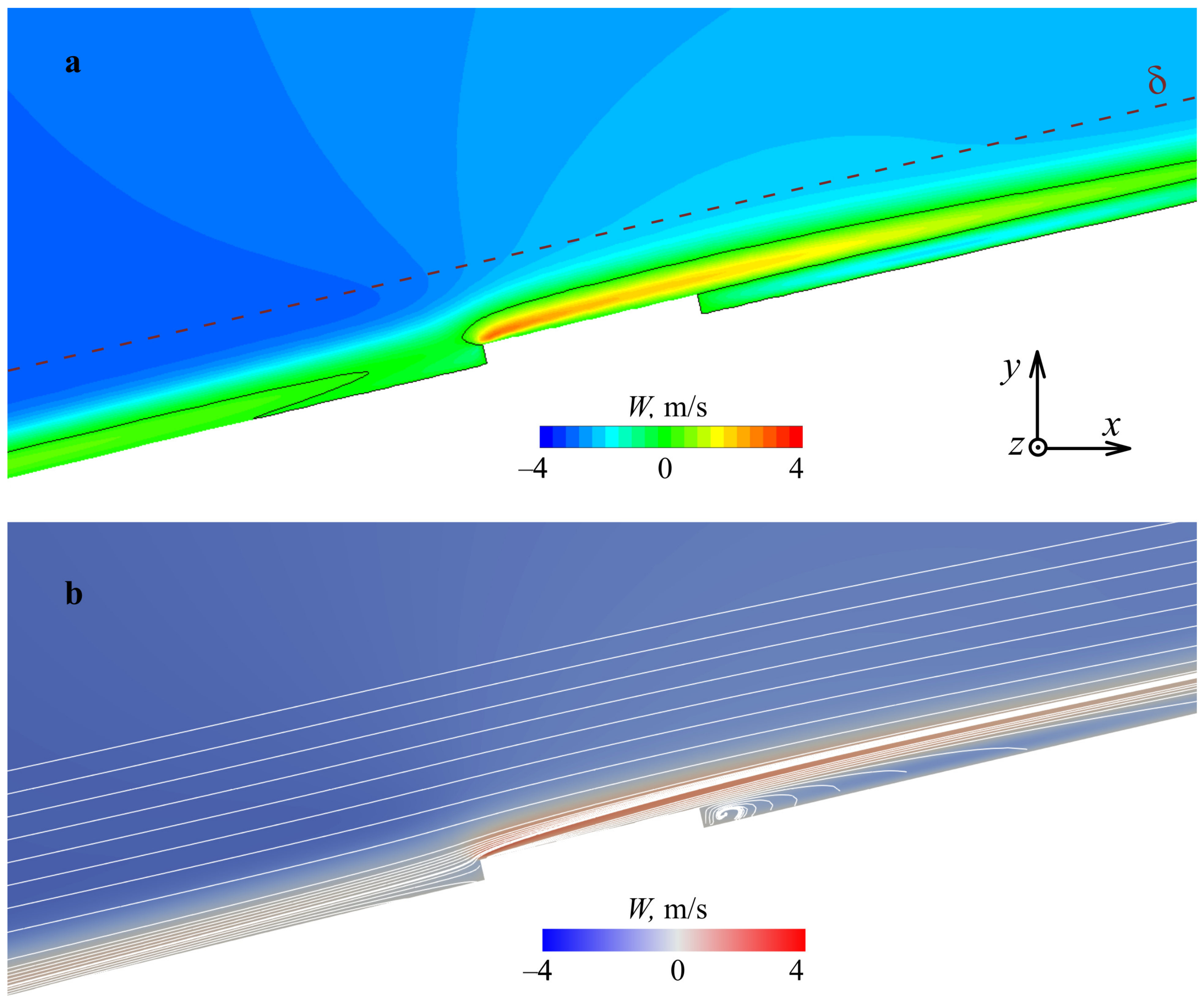
To identify a mechanism of flow control, the corresponding changes in the main flow were analyzed. Results of the computations show that the presence of a single- or double-strip relief leads to the following changes: zones upstream, above, and downstream of the rectangular relief element appear, in which the z-component of velocity is significantly modified (Figure 5a) and vortices near the vertical walls of the relief with axes directed along the strips appear (Figure 5b). The presence of the vortices near the vertical walls of the relief indicates the appearance of local separation zones that are in line with previous studies where similar geometries were considered (see, e.g., [10]).

In Figure 6, profiles of cross-flow velocity $W^{*}$ (in the ‘local’ coordinate system) at several downstream locations along streamline 5 of Figure 3 for the smooth and relief surfaces are shown. The locations correspond to the positions downstream from the relief. As seen, the relief has a significant effect on the local cross-flow velocity at downstream distances exceeding its height (0.28 mm) by several hundred times. First, the value of the cross-flow is reduced. Second, its maximum shifts further away from the wall, as clearly seen in Figure 6b. While the reduced cross-flow naturally indicates smaller growth rates of CFVs; this leads to changes in N-factor envelopes, as shown in Figure 4, and the effect of the shift is a bit more subtle. This results in a change in the ‘effective’ velocity profile, which is a projection of the stream-wise $U^{*}$ and the cross-flow $W^{*}$ velocities to the direction of the wave vector of stationary cross-flow vortex (see, e.g., [30,31] for details). Naturally, the change in the effective profile also contributes to the change in the local stability characteristics of the flow. Note also that the distance of influence is much longer than the typical length of a laminar two-dimensional separation bubble downstream a backward-facing step which deepens into the boundary layer (see, e.g., [32]). This suggests that quasi-two-dimensional considerations (e.g., the presence of laminar separation downstream from the relief) cannot completely explain the flow relaxation in the case under consideration. Indeed, despite the fact that the cross-flow in the boundary layer is typically less than several percentages of the free stream velocity, it is the main factor triggering the linear instability under consideration. Hence, apparent, very small residual changes of the cross-flow can lead to a substantial change in the disturbance growth. This can explain why the second relief element is effective in Case 3. The first strip reduces the growth of the vortex in that does not allow it to reach a nonlinear stage to reach the position of the second strip; then, the second strip further ’disequilibrates’ the boundary layer to prevent vortex growth. Note that the second strip alone (Case 2) is more effective than the first one (Case 1). This means, naturally, that there is an optimal strip position and relative height that one can try to find. This, however, was not a goal of the present study.

In general, as seen from Figure 5 and Figure 6, the boundary layer is in a state of relaxation in response to the undisturbed flow for a considerable distance downstream from the strip, which is accompanied by the presence of a significantly weakened and modified cross-flow velocity necessary for the development of linear CFVs.

5. Conclusions

Comparative computations of laminar–turbulent flow at a swept wing with a smooth surface and relief surfaces, in the form of strips of a rectangular cross-section directed parallel to the leading edge of the wing, were carried out. The computations of base laminar flow in the virtual wind-tunnel test section to mimic conditions of experiments [14,15] were carried out with ANSYS Fluent 18.0 software. The disturbance growth was analyzed with the LOTRAN 3 laminar–turbulent transition prediction package. As in the experiments, the computations were carried out with governing parameters ensuring the dominant mechanism of the flow stochastization through the growth of cross-flow vortices: the velocity of incoming flow $Q=30$ m/s and the wing angle of attack $\alpha =-5^{°}$. The main results of the study are as follows:

• The effectiveness of surface-structured relief in the region of the linear amplification of the cross-flow vortices as a passive method for delaying the flow stochastization was demonstrated; changing the distance of a strip from the leading edge was found to significantly affect the value of the delay; and the sequential installation of several relief elements led to better delay than the separate application of the strips.
• The mechanism of the delay is illustrated: extended zones of modified, weakened cross-flow appear downstream the strips, thus contributing to the reduced instability responsible for the flow stochastization.