Abstract
Compressors are an essential component of aircraft engines. Their design and operation must be extremely reliable as engine safety and performance depend greatly on these elements. Axial compressors exhibit instabilities, such as surge or rotating stall, in a region close to the peak of their performance curves. These fluid dynamic instabilities can cause drops in efficiency, stress on the blades, fatigue, and even failures. Compressors are handled therefore by operating with a safety margin far from the surge line. Moreover, models able to predict onset instabilities and to reproduce them are of great interest. A dynamic system able to describe successfully both surge and rotating stall is the model presented by Moore and Greitzer That model has also been used for developing control laws of the compressor dynamics. The present work aims at developing an artificial neural network (ANN) approach able to predict either the permanence of the system in stable working condition or the onset instabilities from a time sequence of the compressor dynamics. Different solutions were tried to find the most suitable model for identifying the system, as well as the effects of the duration of the time sequence on the accuracy of the predicted compressor working conditions. The network was further tried for sequences with different initial values in order to perform a system analysis that included multiple variations from the initial database. The results show how it is possible to identify with high accuracy both rotating stall and surge with the ANN approach. Moreover, the presence of an underlying fluid dynamic model shares some similarities with physically informed AI procedures.
1. Introduction
With the continuous improvement in the state of the art and technologies, aircraft engines have nowadays reached a very high level of complexity. However, the challenge of finding new solutions that preserve reliability while enhancing performance is compulsory for the next generation of engines complying with the FlightPath 2050 targets [1]. A strategy selected in achieving these goals focuses on active flow control and casing treatment of flow compression systems. In fact, the high-pressure, high-efficiency region of an axial flow compressor lays close to the surge line and to the region where rotating stall may occur, so that optimal operating lines run in a region where the compressor is prone to different kinds of instabilities. For this reason, the surge margin (SM), that is, the distance between the operating point and surge, is monitored in real time by the Digital Engine Control Unit (DECU) to avoid the onset of instabilities. The smaller the surge margin, the higher the performance. This reasoning has motivated wide investigations of compressor instabilities such as classical surge (CS), deep surge (DS), and rotating stall (RS) [2,3,4,5,6]. The detection of the instabilities and their active control are essential tasks in order to ensure safety and engine performance [7,8,9,10,11]. As RS and DS instabilities are nonlinear phenomena, one of the most effective approaches to their control is the model-based predictive control, which in turn requires an underlying reduced order model that predicts the system evolution within a given time interval.
Among the modeling efforts in describing the nonlinear dynamics of rotating stall and surge, the model proposed by Moore and Greitzer (MG) [2,3] was one of the most successful, since it captures the essential features of these instabilities by relating them to some characteristic parameters of the system interacting with the surrounding environment and nearest components. Moreover, the MG model is expressed as a low-order state-space model and this fact makes it suitable for applications to control design. The MG model has been further extended, including other effects, e.g. variable compressor speed, additional control valves, etc., and the availability of such reduced order models also encourages the efforts in developing active control schemes for compression systems [12,13,14,15,16]. Apart from classical PID controllers, a variety of approaches have been used as adaptive control [13], back-stepping [17], bifurcation theory [18], and state-feedback linearization [19]. More recently, other model-based predictive methods have applied artificial neural networks [20], fuzzy logic control [21], and neural network predictive controllers [22,23]. Regarding the devices used for manipulating the flow, although advanced control concepts such as synthetic jets [24] and plasma actuators [25] have been considered, the most widely used actuators over the years remain the Close-Coupled Valve (CCV) [14,19] and the bleed Throttle Control Valve (TCV) [26].
In the present paper, a method based on artificial intelligence (AI) for detecting the onset and type of compressor instability is proposed. The characteristic parameters of an equivalent MG model [27] are extracted by using a deep learning procedure from time sequences of the compressor dynamics recorded by sensors embedded in the system. From the values of such estimated parameters, compressor stability/instability, as well as the near future system evolution, are deduced. In order to test the accuracy and effectiveness of the method, the algorithm is applied to time sequences generated by the analytical MG model itself, without loss of generality. In fact, the MG model can be tailored to a specific compressor by using an experimental fitting of the related map [27,28,29]. To test the proposed procedure, a theoretical/numerical approach is adopted here: we generate a “synthetic” signal by using the MG model and then we analyze the accuracy of the AI-based detection algorithm by comparison with the exact solution.
The paper is organized as follows: the Moore and Greitzer model is presented and some key stable and unstable evolutions are shown; then, the deep learning algorithm is explained and its ability and accuracy in estimating the system working conditions are tested. The algorithm accuracy is then checked against reduced input time sequences. Finally, uncertainty in the initial conditions is introduced and its influence is investigated in combination with the use of reduced length time series in input.
2. Mathematical Model
A sketch of compression system components with related geometrical parameters is shown in Figure 1. The flow enters from atmospheric pressure in the inlet annular duct, proceeds through the compressor block and plenum, where the static pressure is increased to level , and to the outlet duct, from where it exits to atmospheric pressure through the downstream throttle. The plenum and throttle are a quite simple model of simulating the mass storage and mass flow regulation effects of the combustor–turbine–nozzle system in a gas turbine engine [30]. The flow is assumed incompressible, irrotational, and without radial variations, i.e., two-dimensional in the inlet duct. These assumptions hold for low-speed axial compressors with high hub-to-tip ratios. The flow compressibility in the plenum is responsible for mass storage effects.
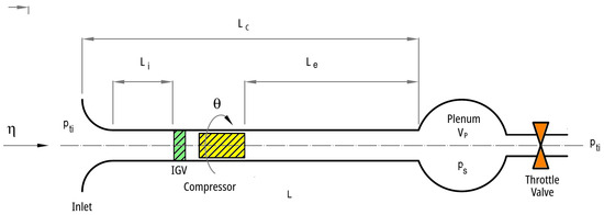
Figure 1.
Sketch of the M-G reduced-order model.
System performances are described by the flow coefficient , i.e., the ratio between the axial velocity component and the compressor speed at the mean radius U and by the total-to-static pressure rise
At steady state, the compressor pressure rise delivered as a function of the annulus averaged flow rate is known as the compressor map . The map is evaluated experimentally and fitted by a polynomial function:
where are coefficients fitting the experimental data and is the annulus averaged flow coefficient
where is the circumferential position, or rotor wheel angle, and is the nondimensional time. Overline is used throughout the paper to defined annulus averaged variables. A similar quadratic relation holds between the pressure drop versus flow rate delivered by the downstream throttle:
where is the pressure drop across the throttle and is the throttle coefficient. Conversely, the relation
is evidence of how the mass flow depends on the throttle setting and the pressure drop. In steady conditions, the pressure rise in the compressor must be equal to the pressure drop across the throttle, and therefore the intersection of the two pressure delivery curves gives the steady state operating point for the compression system, as is indicated in Figure 2a.
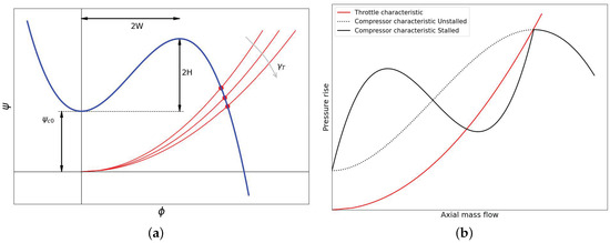
Figure 2.
Compressor–valve characteristics. (a) Map of the unstalled case with different valve opening values (red lines), (b) sketch of the stalled case.
From the continuity equation written for a lumped volume across the compressor and the isentropic relation [3], one derives
by introducing the mass flow coefficient and collecting some parameters that characterize the system setup
the lag in the pressure rise can be derived as
where is the aerodynamic length of the compressor
where is the number of stages, is a time-lag parameter, and is a parameter taking into account for flow inertia on the response to perturbation traveling in the axial direction. It depends on the effective path inside the compressor being longer than its axial length. This consideration is evident modeling the row time-lag ; e.g., a proposed estimation is [2]. The parameter is known as the Greitzer surge parameter defined by
where and are the volume and the speed of sound in the plenum, respectively, and is the flow area.
The flow acceleration rate through the compressor is derived from the axial momentum equation applied from the upstream ambient to the plenum [2]. At the axial station () in front of the compressor/IGV is
where accounts for the fluid inertia in the rotor. An evolution equation for the flow disturbances is now derived to focus on the flow instabilities. The flowfield variables are divided into annulus averaged and circumferential perturbation components
The overline defines annulus averaged quantities, i.e., and indicates a perturbation quantity; i.e., is the perturbation of the flow coefficient. By averaging both members of Equation (11), the axisymmetric part is obtained as
whereas the non-axisymmetric part of (11) is derived by subtracting (13) from (11), that is
Moreover, the incompressibility assumption in the inlet duct region allows us to define a perturbation velocity potential , such as , which satisfies the Laplace equation
inside the inlet duct. The solution for is of the form
where and are amplitude and phase of the n-th circumferential Fourier mode, respectively. The perturbation of the flow coefficient is then
The solution for the flow perturbation is evaluated at the rotor face. Based on this potential flow solution, the perturbations of the downstream static pressure and upstream total pressure are given by [12]
Combining Equations (14) and (15), a relation for non-axisymmetric unsteady behavior in the compressor annulus is derived:
The set of Equations (6), (13) and (19) describe the behavior of an axial flow compression system. A further simplification of the equation set is obtained by applying the Galerkin procedure and then retaining the first term in the Fourier series of the perturbation only.
Finally, assume and introduce the most suited formulation of as a cubic of the form
where are the semi-height, the semi-width, and the shut-off value, respectively, of the curve shown in Figure 2.
The simplest formulation of the MG [2,14] model becomes
where is the squared amplitude of the flow perturbation also identified as the rotating stall amplitude.
The equations presented in (21) account for a variety of phenomena and features of the compression system, such as system volumes, inlet and diffuser shapes, axisymmetric compressor characteristics, throttle characteristics, system hysteresis, compressor geometry, and internal lag processes in the subsystems. Modifications of the MG model to include effects generated by inlet distortion, compressibility inside the compressor, rotational speed variation, and many other improvements have been proposed from other researchers [14,18,31,32,33].
Numerical Simulations Based on the Moore and Greitzer Model
Some typical solutions obtained by integrating the MG model numerically are presented in this section. The main parameters of the model used are shown in Table 1. The four configurations selected, each one representing a possible scenario described by the MG model, are:

Table 1.
Values of Moore and Greitzer parameters.
- (a)
- Stable working point;
- (b)
- Rotating stall;
- (c)
- Classical or deep surge;
- (d)
- Mixed instability.
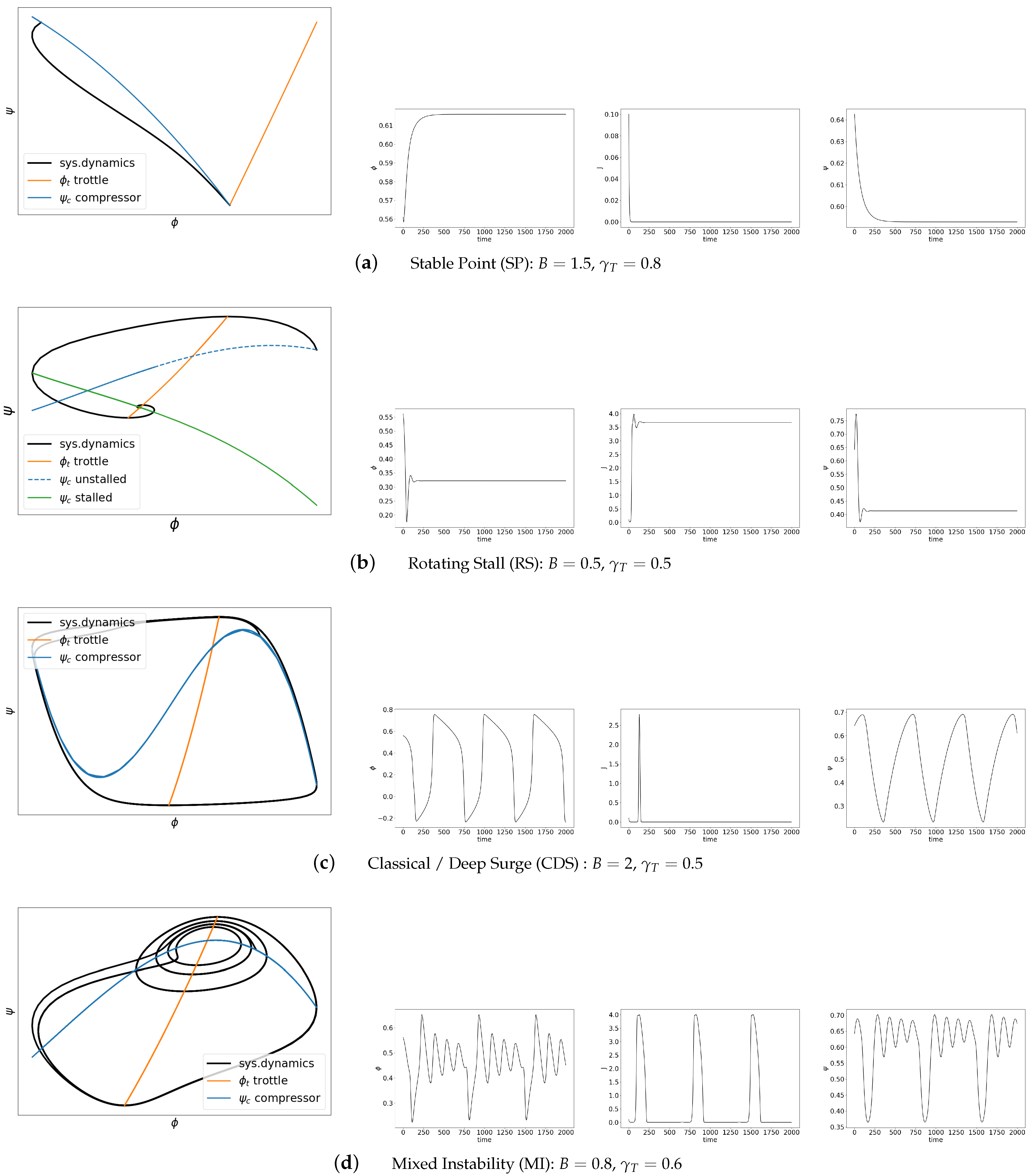
The numerical integration is based on the fourth-order Runge–Kutta method. For all cases, the initial working condition is the same , whereas the different dynamics corresponds to different values for the parameters B e . The trajectories in the compressor map () and the evolutions in time of all the system variables , , and are presented in Figure 3 for completeness. The cases (a), (b), and (c) in Figure 3 are typical scenarios the AI detection algorithm should deal with. Case (d), namely the mixed instability, is the most confusing but also of great interest since it describes the system falling in rotating stall/surge. Actually, the system finally ends up in surge so that, in this case, RS is acting as a precursor of surge. The results are discussed, together with our findings, in the next sections.
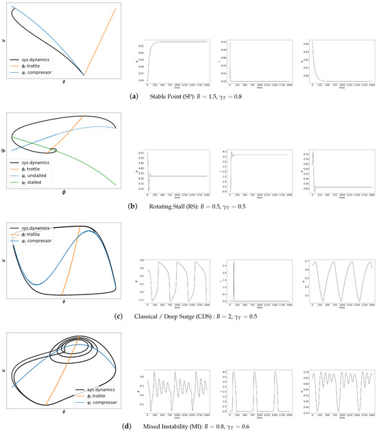
Figure 3.
Four typical dynamics resulting for the same initial conditions and different parameter setup of Moore and Greitzer model. For each case, the plot of and the evolution in time of , and are presented (from left to right).
3. Description of the AI-Based Approach
Artificial intelligence (AI) is an overall definition of a science that contains several fields within it. This work focuses on the use deep learning (DL) approach based on artificial neural networks (ANNs). Briefly, an ANN is formed by an interconnection of nodes, called neurons, which represent the information processing units. They are organized into layers which can be recognized as input, hidden, or output layers. An example of a feed-forward neural network, where the neurons send signals only in one direction, is shown in Figure 4a. The number of input neurons corresponds to the input variables of the system, while the number of output nodes equals the number of outputs associated with each input. In Figure 4b, it is possible to identify three basic elements of the computational model: (i) a set of connected synapses, each one characterized by a weight, which could be either positive or negative; (ii) an adding junction to sum or combine the input signals; (iii) an activation function to introduce non-linearity into the system.
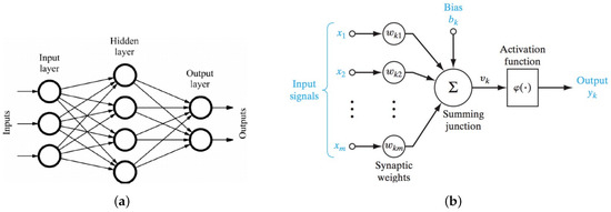
Figure 4.
Sketch of (a) the feed-forward neural network and of (b) the artificial neural network scheme adopted for TensorFlow.
In order to monitor the training of the neural network, a loss function is defined to compare the target and the predicted output, measuring the model performance. The training of a deep neural network consists of two essential phases: forward propagation and backpropagation. In the first one, the input data are given to the model to generate predictions, and the error from the target value is calculated through a suitable loss function. Secondly, to minimize this loss function, the network works backwards from the output, iteratively updating the coefficients of the nodes (weights). Therefore, the backpropagation is a required method used in supervised learning to reach the proper level of model performance.
The main goal of the present work is to estimate the relationship between time series of independent variables, i.e., the input feature, and the parameters B and of the governing equations, namely the targets, that characterize the system dynamics. Therefore, the neural network will be used here to solve a regression problem.
To build and train the neural network, we used TensorFlow, an end-to-end open-source platform for machine learning [34]. It provides an extended system of libraries, tools, and resources that helps to create efficient machine learning models, especially those implementing neural networks [35]. TensorFlow is a platform already extensively used for fault detection and diagnosis [36,37], also recently introduced for axial compressors [38,39,40].
The API we used in the TensorFlow library is Keras, which allows for flexible and modular access to the construction of the model, simplifying experimentation with different configurations and architectures [41,42].
The dataset is partitioned into three smaller ones, namely the training, validation, and test datasets. The validation dataset evaluates the accuracy of the model built on training data, whereas the test set is used to double-check the model. By following best practice guidelines [35], the dataset partitioning in the present study was set as follows: Training = 64%, Validation = 16%, Test = 20%.
ANN Model Definition
The feed-forward neural network is implemented in Python using the Keras functional API [43], which allows models with multiple inputs and outputs. The model architecture is based on fully connected layers; that is, each neuron is connected to every neuron in the previous layer. The target values of B and have been normalized in the range [0–1] by using the MinMaxScaler function of the Scikit-learn library [44].
The input layer, i.e., the first layer of the neural network, receives the data to initialize a Keras tensor. In the present case, each element of the input dataset is a vector
with N = 1000 in our computations. Therefore, each element consists of a time sequence describing the evolution of the independent variable , , at N times steps , starting from the same initial condition
but characterized by the parameters and . The time series of the RS amplitude J is enclosed between square brackets since in the reduced input dataset its evolution has been neglected in the training process. The ANN output is the estimated value , of the parameters B and , respectively. Seven layers have been introduced between the input and output layers. The parameters and functions for each layer are presented in Table 2. A single ANN model is trained for obtaining both outputs. The convergence of the ANN training process is monitored by the MeanAbsoluteError loss function [34], whereas the Adaptive Moment Estimation (Adam) algorithm has been used as the optimizer. The latter combines the advantages of both the AdaGrad (Adaptive Gradient) and RMSprop (Root Mean Squared Propagation) approaches, from which it takes the adaptive learning rate and the moving average of squared error, respectively.
Table 2.
Neural network parameters.
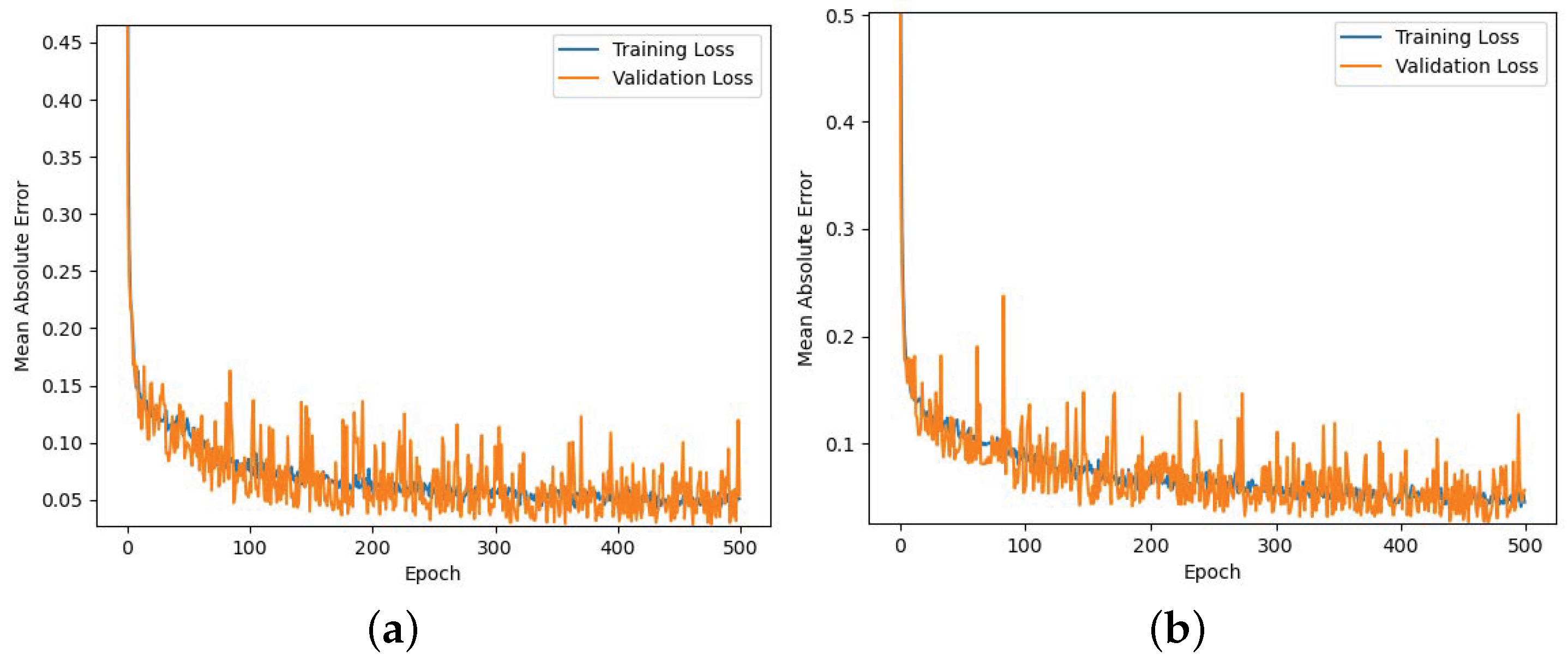
As mentioned, two different models have been trained, one considering the full input dataset and a reduced dataset with only. Results on the convergence of the training process are shown for both datasets in Figure 5. These plots show similar convergence rates, with a small improvement for the full dataset case, since the convergence of the validation step is closer to that of the training step. Nevertheless, we observed that the ANN model trained with the reduced dataset leads to more accurate predictions of the system dynamics. In fact, the time evolution of vanish very rapidly in most cases, except in rotating stall, so that by including the J-time history in the training process, the overall convergence error is reduced without improving the detection of instabilities.
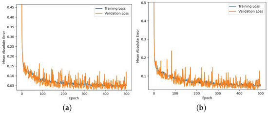
Figure 5.
Loss function residuals of the ANN training using (a) the full set of time series and (b) the reduced set .
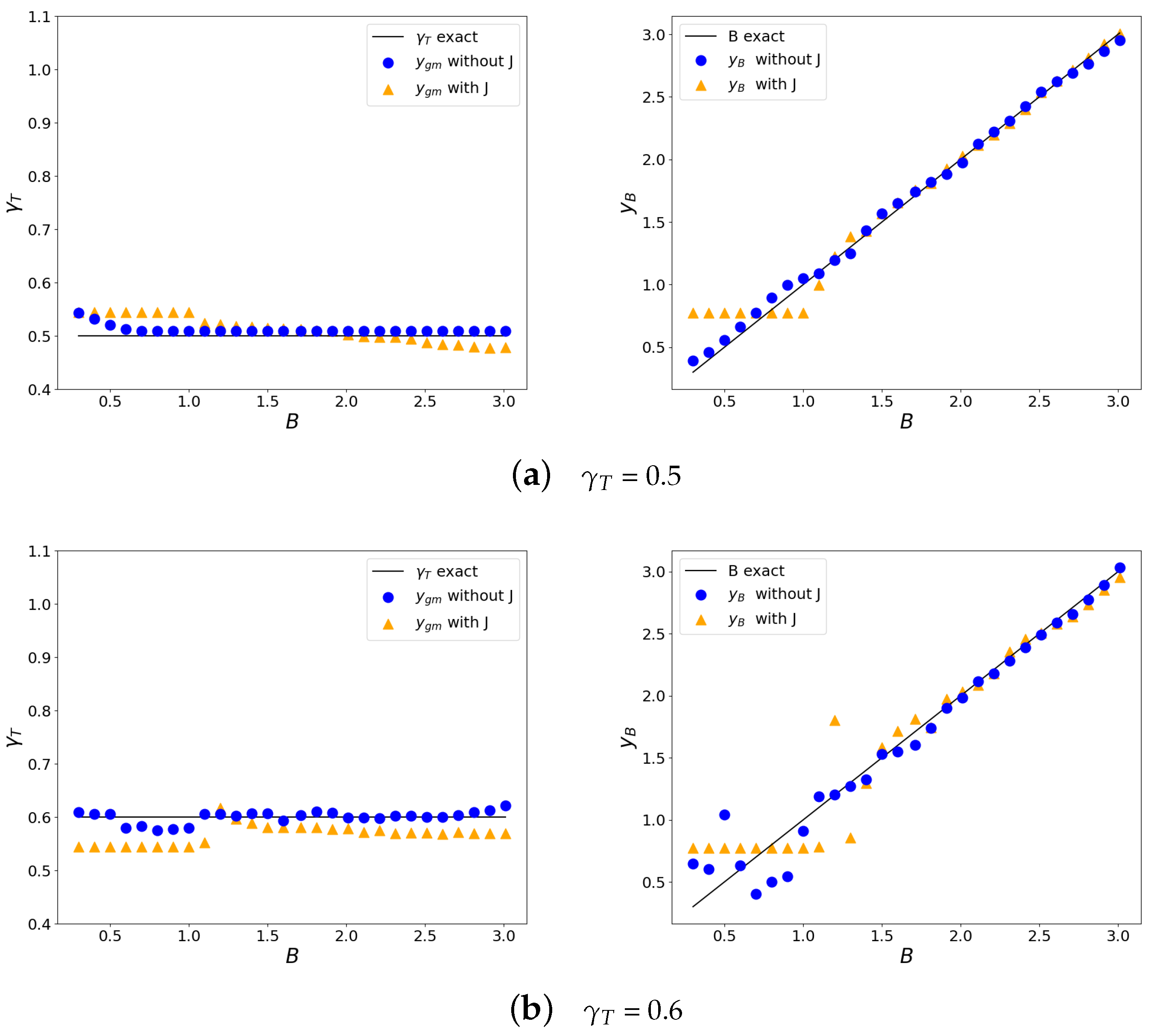
These considerations can be checked in practice with an example test. Let us consider two different throttle settings, i.e., and , that are able to generate a wide range of compressor instabilities as B varies. The accuracy of the ANN models based on the full and on the reduced datasets has been checked by testing a wide number of compressor time histories as input for the values of mentioned above. The time histories in the input are characterized by the same value of and by a different Greitzer parameter B. The results for the case with are shown in Figure 6a. The plots show the ANN-estimated values () of the parameters and B, respectively, as a function of the actual parameter B. As visible in Figure 6a (left), the prediction of is always more accurate for the ANN trained using the reduced dataset. The predicted value of the parameter B is almost the same for the two ANN models, but when , which is in the rotating stall range, the ANN trained with the reduced dataset still remains accurate, whereas the ANN trained with the full dataset freezes to an almost constant value, as shown in Figure 6a (right). Contrary to what one might expect, the information produced by seems to make the solution of the regression problem worse and the RS detection is more accurate when the evolution of the RS amplitude J is not taken into account during the ANN training. Similar considerations can be put forward for the case with , presented in Figure 6b. The same behavior is observed for a wide range of the throttle setting not reported here. Therefore, all the new ANN-trained models adopted in present work are based on the reduced set , whereas the value of J is used as an additional check of the correct detection of the instabilities.
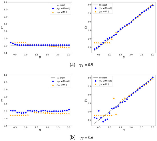
Figure 6.
Estimated () versus exact values of the Greitzer parameter B and throttle setting .
4. Results of Parameter Estimation and Instability Detection
In this section, comparisons are provided between the compressor dynamics predicted by the ANN algorithm and the original dynamics of the MG model. The two dynamics will differ by the value of the B and parameters estimated by the ANN in the former case and exact in the latter. The results obtained for the cases where the time history duration is equal to the original time interval of the trained network are discussed first. After that, the loss of accuracy related to the use of shorter time sequences in input is investigated. All time histories start from the same initial condition .
Before proceeding further, we considered the effects of the uncertainty in the evaluation of the actual Greitzer parameter B. From its definition (10), one may observe that B is affected mainly by the measure of the speed of sound, i.e., from temperature and from velocity U. This leads to the uncertainty evaluation as
Considering typical working conditions, e.g., K and m/s, we may assume that the uncertainty is of some percent of the measured value. Therefore, errors of the ANN procedure in estimating the B that fall within this uncertainty range should be considered as meaningless. Let us finally note that the uncertainty mentioned here is related to the temperature and rotational speed oscillations only. Moreover, in a practical application of this detection procedure, the accuracy and the dynamic response of the sensors used must be accounted for separately.
4.1. Results with Full Length Input Time Series
The scope of the analysis is to investigate how accurately the ANN model can extract the dynamic parameters of the system from the knowledge of a time history of a certain duration. An optimal duration of temporal window is difficult to determine anyway, since it depends on the characteristic time of the actual phenomenon occurring inside the compressor, which differs case by case.
In the present analysis, the duration of the time series in input is equal to the duration of the time series used in the ANN training phase. The nondimensional time interval is , as presented in the the four evolutions commented in Figure 3. We are therefore trying to recover the dynamics of the cases analyzed in Section 2. The parameters and are estimated by the ANN procedure and the system dynamics is reconstructed by integrating Equation (21) numerically. The actual and the estimated parameters are compared in Table 3, whereas the reconstructed and theoretical dynamics are presented in Figure 7. A brief description of the results follows.
Table 3.
Parameter detection. Full-length case. Comparison of the actual parameters () and their corresponding values () estimated by ANN.
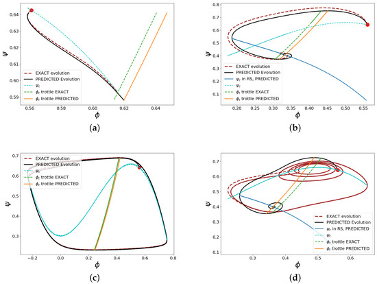
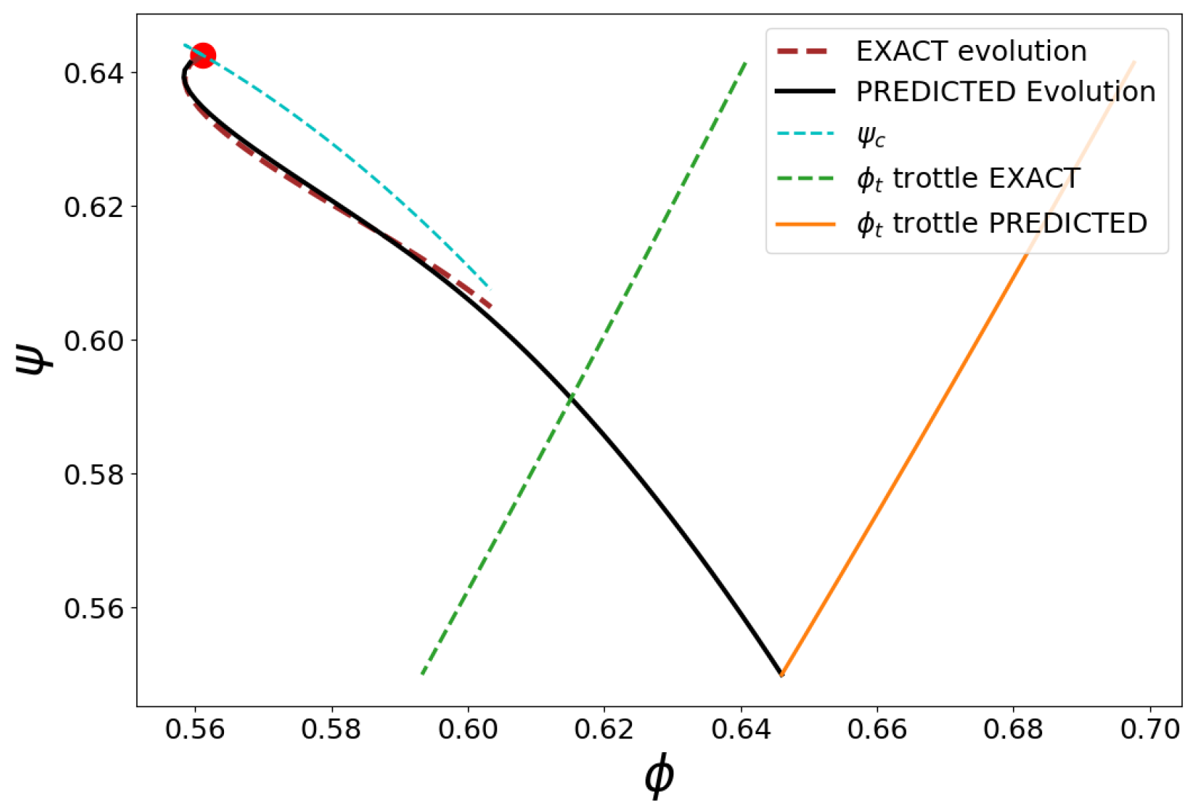
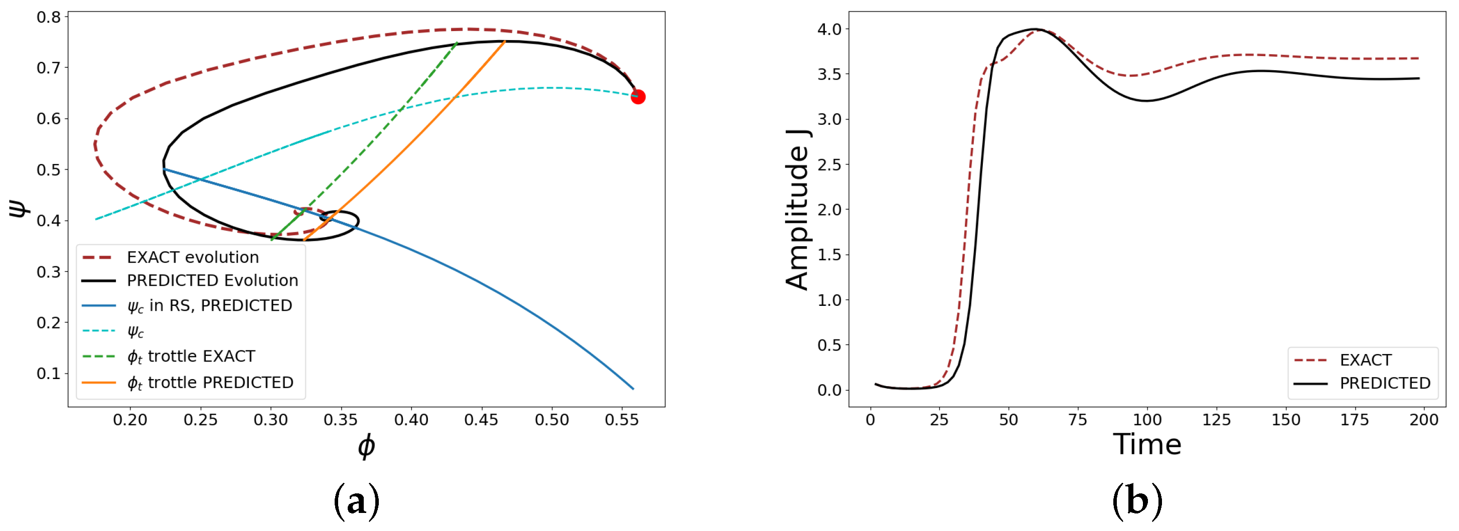
Figure 7.
Parameter estimation and reconstruction of the system dynamics. Full-length case.
Stable Point. For stable working conditions, the neural network succeeds in predicting the parameters accurately, within a relative error of 1% (Table 3). The predicted and actual dynamics are therefore in very close agreement, as shown in Figure 7a.
Rotating Stall. The RS phenomenon is well predicted by the ANN model. Although the relative error in B is around the 12% in the case presented here, the predicted system evolution still remains very close to the theoretical one (Figure 7b). The final equilibrium point at which the system works during the rotating stall is also well matched.
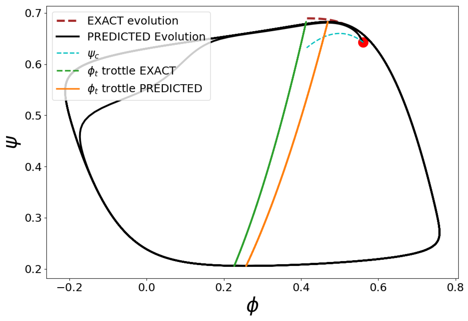
Deep Surge. The hysteresis cycle described by the values predicted by the neural network is nearly the same as the original one. Although the relative error of the predicted values of the parameters is a little bit higher than the stable point case (≤), from the plot in Figure 7c the curves of the actual and predicted evolution are almost overlapped.
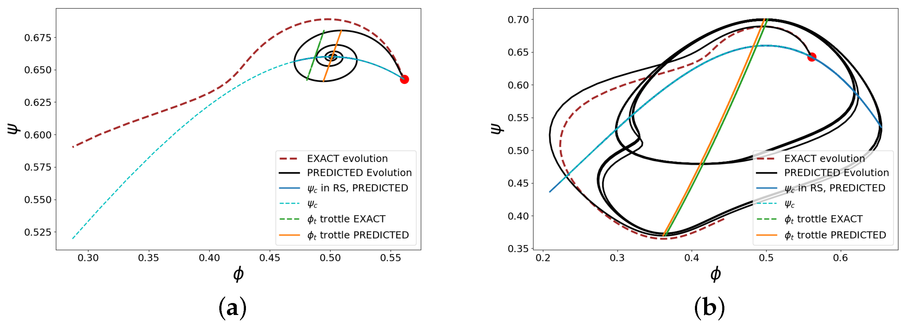
Mixed Instability. This case does not present a distinct instability, as described previously in Section 2. Observing the - plot in Figure 7d, the original system alternates RS loops with surge cycles. The system tends to RS initially, then the degradation of the compressor characteristics , due to the increasing value of J, leads the system to surge. Surging tends to decrease J and rises again. Usually, a fall in the surge is irreversible. The case we proposed is uncommon but admitted by Equation (21). It has been chosen because it is more difficult to detect. The values predicted by the ANN identify a system suffering a rotating stall (see Table 3), which in fact is the instability that comes first.
4.2. ANN Modelling with Missing Data
In the previous section, the compressor’s behavior has been observed over a period of time long enough to see the instabilities completely developed. Aiming to introduce a control that prevents the growth of instabilities, the model must manage and predict the behavior of the compressor over shorter periods of time, down to an interval shorter than the characteristic time of the instability. Now, a problem arises: the neural network is trained with input data over a fixed and longer time interval. The mismatch between the model’s expectations and the available input is one of the most challenging aspects of testing with partial data because the ANN model is designed to accept a specific input format and array shape.
The input data must be arranged in order to meet the input ANN model’s expectations, thus avoiding lower accuracy or even potential mistakes in model outputs.
Over the years, several solutions have been developed to address how to handle missing data in the ANN input [45]. A straightforward technique is zero padding, which consists of placing null values in the missing elements. It might be effective when the data can be represented as zero without introducing bias, therefore when the sequence or location of missing data has no major influence on the model’s predictions. This technique cannot be applied since zero is a value significant for our trained variables and will alter the input time history.
Imputation is another technique for estimating missing values by relying on existing ones [46]. This approach is suitable when the missing data are sparse inside the input vector so that the missing value can be replaced, for instance, by a mean or a weighted average of the nearest data points or deduced by a regression model. This is not applicable to our input time sequences since the missing data are all the elements from a certain time onwards.
Lastly, there are more complicated solutions such as Domain Knowledge or Transfer Learning [47]. The former approach requires a thorough understanding of the field to manually enter missing data, a technique that depends entirely on the programmer’s ability. Transfer learning, instead, requires the access to a pre-trained model, that accepts data with different shape size so that it can be fine-tuned to the incomplete data.
It was decided, therefore, to create several models, each one trained with different percentages of the original time interval so that each neural network would be as accurate as possible for its specific time sequence.
4.3. Results with Reduced Length Input Time Series
Three additional ANN models were trained, composed by the first 40% (), 10% () and 5% () elements of the original dataset, respectively. The time duration and the number of elements of the dataset decrease proportionally, since the series are equally spaced in time.
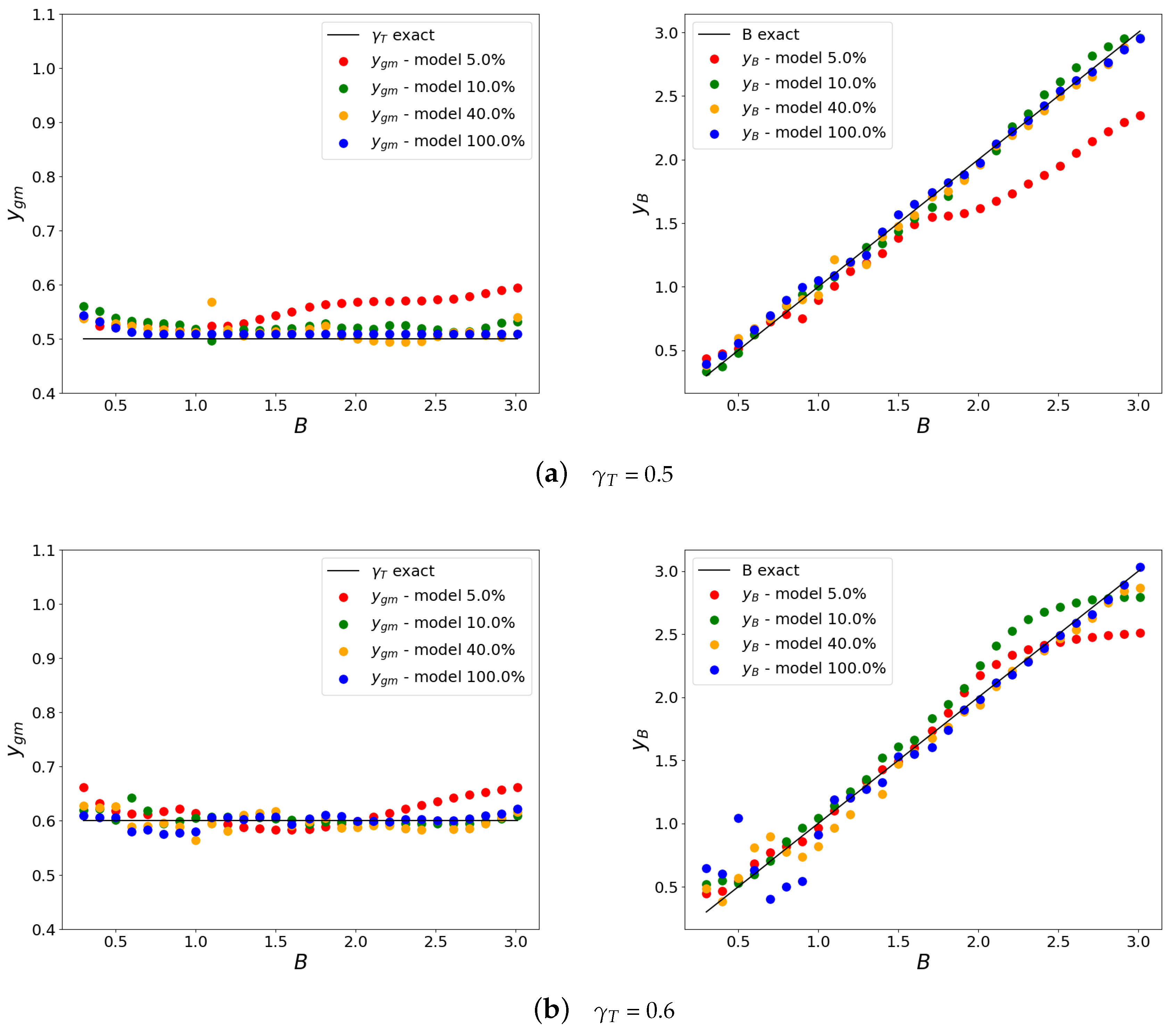
In the first step, we report the analysis for the throttle values and , as B varies, for comparison with the results obtained in Section 3. The results are presented in Figure 8 for all the datasets, including the original one (100% data). The plots show that the shorter the training time sequence is, the lower the accuracy of the predicted values for B and is. However, a few observations can be raised for the different models. Firstly, the predicted values of the throttle gain are reasonably accurate even for the model with fewer data. Moreover, in the RS range, that is for , the predicted values remain close the the correct ones (see Figure 8), thus leading to the detection of the right instability.
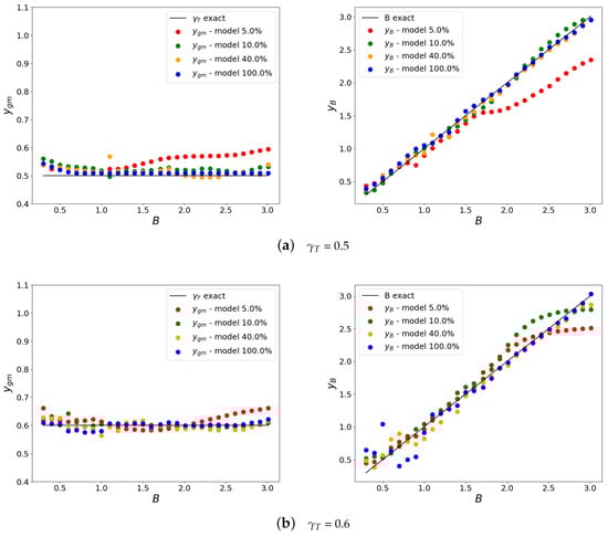
Figure 8.
Estimated () versus exact values of the Greitzer parameter B and throttle setting for input time sequences of different lengths.
The “brute force” detection of the instability by ANN is less reliable when using shorter time sequences. Anyway, by combining the available information with the knowledge of the MG model static stability, the compressor working conditions may still be identified. For instance, when from theoretical considerations [14], one may deduce the lowest value of throttle that does not lead to instability because of the change in slope of
According to the data adopted in Table 1, . Therefore, as far as the predicted value , one may exclude compressor instability without considering the estimated parameter for B.
In summary, the accuracy of the prediction of the throttle gain is the most important because it is of relevance in the identification of the instability region, whereas the prediction of B defines which kind of instability may occur. Analyzing the case for in Figure 8a, the ANN predicted value remains close to the 100% data estimation except for the shortest time sequence case (5% data), where for large B, the overestimation can even predict stable conditions. The corresponding predicted value of B (i.e., ) is well estimated in the RS range (), whereas for the 5% data case may lead to misleading the system dynamics.
Similar considerations may be put forward for the case with , although this value is very close to . The results are presented in Figure 8b. With respect to the ANN model trained by the full dataset, the 40% reduced dataset tends to underestimate , predicting a more severe instability, whereas the other two reduced models tend to predict an overestimate of and, therefore, the system stability. The detection algorithm is supposed to be applied continuously on a time moving window so that the instability can be detected in the next step.
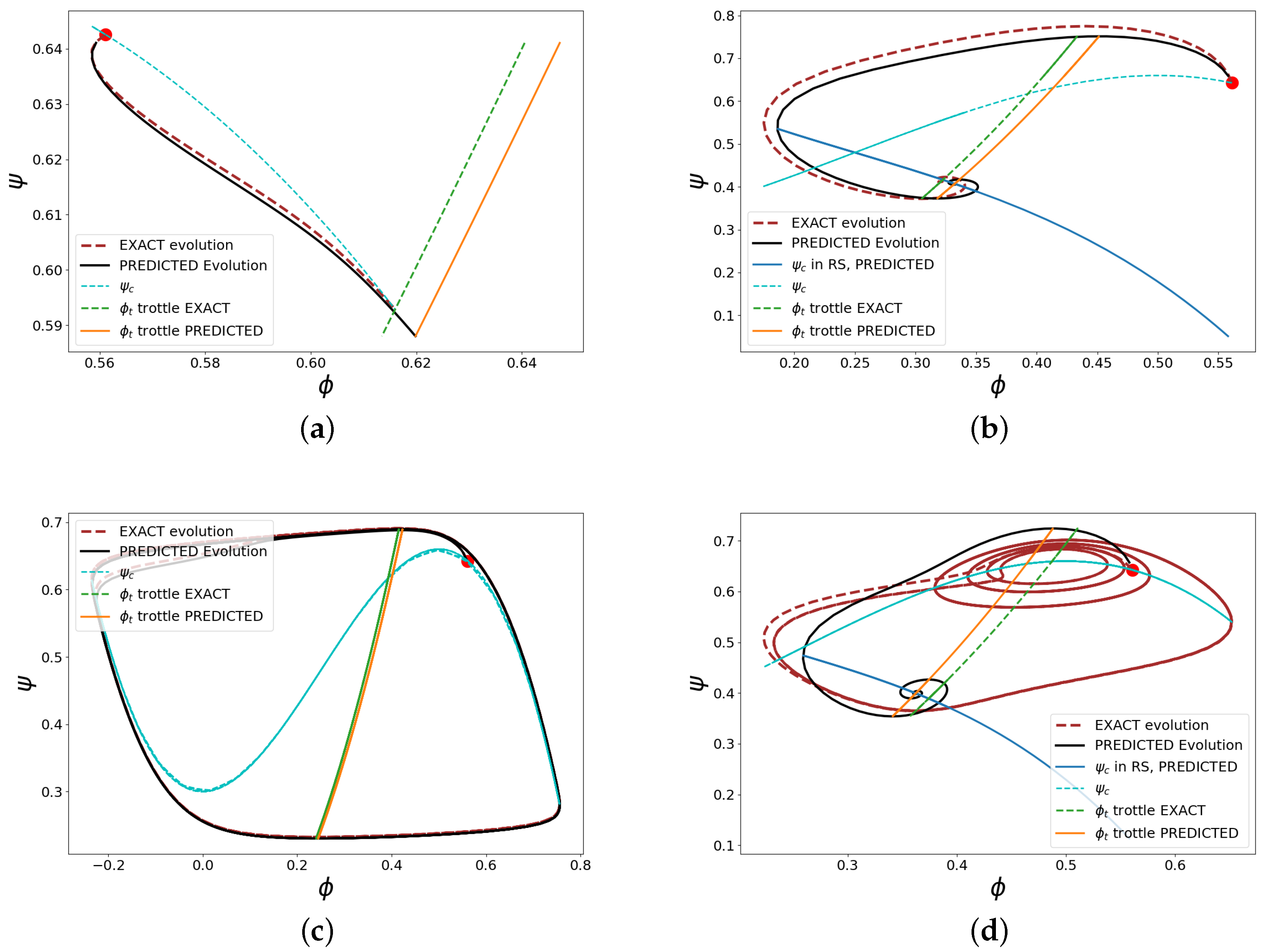
As for previous analysis, we studied the effectiveness of the algorithm in predicting the system parameters and dynamics of conditions already defined in Section 4.1.
Stable Point. The stable working condition is well captured by all the datasets. Even the shortest dataset (5% data) overpredicts by about 10% and B by 100%, as reported in Table 4. The parameter B does not affect stability and has a weak effect on the dynamics. The worst case, predicted by the 5% dataset, still maintains good agreement with the actual system dynamics within the observation window (Figure 9).
Table 4.
Stable point.
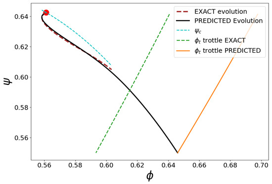
Figure 9.
Stable point prediction with 5% data.
Rotating Stall. This example of RS instability is detected by all the ANN models correctly. The highest mismatch in the prediction of is about 8% and 18% for B (see Table 5). In Figure 10, the worst case prediction of the RS dynamics is presented. Although not included in the inputs of the ANN-trained models, the evolution of the RS amplitude J can still be deduced from the detected parameters. As an example, the predicted and exact J-evolutions are compared in Figure 10b.
Table 5.
Rotating stall.
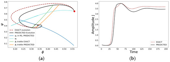
Figure 10.
RS prediction with 10% data. (a) - plane and (b) predicted RS amplitude .
Surge. Surge is well captured by all the ANN models. From Table 6, both the parameters and B are estimated within a relative error of the 6% and 3%, respectively. The DS hysteresis cycle is in good agreement with the system’s actual dynamics even for the 5% data case, as presented in Figure 11.
Table 6.
Surge.
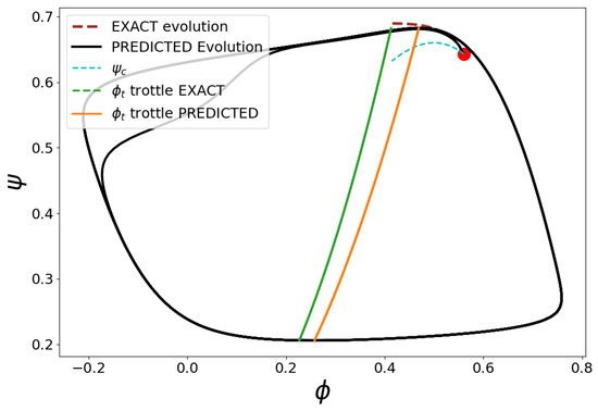
Figure 11.
Deep surge prediction with 5% data.
Mixed Instabilities. This case is the most challenging even for the ANN model based on the full dataset. The actual dynamics alternates an RS loop for several surge cycles. From Figure 3d, we may argue that the 40% dataset covers a complete evolution (), whereas the 10% and 5% dataset are trained with the part of the time series that exhibit RS only with . The predicted values of are within a 3% error and B estimations are closer to the actual values for the reduced rather than the full dataset, as visible in Table 7. Nevertheless, this accuracy does not infer the system dynamics being well captured always, because the value of is very close to the discriminant value . The ANN reduced model with 5% data estimates and therefore predicts a stable working condition (Figure 12a, whereas for the model with 10% data, the agreement is good (Figure 12b).
Table 7.
Mixed instability.
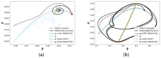
Figure 12.
Mixed instabilities with 5% (a) and 10% (b) reduced data.
4.4. Algorithm Sensitivity to the Initial Conditions and to Sensor Accuracy
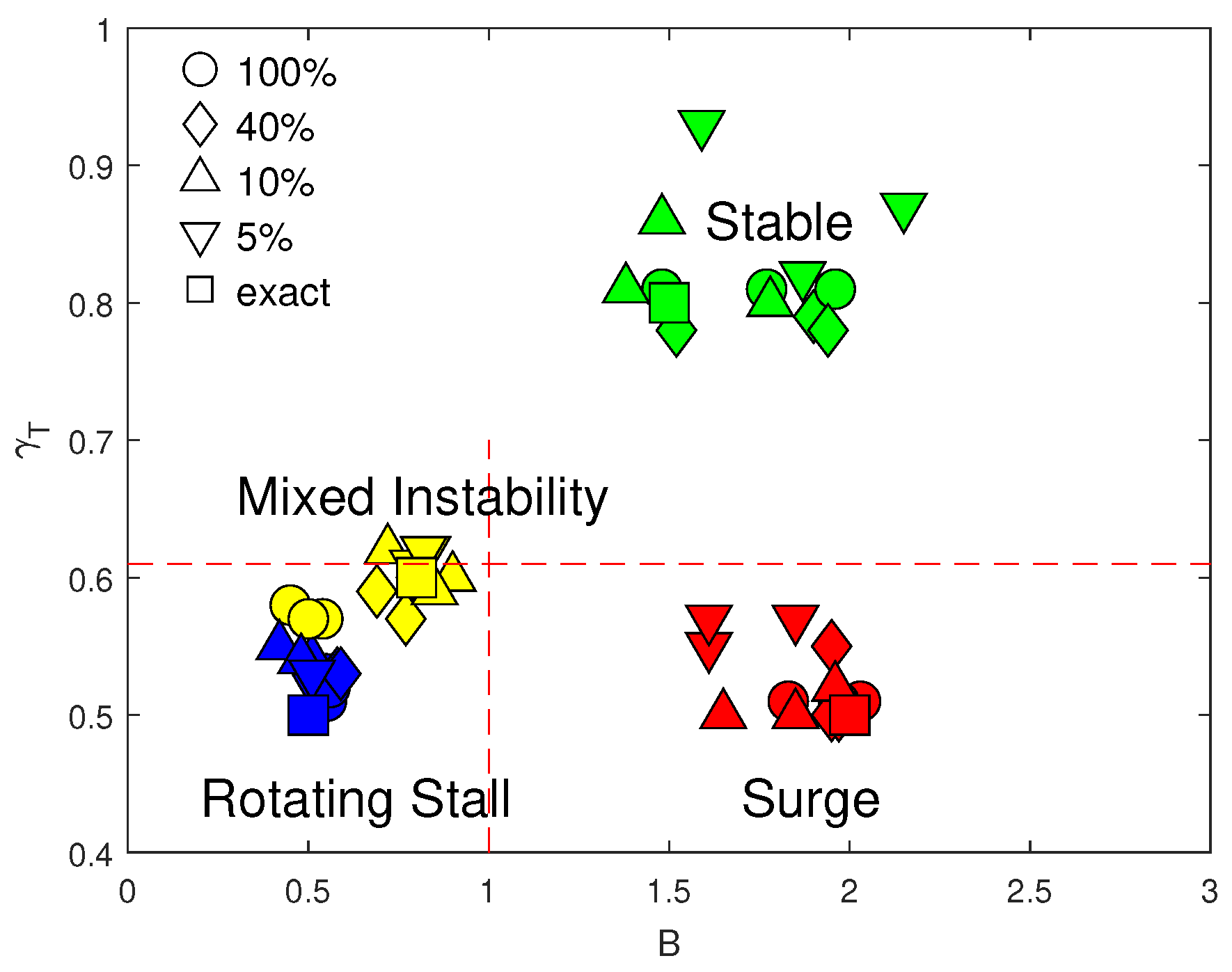
All the time sequences and examples presented in this work started from the same initial conditions . In a practical application, instead, the initial condition is a generic point in the operative range of the compressor. The plan is therefore to train the ANN model in a grid of points covering the compressor working domain and then to combine these data for approximating the compressor dynamics for starting points in between. As the simplest choice, one could use the nearest trained neighbor as initial conditions other than these grid nodes. In the present study, the analysis is limited to a couple of additional points with the opposite displacement 6% of along the compressor map, introduced to each of the four working conditions in Section 4.1 and studied by using all trained datasets of different time lengths. The results are shown in the scatter plot of Figure 13. This plot gives a synthetic view of the cluster spread because of the overall error introduced in the initial conditions and given as evidence for the ability and limitations of the reduced datasets to capture the instability correctly. Stable points are detected as stable. Working points in the stable region of the plot () are well captured and are weakly affected by the initial displacement, since the spread in B remains within that of the time sequences without displacements (). Moreover, it has already been shown in Figure 9 and Table 4 that in that region, is the most relevant parameter, and even with a 30% error in evaluating B, the system dynamics remains very close to the exact one.
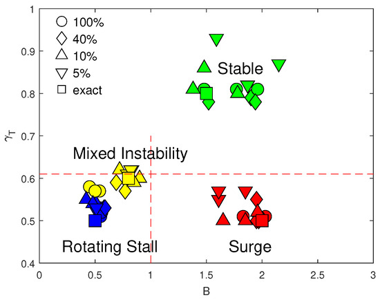
Figure 13.
Scatter plot of the estimated values for parameters B and for different (5–100%) training datasets and with uncertainty in the initial conditions. Colors define the different cases: SP (green), RS (blue), MI (yellow), and DS (red).
The same behavior can be observed when the time series in input clearly represents deep surge conditions. The error spread introduced by uncertainty remains closer to that introduced by the reduced duration ANN models. For the RS and MI cases, the spread is even lower. These cases are very close to the ideal limit between stable and unstable cases () and between RS and DS (), drawn as dashed lines in Figure 13. The overlap between the region of rotating stall, mixed instability, and classical surge is clearly visible. In these cases, the system may end up in either rotating stall or surge. Anyway, the system is monitored continuously and the evolution of the system towards the instability should be detected as the trend is more pronounced.
In a further sensitivity analysis, we studied the effect of sensor precision on the accuracy of the proposed detection algorithm. In fact, the sensors used for recording the time series are affected by measurement errors. The related uncertainty is simulated here as in [48] by introducing random displacements to all data of the clean input time series. The same ANN-trained models of the previous analyses are still used for detecting the system parameters since the clean time sequences also represent the averaged signals in the present model, as explained below.
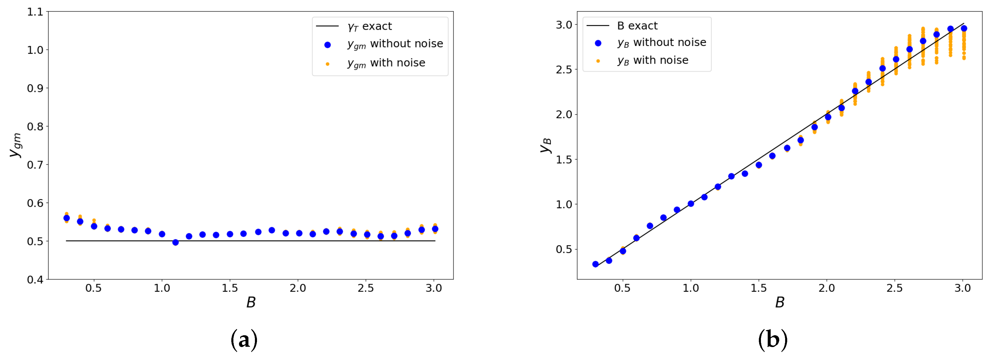
The clean time sequence in the input is perturbed by adding to each time step k random displacements . Both and follow Gaussian distributions with zero mean and standard deviations such that each measurement is affected by an error and , respectively, expressed as a percent of the measured values [48]. In the present analysis, we assumed , which is a large value. Typical values for low cost sensors are some percent of the measured value [48]. The influence of these errors is shown in Figure 14 for the case with . For each value of B, the results of the detection obtained by 50 randomly perturbed sequences have been superposed to the value obtained by the clean sequence. As visible in Figure 14a, the ANN predicted value is almost unaffected by the added noise. The predicted exhibits significant spreads for , up to the 16%, in the deep surge region. For lower B-values, the predicted is almost insensitive to the assumed sensor precision, as shown in Figure 14b.
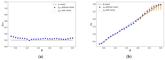
Figure 14.
Estimated (, ) versus exact values of the Greitzer parameter B and throttle setting for the 10% dataset, including sensor accuracy of 10% of the measured value, simulated by noise addition.
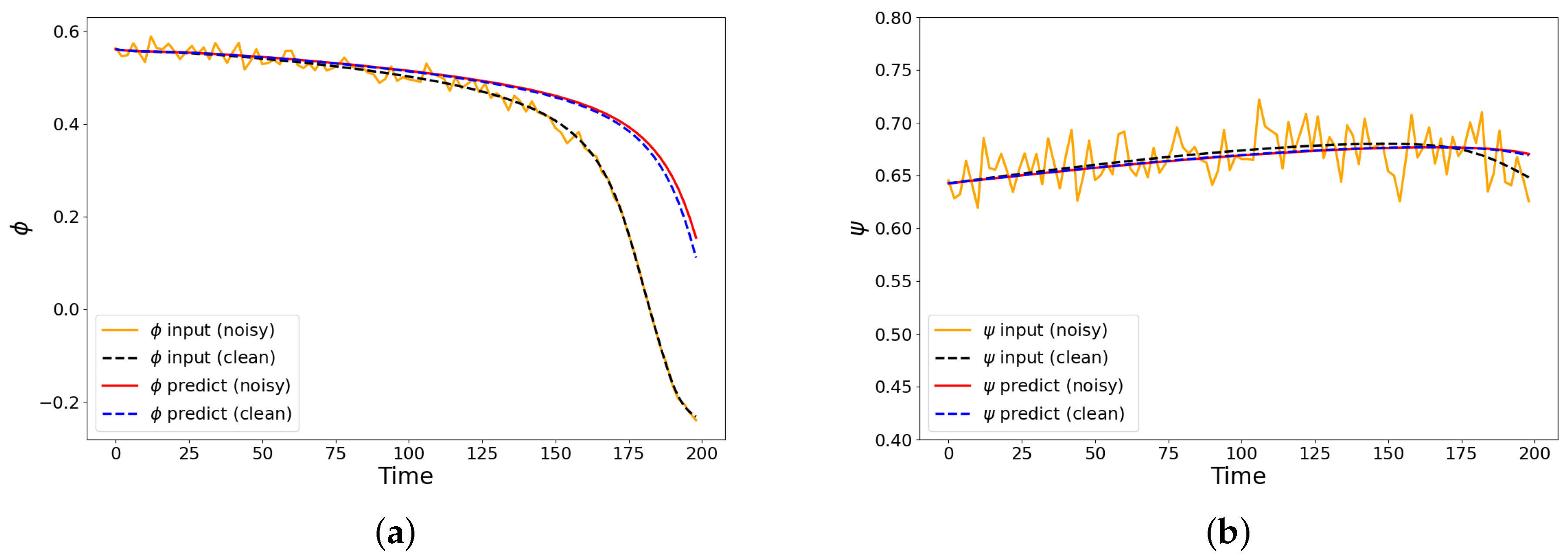
The predicted dynamics of the system is still unaffected by the added noise even in the worst case. Assuming a DS case with and B = 2.8, that is, in the wider -spread region of Figure 14b, no appreciable differences have been found between the noisy and the clean signal cases. The resulting dynamics is shown for in Figure 15a and in Figure 15b, where it can be appreciated that the two system dynamics generated by the parameters predicted by using the clean and the noisy time sequences are almost superposed.
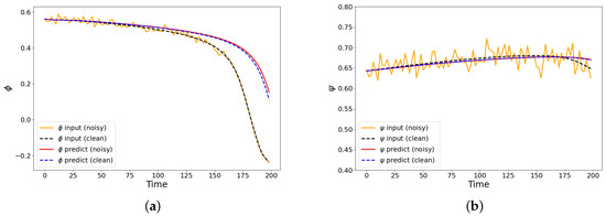
Figure 15.
Input and predicted system dynamics for case ( = 0.5; B = 2.8) with clean or noisy input time sequences. Both sensors for and measurement are supposed to have a 10% error with respect to the measured value.
5. Conclusions
The capabilities of an AI algorithm to the detect stable and unstable operating conditions of an axial compressor have been studied by using the model of the compression system model proposed by Moore and Greitzer [2,3]. It is a fluid dynamic model of general application, based on the reduction of the flow governing equations by the Galerkin method. The model allows general theoretical considerations on the instabilities of the compression system, as well as the tailoring to an actual compressor, by determining experimentally the appropriate coefficients of the manometric characteristic. The AI approach used is based on the TensorFlow platform. Providing the algorithm with a time sequence of the system evolution, we studied how to set up an AI model that recognizes the compressor operating condition and detects an eventual instability or its onset. In a practical application, the time sequence may be obtained from sensors that are monitoring the system continuously.
The study covered the entire operating field of the compressor. The results were summarized in four key situations (stable point, rotating stall, deep surge, and mixed instabilities). The effectiveness in detecting the operating condition and the related accuracy in the reconstruction of the dynamics were studied for each case, in view of an application of the AI algorithm for the design of a model-based predictive controller. It has been found that the use of a reduced set of variables, excluding the flow perturbation amplitude J, improves the algorithm accuracy.
The possibility of providing time sequences in input to the ANN model shorter than that of training was studied. Most common missing data treatment techniques have proven to be ineffective or inapplicable. We therefore studied the accuracy and effectiveness of the detection algorithm when the length of the training time series is decreased. It was found that by combining the features of the MG model and the results of the ANN detection algorithm, a time series reduced to 10% of the original training duration is still able to identify the compressor operating conditions, but in the case of mixed instability, the short term dynamics is still captured. The accuracy loss caused by the uncertainty in the initial and boundary conditions has an influence on a limited range of throttling values close to the stability value . With respect to ANN models based on the “brute force” training from the compressor recorded time sequences, the proposed approach allows for considerations both based on the theoretical model and on the reconstructed dynamics, a simpler step towards a physically-informed AI approach.
Author Contributions
Conceptualization, M.F.; methodology, M.F.; software, S.Z., D.C., and M.F.; validation, S.Z. and M.F.; formal analysis, M.F.; investigation, S.Z. and M.F.; resources, S.Z. and M.F.; data curation, S.Z., D.C., and M.F.; writing—original draft preparation, S.Z. and M.F.; writing—review and editing, S.Z., D.C., and M.F.; visualization, S.Z., D.C., and M.F.; supervision, M.F.; All authors have read and agreed to the published version of the manuscript.
Funding
This research received no external funding.
Data Availability Statement
The datasets presented in this article are not readily available because they are part of an ongoing study, further inquiries can be directed to the corresponding author.
Acknowledgments
Computational resources were provided by hpc@polito.it, a project of Academic Computing within the Department of Control and Computer Engineering at the Politecnico di Torino (http://www.hpc.polito.it).
Conflicts of Interest
The authors declare no conflicts of interest.
Abbreviations
| B | Greitzer’s parameter |
| J | first harmonic rotating stall amplitude |
| H | compressor characteristic parameter |
| equivalent compressor length | |
| intake duct length | |
| compressor exit duct length | |
| inlet total pressure | |
| plenum static pressure | |
| R | compressor wheel radius |
| U | wheel speed at mean radius |
| W | compressor characteristic parameter |
| ANN predicted value of B | |
| ANN predicted value of | |
| throttle parameter | |
| flow coefficient | |
| throttle flow characteristics | |
| nondimensional total-to static pressure rise | |
| compressor characteristics parameter | |
| compressor characteristics | |
| nondimensional time | |
| ANN | artificial neural network |
| CS | classical surge |
| DS | deep surge |
| MI | mixed instability |
| RS | rotating stall |
| SP | stable point |
References
- European Commission. Directorate-General for Mobility and Transport and Directorate-General for Research and Innovation. In Flightpath 2050—Europe’s Vision for Aviation—Maintaining Global Leadership and Serving Society’s Needs; Publications Office: Brussels, Belgium, 2011. [Google Scholar] [CrossRef]
- Moore, F.K.; Greitzer, E.M. A Theory of Post-Stall Transients in Axial Compression Systems: Part I—Development of Equations. J. Eng. Gas Turbines Power 1986, 108, 68–76. [Google Scholar] [CrossRef]
- Greitzer, E.M.; Moore, F.K. A Theory of Post-Stall Transients in Axial Compression Systems: Part II—Application. J. Eng. Gas Turbines Power 1986, 108, 231–239. [Google Scholar] [CrossRef]
- Day, I.J. Stall, Surge, and 75 Years of Research. J. Turbomach. 2015, 138, 011001. [Google Scholar] [CrossRef]
- Ferlauto, M.; Taddei, S.R. Reduced order modelling of full-span rotating stall for the flow control simulation of axial compressors. Proc. Inst. Mech. Eng. Part A J. Power Energy 2015, 229, 352–366. [Google Scholar] [CrossRef]
- Zhao, H.; Du, J.; Zhang, W.; Zhang, H.; Nie, C. A Review on Theoretical and Numerical Research of Axial Compressor Surge. J. Therm. Sci. 2022, 32, 254–263. [Google Scholar] [CrossRef]
- Fu, L.; Fu, X.; Taleb Ziabari, M. Finite-time adaptive sliding mode control for compressor surge with uncertain characteristic in the presence of disturbance. Syst. Sci. Control Eng. 2021, 9, 369–379. [Google Scholar] [CrossRef]
- Alsuwian, T.; Amin, A.A.; Iqbal, M.S.; Maqsood, M.T. A review of anti-surge control systems of compressors and advanced fault-tolerant control techniques for integration perspective. Heliyon 2023, 9, e19557. [Google Scholar] [CrossRef] [PubMed]
- Fang, Y.; Sun, D.; Xu, D.; He, C.; Sun, X. Rapid Prediction of Compressor Rotating Stall Inception Using Arnoldi Eigenvalue Algorithm. AIAA J. 2023, 61, 3566–3578. [Google Scholar] [CrossRef]
- Margalida, G.; Joseph, P.; Roussette, O.; Dazin, A. Comparison and Sensibility Analysis of Warning Parameters for Rotating Stall Detection in an Axial Compressor. Int. J. Turbomach. Propuls. Power 2020, 5, 16. [Google Scholar] [CrossRef]
- Liu, Y.; Li, J.; Du, J.; Zhang, H.; Nie, C. Reliability analysis for stall warning methods in an axial flow compressor. Aerosp. Sci. Technol. 2021, 115, 106816. [Google Scholar] [CrossRef]
- Epstein, A.H.; Williams, J.E.F.; Greitzer, E.M. Active suppression of aerodynamic instabilities in turbomachines. J. Propuls. Power 1989, 5, 204–211. [Google Scholar] [CrossRef]
- Billoud, G.; Galland, M.A.; Huu, C.H.; Candel, S. Adaptive Active Control of Instabilities. J. Intell. Mater. Syst. Struct. 1991, 2, 457–471. [Google Scholar] [CrossRef]
- Gravdahl, J.T.; Egeland, O. Close Coupled Valve Control of Surge and Rotating Stall for the Moore-Greitzer Model. In Advances in Industrial Control; Springer: London, UK, 1999; pp. 63–107. [Google Scholar] [CrossRef]
- Elcrat, A.; Ferlauto, M.; Zannetti, L. Point vortex model for asymmetric inviscid wakes past bluff bodies. Fluid Dyn. Res. 2014, 46, 031407. [Google Scholar] [CrossRef]
- de Jager, B. Rotating stall and surge control: A survey. In Proceedings of the 1995 34th IEEE Conference on Decision and Control, New Orleans, LA, USA, 13–15 December 1995; p. CDC-95. [Google Scholar] [CrossRef]
- Sheng, H.; Chen, Q.; Li, J.; Li, Z.; Wang, Z.; Zhang, T. Robust adaptive backstepping active control of compressor surge based on wavelet neural network. Aerosp. Sci. Technol. 2020, 106, 106139. [Google Scholar] [CrossRef]
- Liaw, D.C.; Abed, E.H. Active control of compressor stall inception: A bifurcation-theoretic approach. Automatica 1996, 32, 109–115. [Google Scholar] [CrossRef]
- Backi, C.J.; Gravdahl, J.T.; Skogestad, S. Robust control of a two-state Greitzer compressor model by state-feedback linearization. In Proceedings of the 2016 IEEE Conference on Control Applications (CCA), Buenos Aires, Argentina, 19–22 September 2016. [Google Scholar] [CrossRef]
- Neverlien, A.; Moe, S.; Gravdahl, J.T. Compressor Surge Control Using Lyapunov Neural Networks. Model. Identif. Control. A Nor. Res. Bull. 2020, 41, 41–49. [Google Scholar] [CrossRef]
- Shehata, R.S.; Abdullah, H.A.; Areed, F.F.G. Fuzzy logic surge control in constant speed centrifugal compressors. In Proceedings of the 2008 Canadian Conference on Electrical and Computer Engineering, IEEE, Niagara Falls, ON, Canada, 4–7 May 2008. [Google Scholar] [CrossRef]
- Divya, N.; Narayanappa, C.; Gangadhariah, S.; Prasad, V. Design and Performance Analysis of Anti-Surge Control Mechanism for Compressor System using Neural Networks. Int. J. Adv. Comput. Sci. Appl. 2022, 13, 710–718. [Google Scholar] [CrossRef]
- Antão, R.; Antunes, J.; Mota, A.; Escadas Martins, R. Model Predictive Control of Non-Linear Systems Using Tensor Flow-Based Models. Appl. Sci. 2020, 10, 3958. [Google Scholar] [CrossRef]
- Ferlauto, M.; Marsilio, R. A computational approach to the simulation of controlled flows by synthetic jets actuators. Adv. Aircr. Spacecr. Sci. 2014, 2, 77–94. [Google Scholar] [CrossRef]
- Kadivar, A.; Amanifard, N.; Deylami, H.M.; Dolati, F. Flow separation control in an axial compressor cascade using various arrangement of plasma actuator. J. Electrost. 2021, 112, 103580. [Google Scholar] [CrossRef]
- Willems, F.; Heemels, W.; de Jager, B.; Stoorvogel, A.A. Positive feedback stabilization of centrifugal compressor surge. Automatica 2002, 38, 311–318. [Google Scholar] [CrossRef]
- Tucci, L. Analysis and Simulation of Instabilities in Axial Compressors: Engine Model Integration. Master’s Thesis, Aerospace Engineering, Politecnico di Torino, Turin, Italy, 2022. [Google Scholar]
- Mansoux, C.; Gysling, D.; Setiawan, J.; Paduano, J. Distributed nonlinear modeling and stability analysis of axial compressor stall and surge. In Proceedings of the 1994 IEEE American Control Conference—ACC ’94, Baltimore, MD, USA, 29 June–1 July 1994. [Google Scholar] [CrossRef]
- Li, J.; Teng, J.; Ferlauto, M.; Zhu, M.; Qiang, X. An improved stall prediction model for axial compressor stage based on diffuser analogy. Aerosp. Sci. Technol. 2022, 127, 107692. [Google Scholar] [CrossRef]
- Ferlauto, M.; Marsilio, R. Numerical Simulation of the Unsteady Flowfield in Complete Propulsion Systems. Adv. Aircr. Spacecr. Sci. 2018, 5, 349–362. [Google Scholar] [CrossRef]
- Gu, G.; Sparks, A.; Banda, S. An overview of rotating stall and surge control for axial flow compressors. IEEE Trans. Control Syst. Technol. 1999, 7, 639–647. [Google Scholar] [CrossRef]
- Xu, D.; He, C.; Sun, D.; Sun, X. Stall inception prediction of axial compressors with radial inlet distortions. Aerosp. Sci. Technol. 2021, 109, 106433. [Google Scholar] [CrossRef]
- Xu, D.; Dong, X.; Zhou, C.; Sun, D.; Gui, X.; Sun, X. Effect of rotor axial blade loading distribution on compressor stability. Aerosp. Sci. Technol. 2021, 119, 107230. [Google Scholar] [CrossRef]
- Abadi, M.; Agarwal, A.; Barham, P.; Brevdo, E.; Chen, Z.; Citro, C.; Corrado, G.S.; Davis, A.; Dean, J.; Devin, M.; et al. TensorFlow: Large-Scale Machine Learning on Heterogeneous Distributed Systems. arXiv 2016, arXiv:1603.04467. [Google Scholar] [CrossRef]
- Pang, B.; Nijkamp, E.; Wu, Y.N. Deep Learning With TensorFlow: A Review. J. Educ. Behav. Stat. 2019, 45, 227–248. [Google Scholar] [CrossRef]
- Gao, Z.; Cecati, C.; Ding, S.X. A Survey of Fault Diagnosis and Fault-Tolerant Techniques—Part I: Fault Diagnosis With Model-Based and Signal-Based Approaches. IEEE Trans. Ind. Electron. 2015, 62, 3757–3767. [Google Scholar] [CrossRef]
- Park, P.; Marco, P.D.; Shin, H.; Bang, J. Fault Detection and Diagnosis Using Combined Autoencoder and Long Short-Term Memory Network. Sensors 2019, 19, 4612. [Google Scholar] [CrossRef]
- Sztyber, A.; Chechlinski, L.; Syfert, M.; Wnuk, P.; Lipnicki, P.; Lewandowski, D. Analysis of Applicability of Deep Learning Methods in Compressor Fault Diagnosis. In Proceedings of the Workshop on Principles of Diagnosis 2018, Warsaw, Poland, 27–30 August 2018. [Google Scholar]
- Pakatchian, M.R.; Ziamolki, A.; Alhuyi Nazari, M. Applications of machine learning approaches in aerodynamic aspects of axial flow compressors: A review. Front. Energy Res. 2023, 11, 1135055. [Google Scholar] [CrossRef]
- Hipple, S.M.; Bonilla-Alvarado, H.; Pezzini, P.; Shadle, L.; Bryden, K.M. Using Machine Learning Tools to Predict Compressor Stall. J. Energy Resour. Technol. 2020, 142, 070915. [Google Scholar] [CrossRef]
- Chollet, F. Keras. GitHub. 2015. Available online: https://www.scirp.org/reference/ReferencesPapers?ReferenceID=1887532 (accessed on 2 April 2024).
- Staats, K.; Pantridge, E.; Cavaglia, M.; Milovanov, I.; Aniyan, A. TensorFlow enabled genetic programming. In Proceedings of the GECCO ’17 Genetic and Evolutionary Computation Conference Companion, ACM, Berlin, Germany, 15–19 July 2017. [Google Scholar] [CrossRef]
- Bisong, E. Building Machine Learning and Deep Learning Models on Google Cloud Platform: A Comprehensive Guide for Beginners; Apress: New York, NY, USA, 2019. [Google Scholar] [CrossRef]
- Pedregosa, F.; Varoquaux, G.; Gramfort, A.; Michel, V.; Thirion, B.; Grisel, O.; Blondel, M.; Müller, A.; Nothman, J.; Louppe, G.; et al. Scikit-learn: Machine Learning in Python. arXiv 2012, arXiv:1201.0490. [Google Scholar] [CrossRef]
- Little, R.; Rubin, D. Statistical Analysis with Missing Data, 3rd ed.; Wiley: Hoboken, NJ, USA, 2019. [Google Scholar] [CrossRef]
- Spinelli, I.; Scardapane, S.; Uncini, A. Missing data imputation with adversarially-trained graph convolutional networks. Neural Netw. 2020, 129, 249–260. [Google Scholar] [CrossRef]
- Khan, H.; Wang, X.; Liu, H. Handling missing data through deep convolutional neural network. Inf. Sci. 2022, 595, 278–293. [Google Scholar] [CrossRef]
- Resta, E.; Ferlauto, M.; Marsilio, R. AI assisted detection of shock motions inside a transonic duct. In Proceedings of the International Conference on Computational Intelligence And Computing Applications-21 (ICCICA-21), Nagpur, India, 18–19 June 2021; AIP Publishing: Melvill, NY, USA, 2022. [Google Scholar] [CrossRef]


Disclaimer/Publisher’s Note: The statements, opinions and data contained in all publications are solely those of the individual author(s) and contributor(s) and not of MDPI and/or the editor(s). MDPI and/or the editor(s) disclaim responsibility for any injury to people or property resulting from any ideas, methods, instructions or products referred to in the content. |
© 2024 by the authors. Licensee MDPI, Basel, Switzerland. This article is an open access article distributed under the terms and conditions of the Creative Commons Attribution (CC BY) license (https://creativecommons.org/licenses/by/4.0/).